Storm-Time Features of the Ionospheric ELF/VLF Waves and Energetic Electron Fluxes Revealed by the China Seismo-Electromagnetic Satellite

Abstract

This study reports the temporal and spatial distributions of the extremely/very low frequency (ELF/VLF) wave activities and the energetic electron fluxes in the ionosphere during an intense storm (geomagnetic activity index Dst of approximately −174 nT) that occurred on 26 August 2018, based on the observations by a set of detectors onboard the China Seismo-Electromagnetic Satellite (CSES). A good correlation of the ionospheric ELF/VLF wave activities with energetic electron precipitations during the various storm evolution phases was revealed. The strongest ELF/VLF emissions at a broad frequency band extending up to 20 kHz occurred from the near-end main phase to the early recovery phase of the storm, while the wave activities mainly appeared at the frequency range below 6 kHz during other phases. Variations in the precipitating fluxes were also spotted in correspondence with changing geomagnetic activity, with the max values primarily appearing outside of the plasmapause during active conditions. The energetic electrons at energies below 1.5 MeV got strong enhancements during the whole storm time on both the day and night side. Examinations of the half-orbit data showed that under the quiet condition, the CSES was able to depict the outer/inner radiation belt as well as the slot region well, whereas under disturbed conditions, such regions became less sharply defined. The regions poleward from geomagnetic latitudes over 50° were found to host the most robust electron precipitation regardless of the quiet or active conditions, and in the equatorward regions below 30°, flux enhancements were mainly observed during storm time and only occasionally in quiet time. The nightside ionosphere also showed remarkable temporal variability along with the storm evolution process but with relatively weaker wave activities and similar level of fluxes enhancement compared to the ones in the dayside ionosphere. The ELF/VLF whistler-mode waves recorded by the CSES mainly included structure-less VLF waves, structured VLF quasi-periodic emissions, and structure-less ELF hiss waves. A wave vector analysis showed that during storm time, these ELF/VLF whistler-mode waves obliquely propagated, mostly likely from the radiation belt toward the Earth direction. We suggest that energetic electrons in the high latitude ionosphere are most likely transported from the outer radiation belt as a consequence of their interactions with ELF/VLF waves.

1. Introduction

Within the solar-terrestrial system, the ionospheric layers can mirror both Earthward and Sunward disturbances at various scales. From the Earth direction, namely from the lithosphere or atmosphere, the disturbances include the relatively weak but detectable seismic precursor anomalies [1], the strong radio waves emitted by powerful ground-based very low frequency (VLF) transmitters [2], the harmonic radiation from the electric power lines [3], and the strong whistler-mode waves induced by lightning/thunderstorms in the atmosphere. From the Sun direction, the disturbances coming from above the ionosphere are mainly related to the Sun, which releases coronal mass ejections (CMEs) and solar flares, as well as the resultant geomagnetic storm/substorm activity. In particular, there is a magnetic field-line mapping of the magnetosphere onto the high-latitude ionosphere, along which field-line currents, possibly associated with magnetospheric polarization fronts, enter the post-midnight ionosphere and leave it from the pre-midnight side, thus feeding the strong aurora electrojet [4,5]. This makes the ionosphere a highly dynamic system where a variety of intense electromagnetic emissions and energetic particle precipitations are detected due to multiple layer interactions with the lithosphere, atmosphere, and magnetosphere, as well as solar wind [4,5,6,7,8].

The electromagnetic emissions excited in the extremely/very low frequency (ELF/VLF) range [9,10,11,12,13] are the most direct outcomes of this dynamic system. The most commonly observed typical electromagnetic waves at ELF/VLF bands are the whistler-mode waves [9,14,15,16,17,18], which include the whistler-mode VLF chorus [12,16,19], quasi-periodic waves [13,15,20], ELF hiss [21,22,23], and strong whistlers induced by lightning, VLF radio wave transmitters, or other sources [22,24]. These typical whistler-mode waves play significant roles either in the acceleration or loss process of relativistic electrons in the Earth’s outer radiation belt [14,17,25]. The VLF chorus mainly appears at frequency from 0.1 to 0.8 f_ce (the equatorial electron cyclotron frequency) and can efficiently accelerate relativistic electrons (E > MeV) [14]. Zhima et al. [10] firstly found the evidence of whistler-mode chorus penetrating the plasmapause and entering into the low altitude ionosphere, and Zhang et al. [26] firstly reported that chorus waves in the magnetosphere accelerated energetic electrons (1–3 MeV) in the ionosphere from the China Seismo-Electromagnetic Satellite (CSES) observations. ELF hiss waves are structure-less and incoherent electromagnetic waves that preferentially appear at a broad frequency range from several hundred Hz to 3 kHz, playing vital roles in either the loss of energetic electrons or the formation of radiation belt slot region [22,27,28]. Another important ELF/VLF whistler-mode wave often appearing in the ionosphere is the quasi-periodic (QP) wave at frequencies from several hundred Hz to ~4 kHz with varying periodic modulations of wave intensity over time scales from several seconds to a few minutes; they are often observed by low Earth orbit (LEO) satellites and ground stations [13,15]. Zhima et al. [20] reported the well-pronounced rising-tone structure QP waves and simultaneous energetic electron precipitations (from ~400 keV to 1 MeV) in the high-latitude ionosphere firstly based on the CSES’s observations.

Because they are simultaneously observed with the strong ELF/VLF wave activity, changes in the fluxes of energetic particle populations are usually checked for. In the context of radiation-belt dynamics, it is widely accepted that ELF/VLF whistler-mode waves represent the main candidate for the acceleration/loss of particles during storm time [17,29], so they have been given increasing attention due to their impact on the dynamics of near-Earth space. Benck et al. [18] revealed the global distribution of ionospheric ELF/VLF wave intensities and energetic electron precipitations during an intense magnetic storm by making use of DEMETER (Detection of Electromagnetic Emissions Transmitted from Earthquake Regions) observations (altitude: ~710 km in 2004), and a good correlation between waves and particle precipitations at different stages of storm evolution was revealed. Still relying on DEMETER observations, Zhima et al. [9] statistically analyzed the temporal–spatial variations of the ionospheric ELF/VLF waves during all the intense CME-driven storms that occurred from 2005 to 2009 (altitude: ~660 km), specifically showing how the ELF/VLF waves in different frequency ranges were excited across the L shell space during the evolution of this type of storms.

Since the successful operation of the French DEMETER satellite (2005–2010), which was mainly dedicated to the investigation of ionospheric disturbances possibly associated with the strong earthquakes, volcanoes, or anthropogenic activities from the lithosphere [30], a growing number of studies [8,11,31,32] obtained from DEMETER observations have been suggesting that satellites probing electromagnetism in LEO space can be regarded as promising tools to monitor natural hazards [33].

However, since DEMETER was decommissioned in December 2010, there lacks similar type of electromagnetic satellite in the ionosphere to provide first-hand observations for studying natural disasters until the recent successful launch of the CSES on 2 February 2018 at an altitude of 507 km in the ionosphere [33,34]. The CSES is part of China’s Zhangheng mission, which is aimed to launch both electromagnetic and gravity satellites in near-Earth orbit within the next few decades. The Zhangheng mission is named after the ancient scientist Zhangheng who invented the world’s first seismoscope in the second century CE. The Zhangheng-01 (ZH-1) mission is dedicated to the electromagnetic satellites with three planned consecutive launches—it is also known as the CSES; Zhangheng-02, in the preparation phase at present, is dedicated to gravity satellites.

The first probe of the CSES mission was successfully launched into a sun-synchronous circular orbit. The second probe will be launched into the same orbit before December 2022, but it will operate at the opposite side of the Earth, which means that two probes will be operating on both the day and night sides of the ionosphere by 2023 (the first probe was designed to span a five-year lifetime but is expected to operate longer).

Since its successful launch in 2018, the CSES has been providing valuable measurements about the electromagnetic field across a broad frequency range from ultra-low frequency (ULF) to very low frequency (VLF), and even to the high frequency (HF) of the electric field, as well as fluxes of energetic electrons at energies from 0.1 to 50 MeV. In view of the importance of electromagnetic wave activities and energetic electron populations for natural hazard science, the purpose of this paper was to investigate the features of waves and particles in LEO space by using CSES observations. Based on previous DEMETER studies [9,18] (at altitudes from ~660 to 710 km), this work presents CSES data to describe the temporal and spatial distribution of the ionospheric ELF/VLF waves and energetic particle fluxes during the G3-class storm (Dst minimum of −174 nT) that occurred on 26 August 2018. A brief introduction to the CSES and associated payloads is provided in Section 2, while the distributions of ionospheric ELF/VLF waves and energetic electron fluxes are presented in Section 3. Section 4 offers a discussion concerning experimental observations, and Section 5 briefly summarizes the main results.

2. Satellite and Data

The main scientific objective of the CSES is to monitor ionospheric perturbations associated with natural hazards (mainly with strong earthquakes) in the quest for possible earthquake forecasting. To serve the need of emergence response to disastrous earthquakes, such as the 2008 Mw 7.9 Wenchuan earthquake, the CSES was designed to provide real-time data over China’s territory via a direct downlink to the ground segment.

The CSES completes 15.2 orbits around Earth per day, with an orbital period of ~94.6 min and a five-day recursive period over the same geographic area with the ascending/descending node local time of 02 a.m./02 p.m., respectively. Its payloads allow for the measurement of the electromagnetic field, energetic particles, and in-situ and profile ionosphere parameters. The diverse physical parameters obtained by the CSES can support the comprehensive research of geo-/space physics and radio science.

The payloads involved in this study are briefly introduced here. The background geomagnetic field is measured by a high precision magnetometer (HPM) [35], which includes two fluxgate sensors [36] and a coupled dark-state magnetometer [37], providing both vector and scalar values of the total geomagnetic field in a frequency range from DC to 15 Hz and a sampling rate of 1 Hz for the scalar geomagnetic field detection. The variant magnetic field from 10 Hz to 20 kHz is measured by a tri-axis search-coil magnetometer (SCM) mounted on the end part of a 4.5-m-long boom to avoid the artificial electromagnetic interferences induced by the satellite platform itself [38,39]. The SCM provides data in the three frequencies bands of ULF (10 to 200 Hz), ELF (from 200 Hz to 2.2 kHz), and VLF (1.8 to 20 kHz) with sampling rates of 1024 Hz, 10.24 kHz, and 51.2 kHz, respectively. The electric field is detected by an electric field detector (EFD), which consists of four spherical sensors mounted at the near-end part of four booms (4.5 m long) [40], measuring the electric field in four frequency channels: ULF (DC to16 Hz), ELF (from 6 Hz to 2.2 kHz), VLF (1.8 to 20 kHz), and HF (from 18 kHz to 3.5 MHz), with sampling rates of 128 Hz, 5 kHz, 50 kHz, and 10 MHz, respectively. The energetic particles are recorded by the high energetic particle package (HEPP), with three sub-detectors (HEPP-H, HEPP-L, and HEPP-X) providing the energy spectrum and pitch-angle distribution of charged particles (protons: from 2 MeV to 200 MeV; electrons: from 100 keV to 50 MeV) and soft X-ray emission from solar events [41,42]. In this study, HEPP-L was selected to measure electron fluxes at energies from 0.1 to 3 MeV and corresponding pitch-angle distributions. HEPP-L contains nine silicon-slice units and one anti-coincidence detector with an angular resolution of 5° and a maximum field-view of 100° × 30° [42].

3. Observations

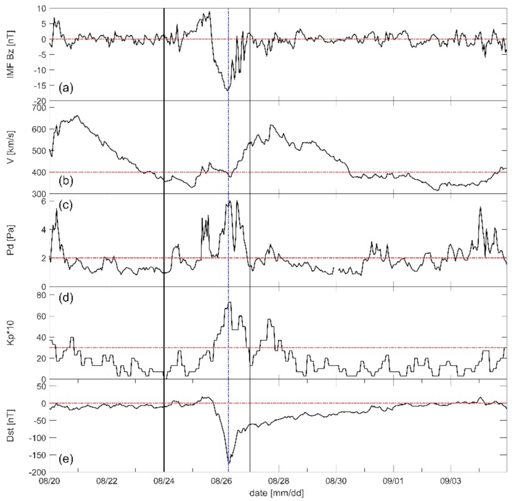
Figure 1 shows major parameters describing the solar wind conditions and the geomagnetic activity indices Dst and Kp from 20 August to 4 September 2018. It can be seen that the north–south component of the interplanetary magnetic field (IMF Bz) in the GSM (geocentric solar magnetospheric) coordinate system suffered a slight northern enhancement of up to ~9 nT at ~14:00 UT on 25 August 2018 before suddenly turning southward with a steep drop to the minimum value of −16.8 nT at 05:00 UT on 26 August, followed by a very fluctuating recovery back to an average value of ~0 nT. This prolonged southward alignment of the IMF Bz triggered a dayside magnetic field line reconnection at the magnetopause, directly inducing a strong geomagnetic storm during which the geomagnetic equatorial Dst index dropped to the minimum value of −174 nT at 06:00 to 07:00 UT on 26 August, followed by a long-term recovery phase lasting until 3 September 2018. The source for this intense geomagnetic storm was identified as the interplanetary coronal mass ejection (ICME) from the Sun that occurred downstream of a filament eruption on 20 August 2018 [43]. In particular, from the point of view of solar wind velocity, this ICME event was pretty interesting, since a fast speed of more than 600 km/s, along with the subsequent consistent slowdown to less than 400 km/s and slight recovery, was reached prior to the onset of the geomagnetic storm before again giving rise to a fast speed (up to ~500 km/s) in the early recovery phase and a new marked decrease in the late part of the recovery. The solar wind dynamic pressure, which was a direct indicator of solar wind and ion and electron density, intensely increased during the main and early recovery phases, reached the peak at the early recovery phase, and remained fluctuating around 2 nPa for the most of other times.

The effects of this geomagnetic storm on Earth’s ionosphere were investigated by Younas et al. [44] based on multi-parameter measurements, including total electron content (TEC), geomagnetic field intensity, and O/N2 ratio data, and theit results showed that a positive ionosphere storm (increase of TEC) in the southern hemisphere and a negative storm in the northern one were formed. Yang et al. [5] also reported simultaneous responses from multi-type CSES payloads to this event, thus leading to the assessment of the good performance of the CSES in reacting to the different phases of the storm. Strong ELF/VLF emissions were especially observed, with the simultaneous enhancement of energetic electron fluxes in the South Atlantic Anomaly (SAA), outer/inner radiation belt, and slot region [5].

In the following section, we mainly focus on the temporal and spatial distributions of the storm-time ELF/VLF waves across a broad frequency band from 200 Hz to 20 kHz, as well as the energetic electron fluxes at energies 0.1 MeV < E < 3.0 MeV by using data from the SCM, EFD, and HEPP-L onboard the CSES.

We adopted the superposed epoch analysis method by defining the reference time t₀ as the time of Dst minimum (from 06:00 UT on 26 August 2018), as we did in previous work [6]. We mainly computed the average power spectral density (PSD) values of the electric and magnetic field at a frequency range of 1 kHz < f < 2 kHz, as well as the average energetic electron fluxes data at an energy level of 1 MeV < E < 3 MeV for each orbit. Then, these data were binned as a function of L shell in steps of 0.2 L, with a time interval of 1 h in the epoch time period from t₀ − 30 h to t₀ + 90 h (namely, from 00: 00 UT 25 August to 00:00 UT 30 August).

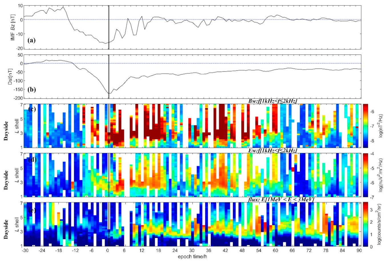
The results are presented in Figure 2 (dayside) and Figure 3 (nightside). As seen in Figure 2c,d, before the storm initial phase that began at epoch time t₀ − 16 h (14:00 UT on 25 August 2018) and indicated by a slight increase of Dst index, the ionosphere remained in a relatively quiet electromagnetic environment (denoted by the blue areas in Figure 2c,d from epoch time t = −30 h to −16 h). Meanwhile, along with the consistent southern reversal of IMF Bz and the corresponding decrease of the Dst index, the wave activities started to grow up (~t = −9 h) and reached ELF/VLF maximum emissions around the end of the main phase and the beginning of the recovery phase (t = −2 to 20 h). We can see a close correlation between the ELF/VLF wave activities, the IMF Bz, and the solar wind (velocity and pressure); when IMF Bz and solar wind were stable at times when IMF Bz was close to 0 nT, the wave activities were weak (e.g., 20 h < t < 28 h and 60 h < t < 72 h), while when the solar wind conditions were strongly fluctuating, strong ELF/VLF emissions were observed (e.g., 2 h < t < 20 h).

Figure 2e shows that the energetic electron populations at 1 MeV < E < 3 MeV were also smaller before the initial and early main phases but gradually increased to a higher level during the near-end main phase and remained to be enhanced during the whole recovery phase. The energetic electron populations were stronger at L shell between ~2 and 3, where it was expected to find the inner radiation belt [26]. Figure 2 shows that both waves and fluxes clearly reflected the remarkable temporal variability of the boundary of the inner radiation belt (i.e., filling and fluctuations of the magnetosphere slot region).

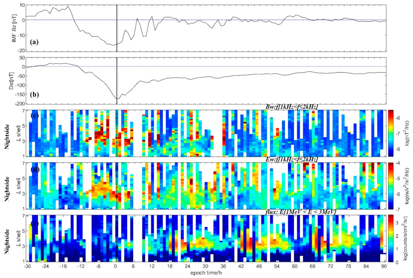
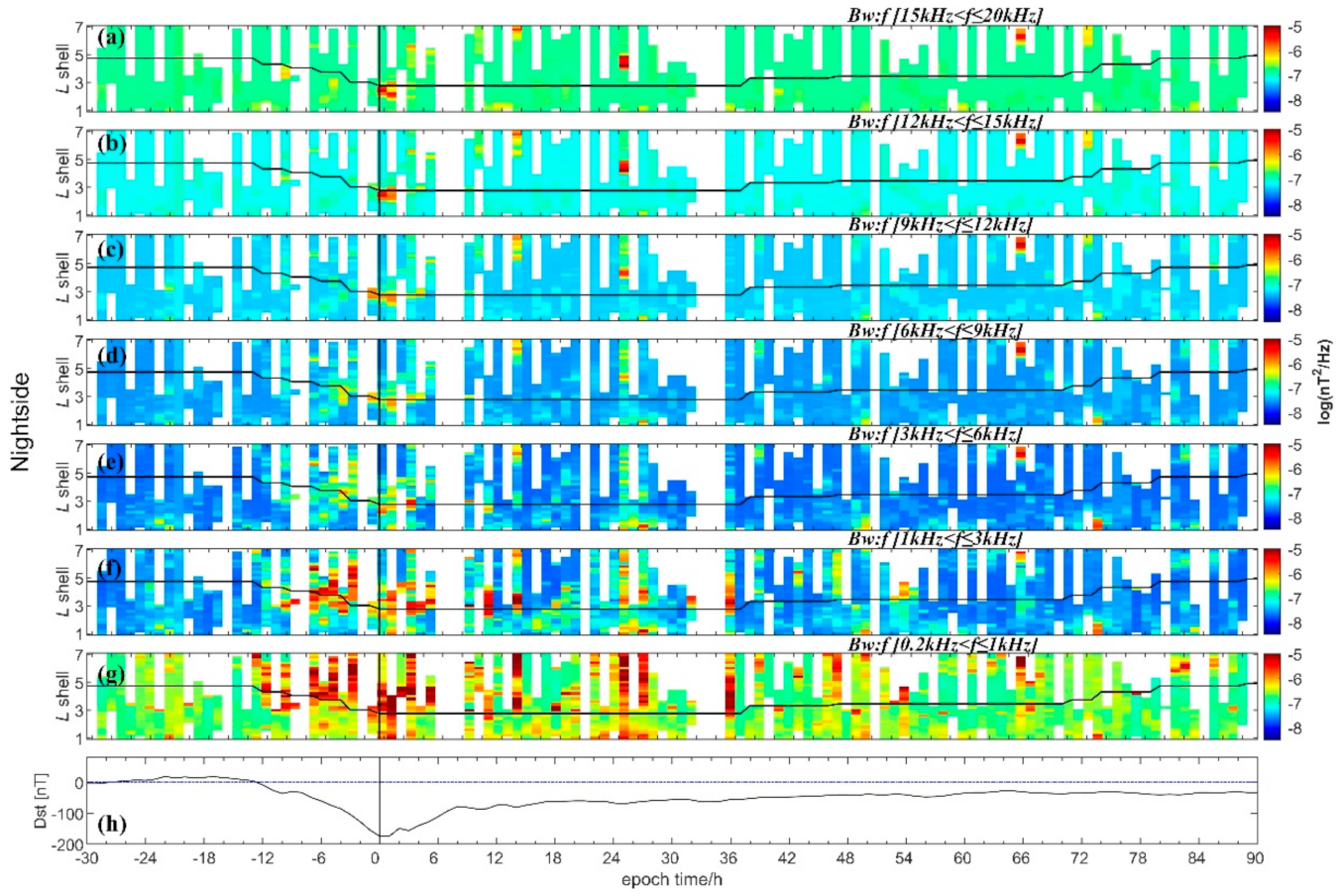
Figure 3 shows the results for the nightside ionosphere, where the ELF/VLF wave activities and electron fluxes also showed a close correlation of the different storm phases, though with a relatively weaker intensity than the dayside. It is interesting that in the nightside ionosphere, the waves at 1 kHz < f < 2 kHz were predominantly enhanced during the main phase in contrast to the ones at dayside; this feature is worth further exploration after more storm cases are accumulated.

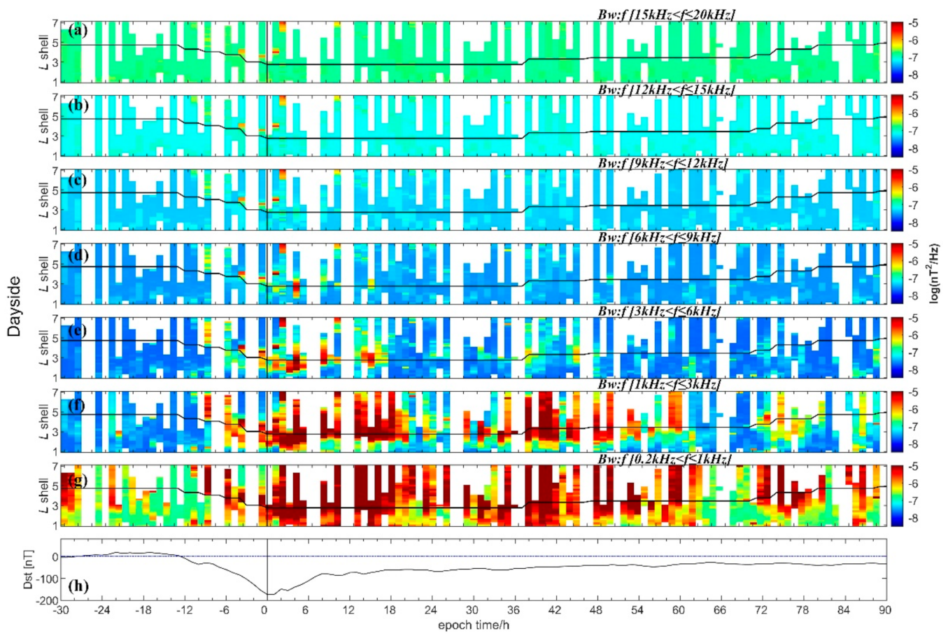
To further depict the temporal and spatial distribution of the wave activities of all the ELF/VLF frequency bands, we divided the electromagnetic field measurements into seven frequency bands: 0.2–1 kHz, 1–3 kHz, 3–6 kHz, 6–9 kHz, 9–12 kHz, 12–15 kHz, and 15–20 kHz. By using the same method from Figure 2, the average PSD values of each band from each orbit were computed and binned as a function of L shell values in a step of 0.2 L, with a time interval of 1 h in the epoch time period from t₀ − 30 h to t₀ + 90 h. Similar for the energetic electrons, the fluxes from the six energy bands were integrated: 0.1–0.5 MeV, 0.5–1 MeV, 1.0–1.5 MeV, 1.5–2.0 MeV, 2–2.5 MeV, and 2.5–3 MeV.

Figure 4 and Figure 5 show the results of ELF/VLF waves in the magnetic field from the day and night side ionospheres, respectively. In Figure 4 and Figure 5, the black vertical dashed lines denote the reference epoch time t₀. It can be seen that the arrival of an ICME at the magnetopause location directly led to strong ELF/VLF wave activities in the ionosphere. Specifically, before the ICME hit the magnetopause (t < t₀ − 16 h), the ELF/VLF wave activities at all frequency bands were relatively quiet. At the early stage of main phase (from t₀ − 16 h to ~t₀ − 4 h), the ELF/VLF waves were mainly excited at frequencies below 6 kHz. However, from the near-end main phase to the early recovery phase (from t₀ − 6 h to ~t₀ + 6 h), the wave activities significantly grew up in the entire frequency range from 0.2 to 20 kHz. During the long recovery phase, the wave enhancements mainly occurred below 6 kHz. These results from the CSES were consistent with our previous statistical analysis for CME-driven storms based on DEMETER observations [9].

Figure 5 shows that the nightside wave activities were weaker than those on the dayside. They also predominantly appeared at frequency below 3 kHz, and the phenomenon of the whole frequency band enhancement only appeared during the hours when the Dst reached its minimum values. The results of the electric field are not presented here, partially because they showed very similar features to those seen in the magnetic field and partially because there were high noises over the equatorial area that originated from instruments or satellite platforms (see the strong horizontal enhancement denoted by black rectangles in Figures 8 and 9 in Discussion Section).

We also estimated the location of the plasmapause by using the empirical linear model of O’Brien and Moldwin [45], which was based on the magnetic indices Kp and Dst values. According to that model, the plasmapause (denoted by the black curves superposed on the plots in Figure 4 and Figure 5) was significantly compressed during the storm time from L shell values of ~5 to ~3. According to the estimated plasmapause location, it can be said that the strong wave emissions at the frequencies below 6 kHz mainly occurred at a broad L shell extension (covering the L shell from ~1 to 7), both inside and outside the plasmapause; meanwhile, waves at frequencies higher than 9 kHz mainly appeared outside the plasmapause (L shell ~3 to 7), which means that waves in this portion of the spectrum mainly appeared in the radiation belt (more likely in the outer radiation belt).

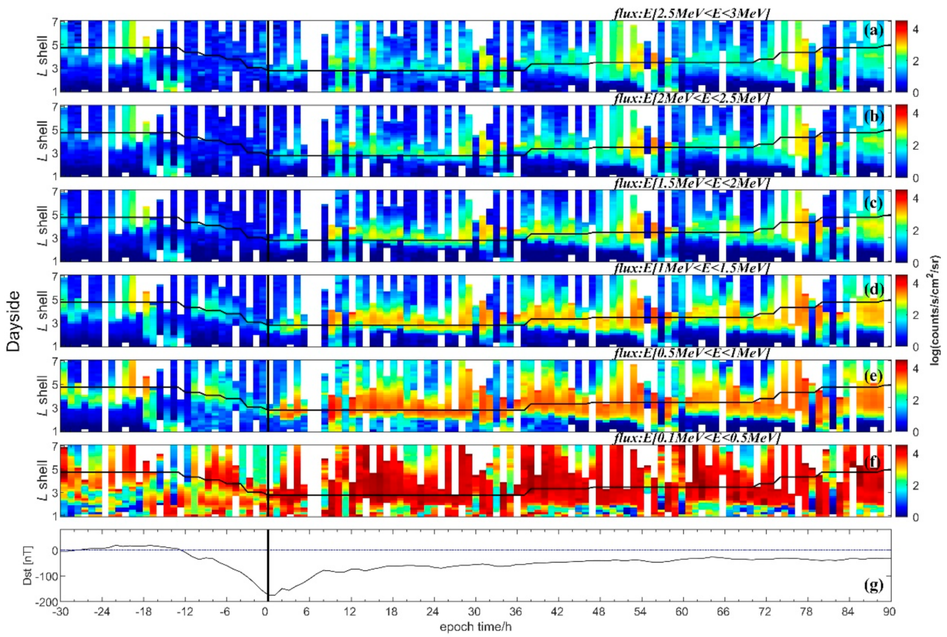
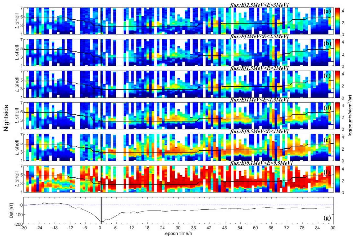
Figure 6 and Figure 7 show the temporal and spatial evolution of energetic electron fluxes at energies from 0.1 to 3 MeV in the day and night side ionospheres, respectively. During the main phase of the storm, the electron flux at E < 1 MeV intensely increased, but the ones at higher energy level E > 1.5 MeV decreased (see t = −12 h to 0 h). Subsequently, during the recovery phase of the storm, when the solar wind parameters and the Dst index were returning back to their nominal level, the fluxes at E > 1.5 MeV got enhanced to about 2 orders higher than those at the pre-storm values. Features in electron flux variations during storm evolution were consistent with earlier DEMETER observations in storm time [18].

Clearly, the precipitating flux increased with the geomagnetic activity level, with the primary maximization out of the plasmapause under active conditions. Specifically, sub-MeV (below E > 1.5) electrons showed strong enhancements across the whole storm time on both the day and night sides, as well as both inside and outside the plasmapause; however, for E > 1.5 MeV, the fluxes were mainly enhanced over the plasmapause.

4. Discussion

We present two half-orbit observations from the CSES as examples to discuss the exact electromagnetic environment in the ionosphere under geomagnetic quiet (Figure 8) and disturbed conditions (Figure 9).

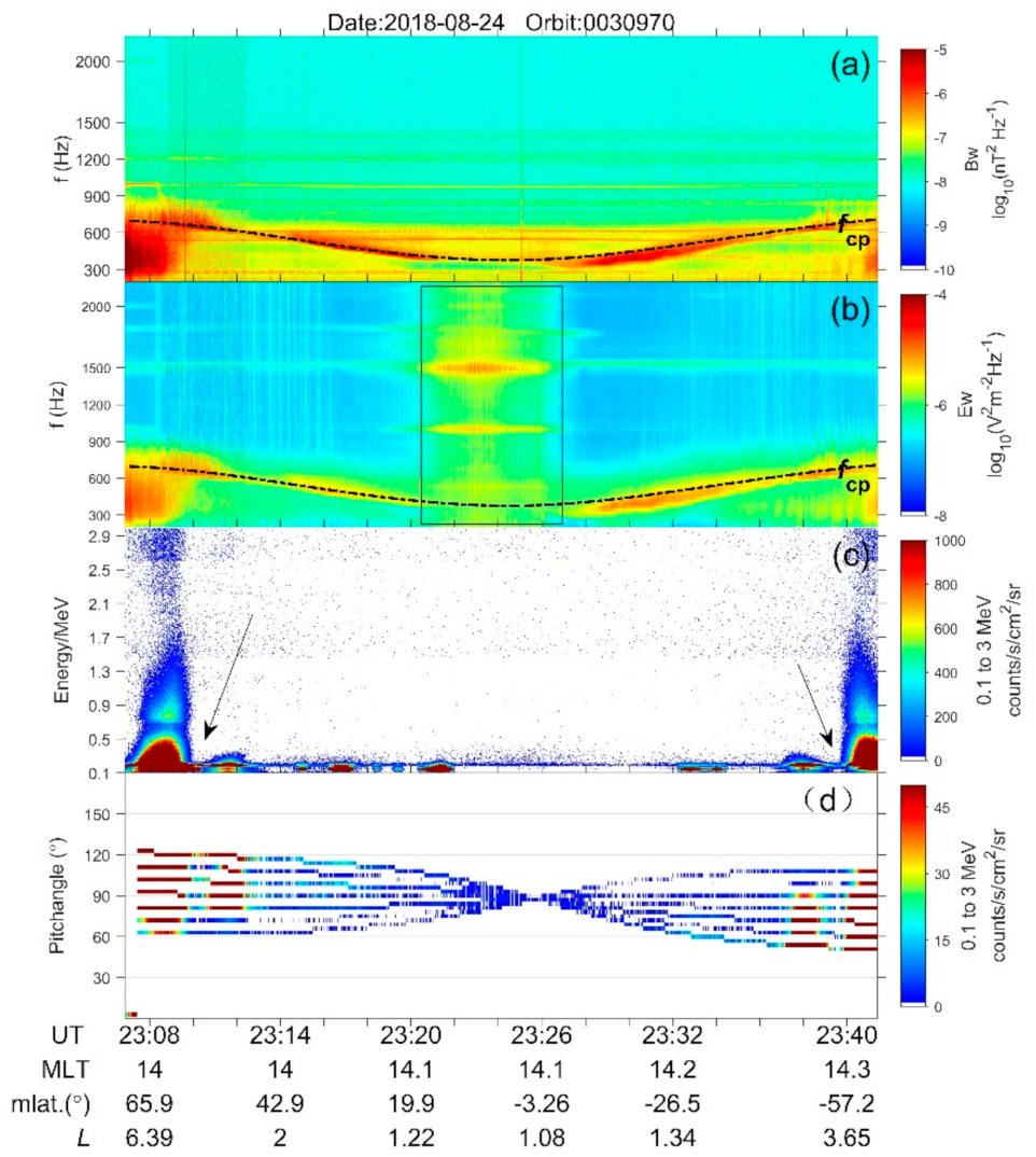
Figure 8 shows some typical half-orbit data of the CSES under a quiet space weather condition recorded by orbit No. 0030970 on 24 August 2018 (denoted by the vertical line Figure 1). The ELF/VLF waves are presented by the PSD values of the magnetic and electric fields (Figure 8a,b), respectively. The overlapping dashed curves represent the local proton cyclotron frequency f_cp, which was computed by the total magnetic field values provided by the HPM onboard the CSES.

From the energy spectrum of energetic electrons at 0.1 MeV < E < 3 MeV (Figure 8c), the outer/inner radiation belt is clearly visible (denoted by black arrows). In addition, we can see from Figure 8 that even under quiet space weather conditions at geomagnetic latitudes between ~40° and ~70°, there was a much higher level of ELF/VLF wave activity and energetic electron fluxes than the lower latitudes. Since the CSES is switched off at latitudes over ~65°, the region above 70° cannot be observed by it. Note that the electric field enhancement over the equatorial area (denoted by black rectangle in Figure 8b and Figure 9b) was due to artificial interferences from the EFD.

The variation of energy spectrum with respect to the local pitch angle distributions was further examined, as shown in Figure 8d, by using data from the nine silicon-slice units of HEPP-L onboard the CSES. Distinctly, at high latitudes over 50°, where ELF hiss waves appeared below 900 Hz, the energetic fluxes overwhelmingly got distributed at pitch angles from ~65° to 120°. The region within geomagnetic latitudes ±30° saw that the energetic electron fluxes dramatically declined, but the wave activities simultaneously enhanced at a frequency higher than f_cp.

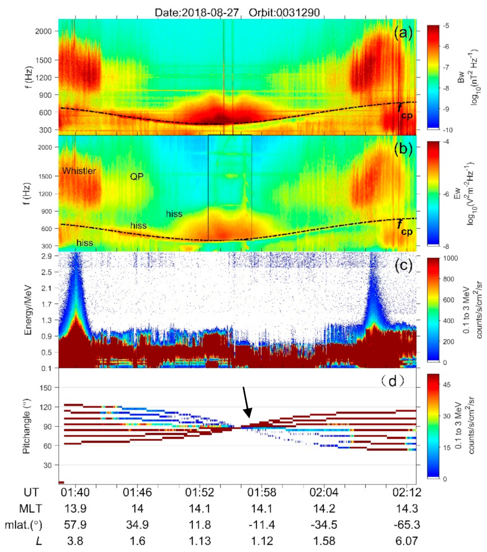
Figure 9 shows data from another half orbit that were recorded by orbit No. 0030970 during geomagnetic storm time on 27 August 2018 (recovery phase, denoted by the vertical solid line in Figure 1). Compared to the quiet condition in Figure 8, the CSES witnessed much stronger ELF/VLF activities and energetic electron fluxes enhancement under the active storm condition. Three typical electromagnetic waves could especially be identified, as follows:

(1) The ionospheric hiss waves that mainly appeared at frequencies around/below f_cp at geomagnetic latitudes from 20° (relatively weak) to 65° (predominantly) or at frequencies above f_cp to 800 Hz over the equatorial area with 20°, showing structure-less wave spectral property [22]; (2) the non-structured VLF waves at frequencies from ~1000 to 1800 Hz at high latitudes over 55°; and (3) the structured quasi-periodic structures (QP waves) at latitudes from ~35° to 50° [20].

For energetic electron fluxes, the CSES saw a direct enhancement of E < 0.9 MeV along the entire orbit trace, as well as increases of particles 0.1 MeV < E < 3 MeV at high latitudes around ~55° to 60°. It has to be noted that there were three silicon units that got saturated (see the arrow in Figure 9d); such saturation phenomena only occur under geomagnetically disturbed conditions, and data from the saturated silicon units were eliminated in the statistical analysis from Figure 6 and Figure 7.

In contrast to the quiet condition presented by Figure 8c, the slot region in Figure 9c is invisible; such disappearance can be ascribed to large scale precipitation extending to very low L shell region (L~2). In other words, the slot region was refilled by a large quantity of energetic particles that were probably accelerated or scattered through the ELF/VLF wave–particle interaction process in the outer radiation belt. The slot region refilling phenomena during this storm time was also investigated by Zhang et al. [26] based on a conjugated observations between the CSES and RBSP (Radiation Belt Storm Probes), and they found that the ELF/VLF whistler-mode chorus waves in the radiation belt could efficiently accelerate and diffuse the relativistic electrons at the extremely low L shell area in the ionosphere.

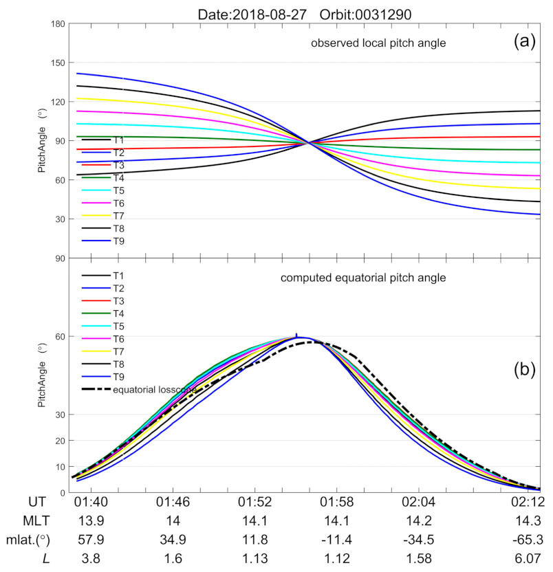
We further computed equatorial pitch angles by using the field-line tracing method based on the IGRF (International Geomagnetic Reference Field) model and the total magnetic field intensity recorded by the HPM onboard the CSES (see details in the work of Zhima et al. [20]). Figure 10a and Figure 11a show the observed local pitch angles, Figure 10b and Figure 11b the computed equatorial pitch angles for the half orbits of Figure 8 and Figure 9. It can be seen that for geomagnetic latitudes higher than ~40°, the computed equatorial pitch angles for the local observed particles were overwhelmingly lower than the equatorial loss cone (denoted by the thick black dashed lines in Figure 10b and Figure 11b), indicating these particles in the high latitude ionosphere as basically lost. However, at lower geomagnetic latitudes roughly within ±40°, we can see that certain particles were larger than the equatorial loss cone, indicating that they were most likely trapped instead of precipitation into this orbit space. It can be said that the CSES provided a good coverage of the energetic particle precipitations in the high latitude ionosphere.

After investigating a large amount of half orbit data (with every day of 62 half orbits) from 20 August to 4 September 2018, some basic features of energetic electron fluxes could be recovered: (1) under the quiet condition, the CSES could well depict the outer/inner radiation belt and the slot region (as Figure 8) well, whereas under disturbed conditions, such a region boundary was invisible due to large scale precipitation extending to very low L shells; (2) the regions poleward from geomagnetic latitudes 50° corresponded to the highest electron precipitation without any distinction between solar quiet or active conditions, and the regions below geomagnetic latitudes 30° generally got precipitations during the storm time and occasionally at quiet time; and (3) the ELF/VLF waves recorded by the CSES mainly included structure-less VLF whistler waves, structured quasi-periodic emissions, and structure-less ELF hiss waves. On the contrary, no whistler-mode chorus waves were found during this storm. Specifically, Figure 9 shows an example of the existence of whistler-mode waves with both non-structured (at the geomagnetic latitudes over 55°) and structured QP waves (at latitudes of 30° to 40°) at frequencies from 900 to 1200 Hz, as well as ELF hiss waves below the local proton cyclotron frequency f_cp.

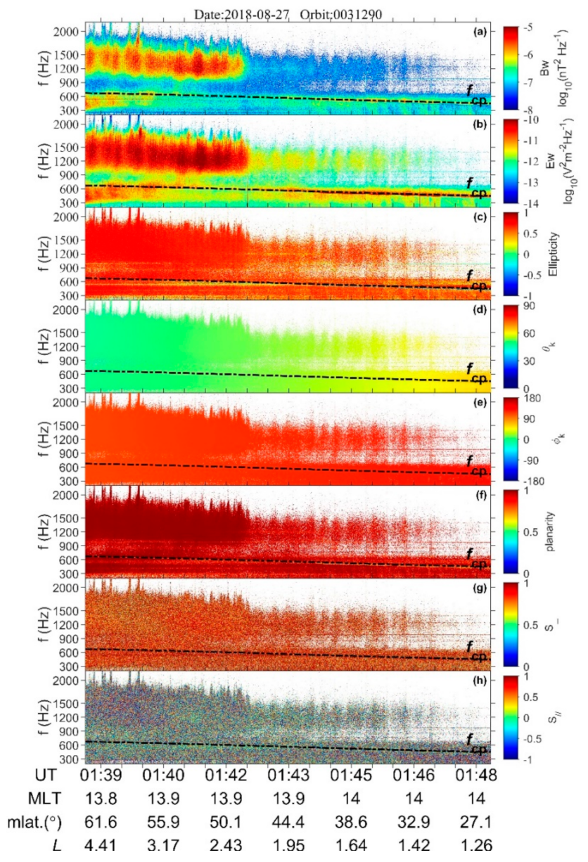
Thanks to the availability of waveform data below 2.5 kHz along the whole orbit trajectory, we could conduct a wave vector analysis to discuss the propagation features for these typical ELF/VLF whistler-mode emissions that occurred during the storm time. The wave propagation parameters for the ELF/VLF waves are shown in Figure 12, and they were computed by the singular value decomposition method [46] under the geomagnetic field aligned coordinate system (FAC) of the CSES (see details in Section 3.2 of the work of Zhima et al. [20]).

Figure 12 shows the wave vector analysis results for the ELF/VLF waves at northern high geomagnetic latitude regions (corresponding to the right part of Figure 9). The ellipticity value (Figure 12c), which is the ratio of the axes of polarization ellipse (+1 means right-hand circular polarization, −1 means left-hand circular polarization, and 0 means linear polarization), indicated that waves (900 Hz < f < 2000 Hz) and hiss waves (f < f_cp) were of the right-handed polarized whistler-mode and their wave normal angles (θ_k) (Figure 12d) generally varied in the range of around 40° to 65°. This suggested that waves obliquely propagated to the background magnetic field. Figure 12e shows the azimuthal angles (φ_k) (±180°: decreasing L shell direction; 0°: increasing L shell direction), which present values near 180°, suggesting that the observed ELF/VLF waves propagated towards the Earth direction (that is, in the decreasing L shell direction). The planarity of waves (Figure 12f), which represents the wave propagation mode, exhibited a value mostly equal to +1, meaning that the observed waves were coming towards the spacecraft as plane waves. The Poynting fluxes ($E\times H$) were computed by the six components of the electromagnetic waves [20]. It can be seen from Figure 12 that Poynting fluxes (S) mainly dominated in the perpendicular direction to the background magnetic field instead of the parallel directions.

According to Figure 12, the ELF/VLF whistler-mode waves obliquely propagated from the outer radiation belt towards the satellite along the Earth direction. Such peculiarity agreed with previous studies [17,29] that highlighted that in the high latitude ionosphere, these particles most likely propagate from the outer radiation belt and precipitate into the ionosphere (or into the atmosphere) as a consequence of their interactions with ELF/VLF waves. Zhima et al. [9] and Fu et al. [47] interpreted the generation of ELF/VLF waves in the ionosphere as mostly likely being due to the strong temperature anisotropy after solar wind energetic particle injections during storm time, which provides free energy for wave excitation to amplify the ELF/VLF waves in the upper ionosphere.

5. Conclusions

This study reports the temporal and spatial distributions of ELF/VLF wave activities and energetic particle enhancement in the mid-high latitude ionosphere during storm time based on observations from the SCM, EFD, and HEPP-L payloads onboard the CSES, which has been operating in low Earth orbit at an altitude of 507 km from February 2018 to present.

The 26 August 2018 intense storm resulted from an ICME event from the Sun, leading to strong ELF/VLF emissions and energetic electron precipitations in the upper ionosphere. The superposed epoch analysis for ELF/VLF waves and particles indicated that before the ICME hit the magnetopause, the wave activities and particle precipitation were relatively weak in the ionosphere, and the climax of wave excitations mainly appeared during the near-end main phase and the early recovery phase. Regarding frequency, the waves at frequencies below 6 kHz mainly occurred at the early stage of the main phase; a broad frequency band wave from f_cp to 20 kHz was remarkably excited from the near-end main phase to the early recovery phase. During the long period of the recovery phase, the wave enhancements mainly occurred below 6 kHz. The wave activity in the nightside ionosphere showed a good correlation with the evolution of the geomagnetic storm, but the amplitude of such was weaker than that on the dayside its spatial scale was also narrowly distributed.

The energetic precipitating fluxes increased with geomagnetic activity and reached their maximum during the early recovery phase, as primarily observed outside of the plasmapause. The energetic electrons at an energy level below 1.5 MeV got strong enhancements during the entire storm time on both the day and night side (relatively stronger than the ones on the dayside), and they also appeared both inside and outside the plasmapause; for particles E > 1.5 MeV, the fluxes mainly got enhancement from outside the plasmapause.

An investigation into a large amount of half orbit data in the whole time period showed that under the quiet condition, the CSES depicted the outer/inner radiation belt in the slot region well, whereas under disturbed conditions, such regions were invisible and dominated by precipitations of E < 1 MeV all along the CSES orbit space. The regions poleward from the geomagnetic latitude of 50° corresponded to the highest electron precipitation regardless of the quiet or active conditions; the regions equatorward below 30° were usually enhanced during the storm time and occasionally during the quiet time.

The ELF/VLF waves recorded by the CSES during the storm time mainly included structure-less VLF waves, structured ELF/VLF quasi-periodic emissions, and non-structured ELF hiss waves. A wave vector analysis indicated that the ELF/VLF waves were right-handed polarized whistler-mode waves, and they obliquely propagated from some area higher than the satellite (most likely from the outer radiation belt) to the Earth direction.