Determination of Zenith Angle Dependence of Incoherent Cosmic Ray Muon Flux Using Smartphones of the CREDO Project

Abstract

The Cosmic-Ray Extremely Distributed Observatory (CREDO) was established to detect and study ultra high-energy cosmic ray particles. In addition to making use of traditional methods for finding rare and extended cosmic ray events such as professional-grade Extensive Air Shower (EAS) arrays, as well as educational ‘class-room’ detectors, CREDO also makes use of cameras in smartphones as particle detectors. Beyond the primary scientific goal of the CREDO project, to detect Cosmic Ray Ensembles, is the equally important educational goal of the project. To use smartphones for EAS detection, it is necessary to demonstrate that they are capable of effectively registering relativistic charged particles. In this article, we show that the events recorded in the CREDO project database are indeed tracing incoherent cosmic ray muons. The specific observed distribution of zenith angle of charged particle direction corresponds to that expected for muons. It is difficult, if not impossible, to imagine different mechanisms leading to such a distribution, and we believe it clearly demonstrates the suitability of smartphone-based detectors in supporting the more traditional cosmic ray detectors.

1. Introduction

The cosmic ray energy spectrum extends from below ∼100 MeV [1] up to ∼10${}^{20}$ eV [2]. The spectrum and composition of cosmic rays for energies up to the “knee” is compatible with diffusive shock acceleration mechanisms [3]. The maximum energy achievable in this shock acceleration process is at about PeV region [4,5]. The types of objects in the Universe that are able to accelerate particles at even higher energies are limited in number. In the case of ultra high-energy cosmic rays, it seems that there are few places capable of accelerating particles above ${10}^{20}$ eV: large scale shocks surrounding galaxy clusters, internal or external shocks of starburst-superwinds, Active Galactic Nuclei (AGN) or Gamma-Ray Bursts, AGN flares, jets, magnetars, lobes of giant radio galaxies, see [6] for a review of these. Some of the exotic models can be verified by searching for new, rather unexpected behavior of cosmic rays at the highest energies. One of them is a focus of the Cosmic-Ray Extremely Distributed Observatory (CREDO) Collaboration. This global approach allows the testing of hypothesized events of ultra-high energy cosmic ray ‘bunches’ observed as simultaneous Extensive Air Showers (EAS) over the entire exposed surface of the Earth: so-called Cosmic Ray Ensembles (CRE) [7,8,9]. Such a phenomenon has never been seen, but there are several models under which such an event is a possibility.

To observe such events, a system operating on that global scale is required. Due to the extreme geographical scale of the data acquisition, the CREDO Collaboration makes use of non-expert science enthusiasts. They participate in research with their own mobile devices equipped with the CREDO Detector application [10] which enables detection of ionizing radiation using the CMOS sensors.

(with their own smartphones). The idea of using an array of smartphones as cosmic ray/muon detectors is a quite recent possibility—as the density of smartphones per squared km is a significant feasibility parameter [11]. This was realized, to some extent, by the DECO [12,13] and CRAYFIS [14] projects, and even in muon flux determination measurements [15], but at the same time the quality of individual data as well as the idea itself was criticized [16,17].

The possibility of registering an EAS by detectors of such small active area requires a large number of smartphones concentrated in a relatively limited footprint. The typical EAS array of contemporary cosmic ray experiments consists of hundreds of detectors exceeding several square meters in size (e.g., KASCADE in Karlsruhe [18]; MAS at Mount Chacaltaya [19], or GRAPES at Ooty [20]).

To effectively study cosmic ray physics at energies of 10${}^{19}$ (10${}^{20}$) eV, the density of smartphones (constantly working taking “dark” frames) should be 5000 (1000) per km${}^2$ [17] or as few as 400 [11], which remains a challenging scale of detectors. To have an EAS smartphone array comparable to the large experiments like Pierre Auger Observatory or Telescope Array, we would require millions of phone cameras across an area of thousands of square kilometers, all permanently ‘on’. The goal of registering every EAS from each CRE at close to 100% effectiveness, and measuring its characteristics (total number of particles, their distribution with respect to shower core, and incoming direction) is simply unfeasible. However, it may be possible to detect some signal from any CRE using a coincidence across very distant sets of detectors (smartphones).

Another noted challenge is the contamination of smartphone camera signals by sources other than cosmic ray. In principle, this includes the housing of the camera itself, as a smartphone is not made to be “low radiation background”. It typically contains many radioactive nuclei of isotopic composition similar to the Earth’s crust, which constantly decay to give signals in the semiconductor camera matrix elements. The U, Th, and K nuclei present, for example, in the walls are obvious sources of the unwanted background [16]. Ultimately we need to determine experimentally whether smartphones can be used as cosmic ray particle detectors, or if this background noise removes the possibility of measurement in practice.

To address this issue, we approach it from the opposite case. We make the assumption that particles, other than cosmic muons, do not have a characteristic distribution; unlike the very well known distribution demonstrated by single cosmic ray muons. In Section 3, we will show that long traces fit perfectly to the known muon relation, so we conclude that other sources of charged particle contamination in this particular region is small, but on the other hand, for short traces it may be significant and cannot be eliminated in practice.

2. Registration and Analysis of the Smartphone Recordings

The cosmic ray CREDO Detector application for smartphones is available freely at Google Play. The active users send their records to the CREDO database. They have access in turn to all the data from other users to download, study, and analyze for their own Citizen Science efforts. In the CREDO database, there are approximately a million images registered with the smartphone camera’s lens obscured.

Such recorded images should consist mostly of black pixels. When this condition is met, the CREDO Detector application starts working. If a particle of secondary cosmic radiation, muon (or possibly a particle of local radiation source), passes through the active layer of the smartphone camera it will stimulate some of the pixels. A few to several dozen pixels, distributed in a cluster of shapes that range from circular to extended lines, should then appear brighter on the roughly homogeneous black background. In one 24-h period there can be anything from one to several hundred detections.

Events in which very long traces are visible can potentially be the tracks of cosmic ray muons that passed through the camera at large angles. This possibility is, in theory, easily verifiable. The zenith distribution of such incident angles of single incoherent muons is well established, and is actively measured by small, even portable, muon telescopes often created and operated by students [15,21,22,23,24] as a demonstration of their detectors. In this paper, we will show that the majority of CREDO registered events are due to real muons with a recovered zenith angle distribution as expected.

The data used to obtain the results presented below consist of more than 100,000 CREDO database registrations obtained by one (very active) user with only one camera. The CREDO application draws a lot of power, and practically can only be used for extended periods when connected to a charger. Therefore, the cameras actively connected to the CREDO network usually rest permanently in the same place, which means that once placed horizontally they remain in this position permanently, and we do not have to be concerned of blurring the distributions by uncontrolled changes in the camera matrix plane. The registrations are available as PNG files cropped from the whole camera frame to 60 × 60 pixels around the brightest pixel in the frame.

Some events in the database are caused by the single pixel noise signal near the edge of the camera, and the image does not consist of 60 × 60 pixels around the brightest pixel. This reduces the number of pictures used in the present analysis from $1\times {10}^5$ to $6\times {10}^4$. Examples are shown in the top row in Figure 1. Signals are roughly proportional to the ionization energy loss in the particular matrix pixels, but it should be noted that some corrections (unknown in practice) have been applied to the photos by the internal camera software. The box 2D-histograms are given in the middle row in Figure 1 which scale in size with the ionization energy. The bottom row is the process by which the main axis of the “muon tracks” are identified.

2.1. Determination of Noise

For each registered event, we determined the average dark pixel brightness and its standard deviation $\sigma$ using only regions far from bright pixels (these are either intrinsic ‘hot spots’ on the chip or from the suspected signal itself). This procedure was then repeated after removing the pixels which exceeded $2\sigma$ above the initially-estimated average. At this stage, all pixels containing (potentially) everything associated with the registration of a cosmic ray muons (and ’hot spots’) are omitted. Statistics from the, over 3000, remaining pixels in each frame allowed us to obtain a well-defined average brightness of dark pixels and its intrinsic variance. These are considered reliable values attributable to the noise in each recorded event.

2.2. The Elongation Axis

The next step in the analysis was to find the main symmetry axis of the track. First we selected all pixels that exceeded the threshold (equal to the previously estimated average signal of the dark pixel noise, plus 10× its finally determined standard deviation). We have confirmed that using a factor of 5 instead of 10 does not significantly influence the results, as the signal we observe is so much brighter than the average noise value.

For the selected pixels (i.e., those above the dark pixel threshold) we determined the ‘main axis’ of the track. There are, in principle, many ways to determine this, and we have tested several: inertia ellipses, the Hough algorithm line, the smallest sum of squared distances weighted by squares of the brightness, and even the brightness only. They all give very similar results as the images of the tracks in each picture are clear, and regardless of how they are linearized the ‘main axis’ of the track is (almost) always the same. The lines are shown in the bottom row in Figure 1.

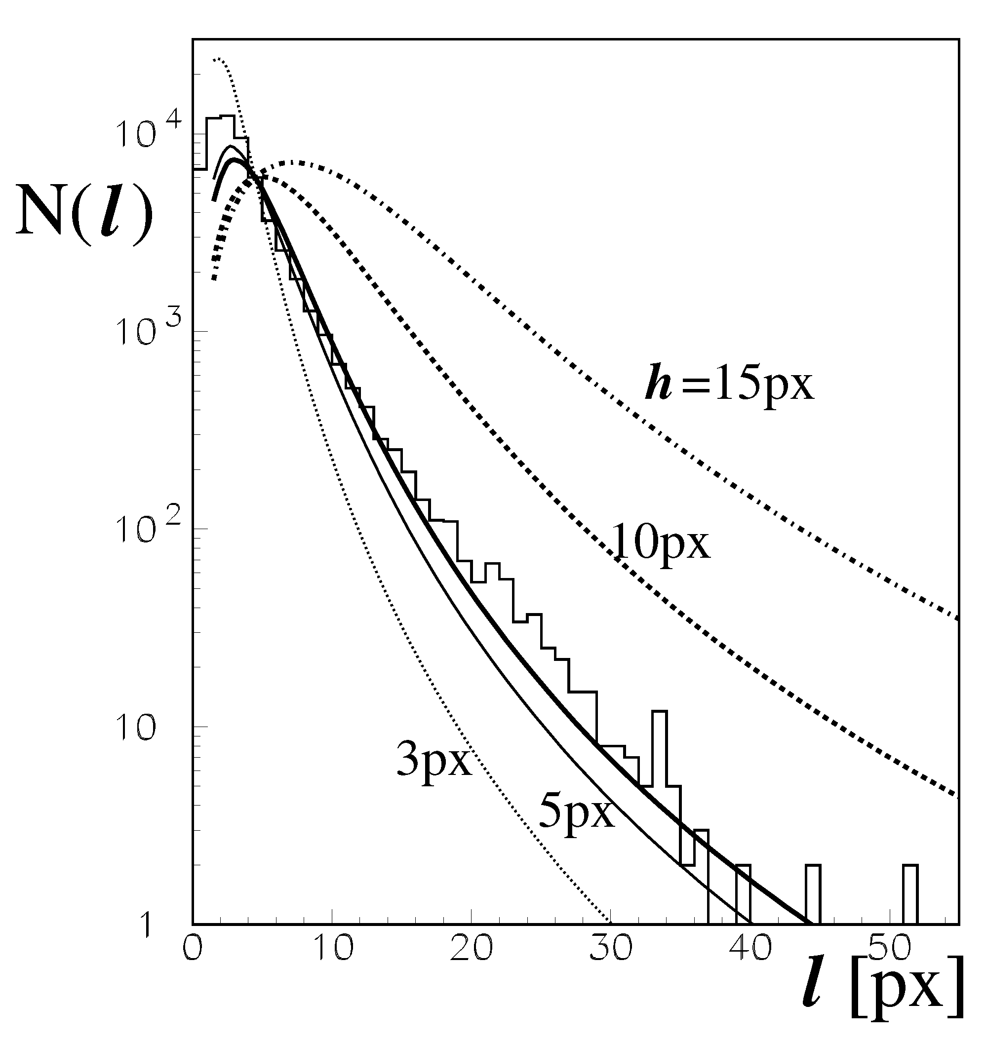
2.3. The Length of the Track

All pixels exceeding the threshold described in the section before are projected onto the newly-identified main axis of the analyzed trace. Assuming that the axis is the real main axis of the track the obtained histograms represent the ionization along the trace. The respective examples are shown in Figure 2. If we deal with a trace of a relativistic cosmic ray particle (muon), the signal pixels should have roughly the same brightness (with obvious geometric corrections). Such idealized situations are encountered only rarely, however.

The ends of the track were found by tracking to the left (and to the right) from the point with the highest projected brightness, until the signal values become smaller than limit chosen by trial and error. We defined this limit as a fraction of the second projected brightest bar in the histograms. The values are shown in Figure 2 as dashed lines. Using just the brightest histogram bar value the procedure could be subject to fluctuations to the larger extent. The value of this fraction was selected comparing the results of the algorithm with the subjective perception of the observer. Eventually, the value of 30% was established.

In some cases there is a very small gap in the trace, as it seen in the first (top left) image in the example shown in Figure 1 and Figure 2a, where we can guess that the real track continues on both sides of the two histogram bins with the summed brightness value below the threshold line (Figure 2). Other times, the gap can be quite long as the third column exemplifies, where it extends over 5 histogram bins (Figure 2c). The question then arises if we are dealing with a single track, or a random contamination of unknown origin. Before we attempt to answer this question, we first have to define some relevant variables.

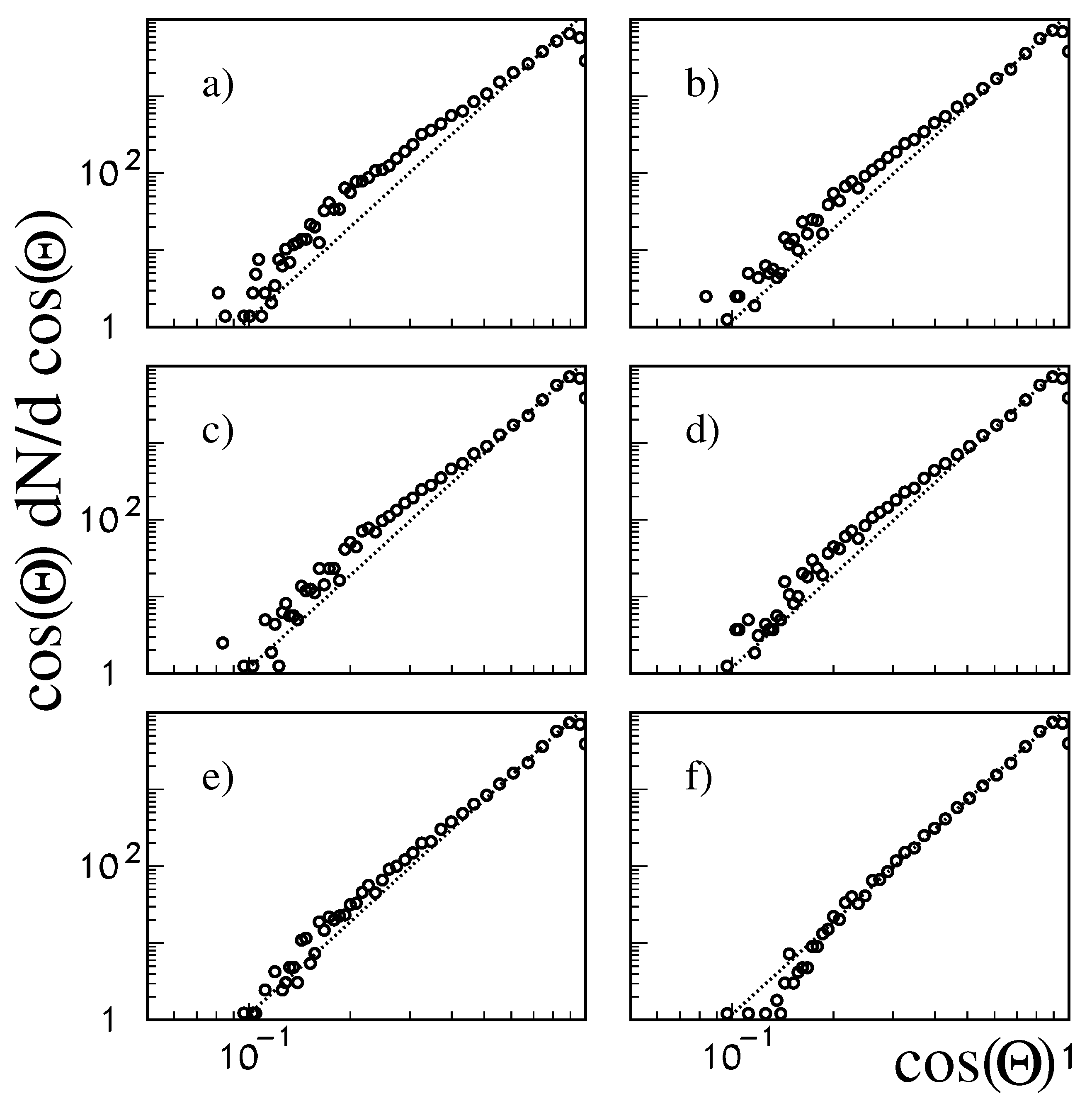
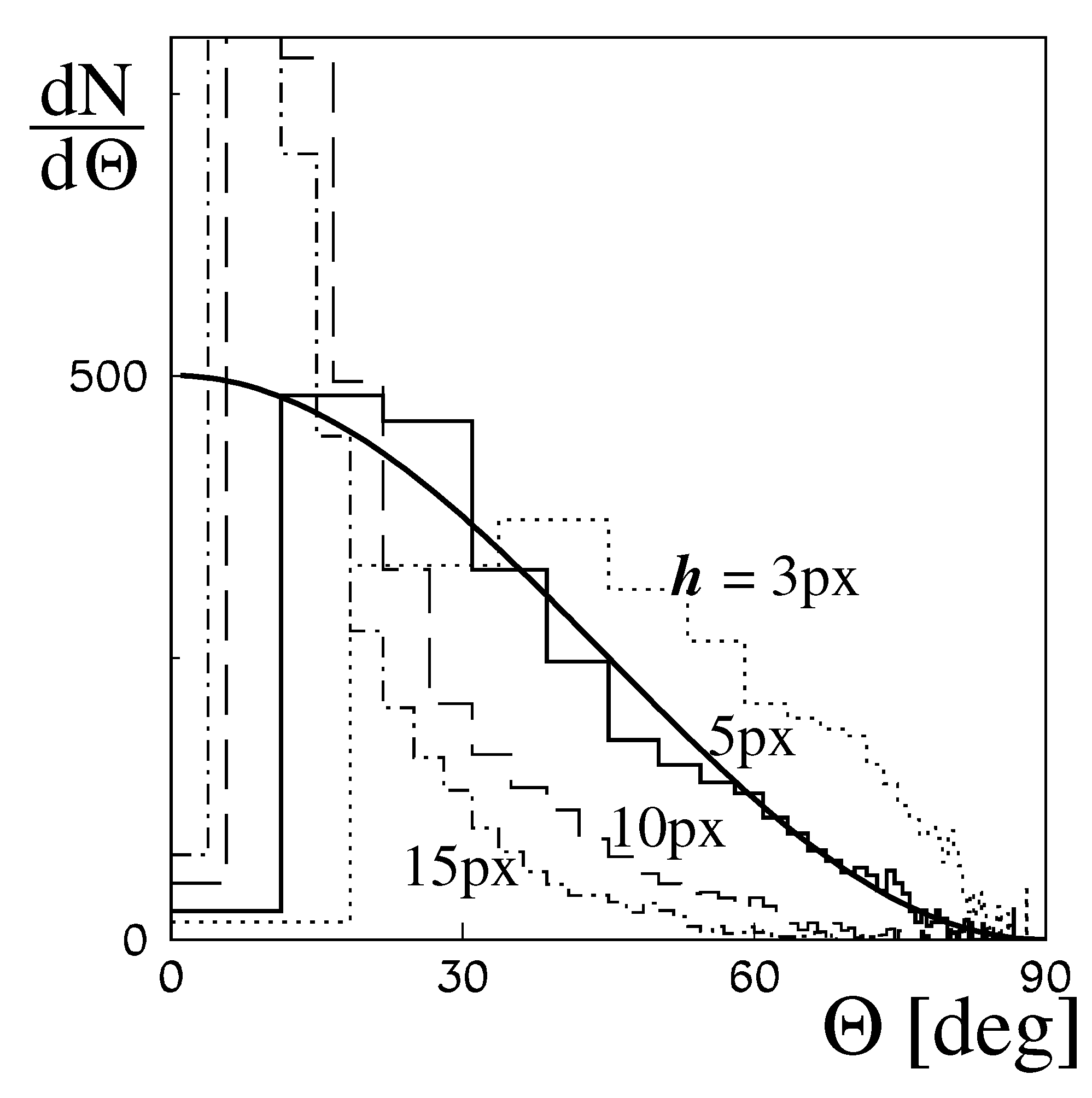
2.4. Zenith Angle of the Particle Track

The zenith angle of the particle track $\mathsf{\Theta }$, if we assume that it is indeed the trace left by a particle passing through the entire photosensitive layer of the camera, is naturally determined by the track length observed in the camera plane and thickness of the photosensitive layer of the camera matrix itself.

$$\mathsf{\Theta }=arctan\frac{l}{h}$$

(1)

where l is the track length, and h is the depth of the sensitive layer of the matrix in the smartphone camera. Measuring the track length distribution, we can obtain the zenith angle dependence of the observed particle flux. It can then be compared with the prediction of a model. For example, if we assume that particle flux reaches the Earth surface isotropically, the zenith angle distribution observed by the flat horizontally placed detector will be of the form $dN/d(cos(\mathsf{\Theta }\left)\right)\sim cos\left(\mathsf{\Theta }\right)$. With non-isotropic, but still a power-law in the variable $cos\left(\mathsf{\Theta }\right)$, the simple power-law form of the observed distribution is expected.

The cosmic ray single muon zenith inclination angle distribution has been known for nearly 80 years [25,26] and many different measurements confirm that it is quite accurately described as

$$f\left(\mathsf{\Theta }\right)={cos}^{\gamma }\mathsf{\Theta }$$

(2)

with the index of $\gamma \sim 2$. We will use this simple relation to test our algorithms for observed track identification.

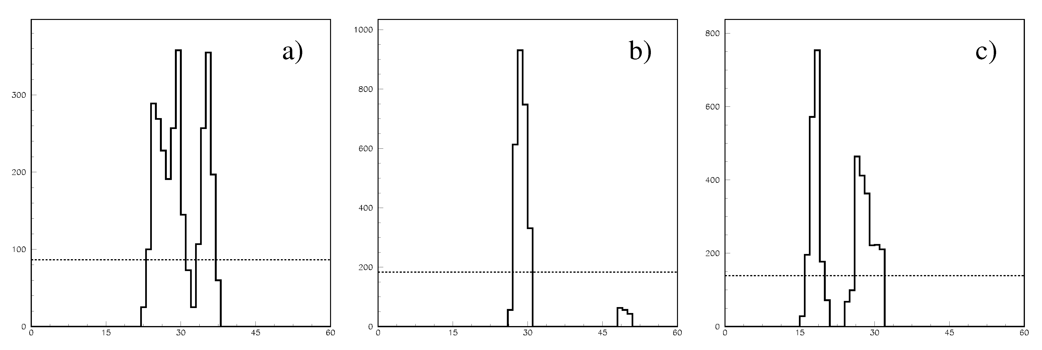
2.5. The Track Length Determination Algorithms

There is, in general, high subjectivity to the interpretation of the images of long tracks with complex and complicated traces. Thankfully, these cases are rare, but they affect the tails of the track length distribution. The algorithm for the track length determination is especially sensitive to the treatment of the multi-component pictures, when the gaps in the traces are seen.

After the projection of the pixel brightness along the identified track’s main axis, the gaps in the histogram are clearly visible (see Figure 2) and the question then arises where the real particle track ends, if it is, of course, the real particle track in the first place. This question can be further expanded into more detailed ones: how long can the gaps be allowed in a single track, and how to treat the cases with the longer gaps. In principle, we can accept just the longer length regardless, or we can reject the entire frame from the track length distribution estimation procedure. We have tested several of these possibilities, noting as before that, with the appropriate method, the true cosmic ray muon tracks are expected to follow the power-law distribution of $cos\left(\mathsf{\Theta }\right)$.

The results of the six procedures are shown in Figure 3. The respective $cos\left(\mathsf{\Theta }\right)$ distributions are shown there. To convert from l to $\mathsf{\Theta }$ (or to $cos\left(\mathsf{\Theta }\right)$), the depth of the camera’s photosensitive layer is set here, for the time being, to 5 px. For simplicity we will, hereafter, measure all distances, and the track length, as well as the thickness of the matrix sensitive layer, using as a unit a single matrix pixel size (px). This is quite a natural unit if we are dealing with the same camera, as is in the case of the present work. The thickness of the photosensitive layer will be considered later in this paper.

We explore in detail below the tested algorithms using the examples in Figure 3. Initially, we explore the steps within the least restrictive algorithm:

(a)

acceptable gaps in the histogram tracks are of length up to 4 px (as shown in Figure 2) but exactly one track is seen in the picture,

(b)

as above up to 4 px gaps are accepted but ’multiple track’ events are included.

In the middle row of Figure 3, we compared results of algorithms for ’multiple track’ cases

(c)

allowing events with large gap (up to 5 px) in the track,

(d)

only the small gap (only below 3 px) is acceptable.

In the lower row of Figure 3, we present results for single-track cases and a very strong criterion for the gap length in the track

(e)

only 1 px long gaps, at most, are accepted,

(f)

no gaps at all are allowed.

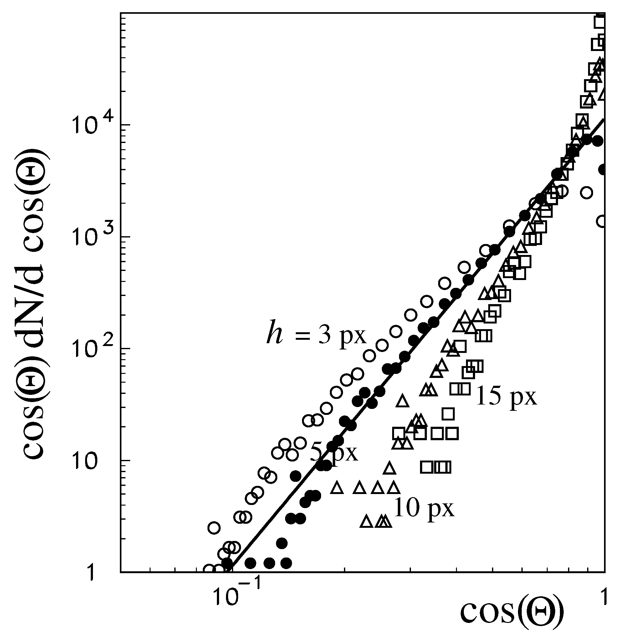
Most noticeably, we can see that the details of the algorithm used are primarily responsible for determining the very long tracks (large zenith angles) distribution. Rejections of the multiple tracks events affect mostly those very long tracks, which are about 1% of the overall population. Then the statistics of all plots in Figure 3 is very close to the total count of 60,000 regardless.

We can now compare in detail the measured distributions obtained using the six algorithms described above, restricted to the $40°<\mathsf{\Theta }<70°$ region. The upper limit is based on a simple statistical argument and has practically no influence on the results of the fitting procedure. The lower limit of 40 degrees is related to the additional smoothing of the short track lengths due to the dimensions, and even the geometry, of the camera pixel matrix. An exact zenith track should give a track length of zero px, a slightly inclined track may give a track length of 1 px (or even $\sqrt{2}$), if it passes through an edge. In addition, the actual structure of the camera matrix is obviously unknown (detailed pixel shapes, spacing, etc.). All of this makes the contents of the first few bins of the path length histogram difficult to interpret and thus difficult to correct for all these effects. It should also be remembered that events in which only one pixel signal is above the threshold are rejected by the acquisition software. In the limited region, we see a near linear behavior in log × log scale, thus the power-law of the $cos\left(\mathsf{\Theta }\right)$ distribution. The most restrictive criteria (case Figure 3f) is determined to be the most conservative, and most suitable.

To be more specific, we calculate values of ${\chi }^2$ comparing the measured distribution with predictions for cosmic ray muons (using $h=5$ px). In the angular range $40°<\mathsf{\Theta }<70°$ there are 10 histogram bins and the respective six values are: 723, 278, 302, 237, 99, and 36. It should be remembered that these are not results of any minimization procedure, and normalizations were fixed in each case at the point of $\mathsf{\Theta }\approx 40°$.

Henceforth, we will use the most restrictive algorithm to determine the track lengths.

3. Results

With the selected algorithm, we study the distribution of the length of the tracks recorded on smartphone photos stored in the CREDO database, in order to determine whether it is consistent with the zenith angle distribution of the muon (∼${cos}^2\left(\mathsf{\Theta }\right)$). The degree of the expected accordance will show the confidence of using the smartphone cameras as cosmic particle detectors.

We start detailed studies with the distribution of the track length as it is shown as the histogram in Figure 4.

Predictions assuming that we are dealing with the cosmic ray muons with the known zenith angle distribution are also shown. These distributions differ for different values of the camera photosensitive layer thickness h. The thickness of the particular camera we used in this work is not known precisely, leaving the value of h to some extent a free parameter which can be constrained by the data itself. We present here results for 3 px, 5 px, 10 px, and 15 px and the predictions of the best fitted value of h. Details of the fitting procedure are given below.

In Figure 4, we see that the measured distribution is close to the predictions for a width (h) close to 5 px. However, it can be seen that this agreement is not perfect at both long track lengths, as well as for very short lengths. Regardless, the distribution of track length presented in Figure 4 can be converted to the zenith angle distribution (assuming we have captured cosmic ray particle traces). Zenith angle distribution is more suitable for studying cases of small angles (short trace lengths). In Figure 5, we present the comparison between the predictions obtained using different values of h.

The length of the track determined with the algorithm described above, if expressed in single pixel size (px), is, by definition, an integer number. For small values of h, which are expected in modern smartphone cameras, the measured zenith angle, given by Equation (1), would have to be discrete numbers. The resolution for small angles, at which most particles arrive at, is very limited. For larger angles, longer tracks, where the resolution of a determined angle is superior, the flux is substantially smaller, thus the simple zenith angle is not the best variable to study.

However, Figure 5 also suggests that for small angles, where most of the events occur, the matrix sensitive layer thickness is close to 5 px. While the short track discrepancy may be due to the measurement uncertainty, the discrepancy for large l values can be mitigated by selecting an appropriate value for the photosensitive layer thickness h.

The ${\chi }^2$ minimization procedure was used on the $cos\left(\mathsf{\Theta }\right)$ distribution shown in Figure 6 where results are obtained for different assumptions about the thickness of the photosensitive layer parameter h. We have compared it with the expected power-law spectrum with a slope corresponding to the distribution of cosmic ray muons. This slope is given by the thick line in Figure 6.

The distribution of the variable $cos\left(\mathsf{\Theta }\right)$ illustrates very nicely the behavior of the long and very long (about horizontal) tracks. Due to the problems with short tracks we have fixed the normalization at the point corresponding to the zenith angle of ∼$40°$ and used only bins corresponding to $40°<\mathsf{\Theta }<70°$. The minimum value of ${\chi }^2$ for 10 normal degrees of freedom was found to be 6.7 for the h = 5.7 px. This best solution found is shown in Figure 4 and Figure 6 by the thick solid line.

It should be noted here that in [13,27] a similar analysis was performed and the authors concluded that the camera they used had a matrix sensitive layer thickness (termed in their work the “depletion thickness”) of $29.2\pm 1.5$ px, greatly exceeding our measurements. The more recent measurements of [15] have results that are compatible with a thickness of the camera matrix close to 3 px. The former analysis was based on as few as 200 registered events, the later on approximately 230 tracks. The analysis presented in this paper is based on about 60,000 tracks and hence we believe represents a significant advancement in the field.

4. Summary

We have explored the method of analyzing pictures taken by a smartphone camera with the lens obscured. In these instances, some tracks are clearly visible exceeding the dark frame camera noise. In most cases, the determination of this track length is not a significant challenge. Different methods of determining the track’s main axis were tested, and lead to near indistinguishable results overall. There was some uncertainty for very long tracks corresponding to incoming particle with zenith angles greater than 80$°$ (almost horizontal). We removed these associated ambiguities by eliminating ‘long gap events’, showing this ultimately to be a satisfactory solution.

The analysis of the track length distribution with the camera sensitive layer thickness considered as a ‘free parameter’ adjusted to the observations, agreed well with the results obtained found with a reasonable value of about 5 px ($5.73\pm 0.04$ px), where the unit of measure (px) is the size of the individual camera matrix pixel.

5. Conclusions

We have shown that the distribution of the zenith angle of particles responsible for the emergence of tracks in the smartphone captured images is in agreement with the expected distribution of the zenith angle of single, incoherent, cosmic ray muons. This confirms the idea that smartphones can operate in practice as ’particle pocket detectors’, sensitive to charged relativistic cosmic particles and hence can be used effectively by the CREDO Project and other similar initiatives.

References

1. Neronov, A.; Malyshev, D.; Semikoz, D.V. Cosmic-ray spectrum in the local Galaxy. Astron. Astrophys. 2017, 606, A22. [Google Scholar] [CrossRef]
2. Aab, A.; Abreu, P.; Aglietta, M.; Albury, J.M.; Allekotte, I.; Almela, A.; Castillo, J.A.; Alvarez-Muniz, J.; Batista, R.A.; Hahn, S.; et al. Measurement of the cosmic-ray energy spectrum above 2.5 × 10¹⁸ eV using the Pierre Auger Observatory. Phys. Rev. D 2020, 102, 062005. [Google Scholar] [CrossRef]
3. Hörandel, J.R. Models of the knee in the energy spectrum of cosmic rays. Astropart. Phys. 2004, 21, 241–265. [Google Scholar] [CrossRef]
4. Bell, A.R. Cosmic ray acceleration. Astropart. Phys. 2013, 43, 56–70. [Google Scholar] [CrossRef]
5. Zhang, Y.; Liu, S. The Origin of Cosmic Rays from Supernova Remnants. Chin. Astron. Astrophys. 2020, 44, 1–31. [Google Scholar]
6. Batista, R.A.; Biteau, J.; Bustamante, M.; Dolag, K.; Engel, R.; Fang, K.; Kampert, K.-H.; Kostunin, D.; Mostafa, M.; Murase, K.; et al. Open Questions in Cosmic-Ray Research at Ultrahigh Energies. Front. Astron. Space Sci. 2019, 6, 23. [Google Scholar] [CrossRef] [Green Version]
7. Góra, D.; Almeida Cheminant, C.; Alvarez-Castillo, D.; Bratek, Ł.; Dhital, N.; Duffy, A.R.; Homola, P.; Jagoda, P.; Jałocha, J.; Kasztelan, M.; et al. Cosmic-Ray Extremely Distributed Observatory: Status and Perspectives. Universe 2018, 4, 2218. [Google Scholar]
8. Homola, P.; Bhatta, G.; Bratek, Ł.; Bretz, T.; Almeida Cheminant, K.; Alvarez-Castillo, D.; Dhital, N.; Devine, J.; Góra, D.; Jagoda, P.; et al. Search for Extensive Photon Cascades with the Cosmic-Ray Extremely Distributed Observatory. CERN Proc. 2018, 1, 289. [Google Scholar]
9. Woźniak, K.W.; Almeida-Cheminant, K.; Bratek, Ł.; Alvarez Castillo, D.E.; Dhital, N.; Duffy, A.R.; Góra, D.; Hnatyk, B.; Homola, P.; Jagoda, P.; et al. Detection of Cosmic-Ray Ensembles with CREDO. EPJ Web Conf. 2019, 208, 15006. [Google Scholar]
10. Bibrzycki, Ł.; Burakowski, D.; Homola, P.; Piekarczyk, M.; Niedźwiecki, M.; Rzecki, K.; Stuglik, S.; Tursunov, A.; Hnatyk, B.; Castillo; et al. Towards A Global Cosmic Ray Sensor Network: CREDO Detector as the First Open-Source Mobile Application Enabling Detection of Penetrating Radiation. Symmetry 2020, 12, 1802. [Google Scholar] [CrossRef]
11. Whiteson, D.; Mulhearn, M.; Shimmin, C.; Cranmer, K.; Brodie, K.; Burns, D. Searching for ultra-high energy cosmic rays with smartphones. Astropart. Phys. 2016, 79, 1. [Google Scholar] [CrossRef] [Green Version]
12. Meehan, M.; Bravo, S.; Campos, F.; Ruggles, T.; Schneider, C.; Vandenbroucke, J.; Winter, M. The particle detector in your pocket: The Distributed Electronic Cosmic-ray Observatory. In Proceedings of the ICRC 2017, Busan, Korea, 10–20 July 2017; p. 375. [Google Scholar]
13. Vandenbroucke, J.; Bravo, S.; Karn, P.; Meehan, M.; Plewa, M.; Ruggles, T.; Schultz, D.; Peacock, J.; Simons, A.L. Detecting particles with cell phones: The Distributed Electronic Cosmic-ray Observatory. In Proceedings of the ICRC 2015, Hague, The Netherlands, 30 July–6 August 2015; p. 691. [Google Scholar]
14. Borisyak, M.; Usvyatsov, M.; Mulhearn, M.; Shimmin, C.; Ustyuzhanin, A. Muon Trigger for Mobile Phones. J. Phys. Conf. Ser. 2017, 898, 032048. [Google Scholar] [CrossRef]
15. Davoudifar, P.; Bagheri, Z. Determination of local muon flux using astronomical Charge Coupled Device. J. Phys. Nucl. Part. Phys. 2020, 47, 035204. [Google Scholar] [CrossRef]
16. Groom, D. Cosmic rays and other nonsense in astronomical CCD imagers. Exp. Astron. 2002, 14, 45. [Google Scholar] [CrossRef]
17. Unger, M.; Farrar, G. (In)Feasability of Studying Ultra-High-Energy Cosmic Rays with Smartphones. arXiv 2015, arXiv:1505.04777. [Google Scholar]
18. Antoni, T.; Apel, W.D.; Badea, F.; Bekk, K.; Bercuci, A.; Blumer, H.; Bozdog, H.; Brancus, I.M.; Buttner, C.; Chilingarian, A.; et al. The cosmic-ray experiment KASCADE. Nucl. Instrum. Methods Phys. Res. A 2003, 513, 490. [Google Scholar] [CrossRef]
19. Ogio, S.; Kakimoto, F.; Kurashina, Y.; Burgoa, O.; Harada, D.; Tokuno, H.; Yoshii, H.; Morizawa, A.; Gotoh, E.; Nakatani, H.; et al. The Energy Spectrum and the Chemical Composition of Primary Cosmic Rays with Energies from 1014 to 1016 eV. Astrophys. J. 2004, 612, 268. [Google Scholar] [CrossRef]
20. Gupta, S.K.; Aikawa, Y.; Gopalakrishnan, N.V.; Hayashi, Y.; Ikeda, N.; Ito, N.; Jain, A.; John, A.V.; Karthikeyan, S.; Kawakami, S.; et al. GRAPES-3—A high-density air shower array for studies on the structure in the cosmic-ray energy spectrum near the knee. Nucl. Instrum. Methods Phys. Res. A 2005, 540, 311. [Google Scholar] [CrossRef]
21. Wang, D.-R.; Wang, X.-P.; Li, C.-Z.; Chen, Y.-B.; Lin, J.-F.; Chang, C.-C.; Zhao, J.-W.; Jiang, Y.-Y.; Xu, Y.-L.; Tang, S.-Q.; et al. The measurement of the cosmic ray muon zenith angle distribution with on-line microcomputer. Chin. Phys. C 1983, 7, 135. [Google Scholar]
22. Franke, R.; Holler, M.; Kaminsky, B.; Karg, T.; Prokoph, H.; Schönwald, A.; Schwerdt, C.; Stößl, A.; Walter, M. CosMO—A Cosmic Muon Observer Experiment for Students. In Proceedings of the ICRC2013, Rio de Janeiro, Brazil, 2–9 July 2013; p. 1084. [Google Scholar]
23. Hutten, M.; Karg, T.; Schwerdt, C.; Steppa, C.; Walter, M. The International Cosmic Day—An Outreach Event for Astroparticle Physics. In Proceedings of the ICRC 2017, Busan, Korea, 10–20 July 2017; p. 406. [Google Scholar]
24. Singh, P.; Hedgel, H. Special relativity in the school laboratory: A simple apparatus for cosmic-ray muon detection. Phys. Educ. 2015, 50, 317. [Google Scholar] [CrossRef]
25. Greisen, K. Intensity of Cosmic Rays at Low Altitude and the Origin of the Soft Component. Phys. Rev. 1943, 63, 323. [Google Scholar] [CrossRef]
26. Rossi, B. Interpretation of Cosmic-Ray Phenomena. Rev. Mod. Phys. 1948, 20, 537. [Google Scholar] [CrossRef]
27. Vandenbroucke, J.; BenZvi, S.; Bravo, S.; Jensen, K.; Karn, P.; Meehan, M.; Peacock, J.; Plewa, M.; Ruggles, T.; Santander, M.; et al. Measurement of cosmic-ray muons with the Distributed Electronic Cosmic-ray Observatory, a network of smartphones. J. Instrum. 2016, 11, P04019. [Google Scholar] [CrossRef] [Green Version]
Figure 1. Three example pictures (ac) of traces from the CREDO database. The top row shows the original smartphones images, the middle row shows the same events with the size of boxes proportional to the pixel signal (registered light). The bottom row presents the estimated main axis of the “muon tracks“.
Applsci 11 01185 g001
Figure 2. Projections of the pixel signal along the main track axis for the events shown in Figure 1 on (ac) plots, respectively. Abscissa is the position along the track axis (in px) and units on the ordinate shows the sum of brightness of the projected pixels (from 0 to 255 for empty and saturated pixel, respectively). The horizontal dashed lines are the values of the cuts used to determine the length of the track (see text for details).
Applsci 11 01185 g002
Figure 3. The observed distribution of cos ( Θ ) for camera sensitive layer depth h equal to 5 px for different track length determination procedures: (af) (see text for detaied explanation for subfigures). The dotted line represents the expected dependency of the form cos 2 ( Θ ) .
Applsci 11 01185 g003
Figure 4. Measured track length distribution. Lines are shown for comparison with the predictions calculated for various values of smartphone camera matrix sensitive layer thickness (h) measured using individual pixel size (px): 3 px—dotted line, 5 px—thin continuous line, 10 px—dashed line, and 15 px—dot-dashed line. The thick solid line represents the result of our best fitted h (details in the text). On the abscissa, the value of the trace length measured, again, in the pixels size (px) is shown. All distributions are normalized at one point ( l = 5 px).
Applsci 11 01185 g004
Figure 5. Zenith angle distribution obtained for various values of camera matrix thickness (h). The expected cos 2 ( Θ ) dependence is given by the thick line.
Applsci 11 01185 g005
Figure 6. Observed distributions of cos ( Θ ) calculated with different assumptions of the thickness of the camera matrix sensitive layer: empty circles for h = 3 px thickness, solid circles—5 px, triangles—10 px, and squares—15 px layer thickness. The solid line represents the expectations for the cos 2 ( Θ ) dependence and our best fit h = 5.7 px (details in the text). The right end of the abscissa corresponds to the vertical muons, while the left one to almost horizontal (89 ° ) tracks.
Applsci 11 01185 g006
Publisher’s Note: MDPI stays neutral with regard to jurisdictional claims in published maps and institutional affiliations.