Automated Structural Damage Identification Using Data Normalization and 1-Dimensional Convolutional Neural Network

Abstract

In the field of structural-health monitoring, vibration-based structural damage detection techniques have been practically implemented in recent decades for structural condition assessment. With the development of deep-learning networks that make automatic feature extraction and high classification accuracy possible, deep-learning-based structural damage detection has been gaining significant attention. The deep-learning neural networks come with fixed input and output size, and input data must be downsampled or cropped to the predetermined input size of the networks to obtain desired output of the network. However, the length of input data (i.e., sensing data) is associated with the excitation quality of a structure, adjusting the size of the input data while maintaining the excitation quality is critical to ensure high accuracy of the deep-learning-based structural damage detection. To address this issue, natural-excitation-technique-based data normalization and the use of 1-D convolutional neural networks for automated structural damage detection are presented. The presented approach converts input data to predetermined size using cross-correlation and uses convolutional network to extract damage-sensitive feature for automated structural damage identification. Numerical simulations were conducted on a simply supported beam model excited by random and traffic loadings, and the performance was validated under various scenarios. The proposed method successfully detected the location of damage on a beam under random and traffic loadings with accuracies of 99.90% and 99.20%, respectively.

1. Introduction

Bridges are prone to deterioration caused by external loads, such as traffic and environmental loading or natural disasters; therefore, structural-health monitoring (SHM) is critical to ensure safe and reliable operation of the bridges during their service life. Numerous vibration-based damage detection techniques have been studied in an attempt to monitor structural health [1,2,3,4,5,6,7,8,9], and they can be classified into two groups: (1) Parametric model-based methods that utilize the finite-element (FE) model of a structure and update the model parameters using acquired sensor data and (2) data-driven vibration-based damage identification techniques that use a database of measurements to fit a statistical model by extracting features (e.g., natural frequencies, mode shapes, modal flexibility, and curvature), and analyzing the condition of a structure. The parametric-model-based method can optimally calculate structural properties, such as modulus of elasticity and moment of inertia, but the precision of these properties heavily depends on the accuracy of the initial FE model and optimization methods. Data-driven methods have received greater attention because they are simple to implement. However, features from measurements, such as mode shapes and natural frequencies, may not properly be extracted because of measurement noise and the poor excitation quality of a structure, resulting in inaccurate damage detection.

Recently, deep-learning-based damage detection (DLDD) has emerged as an alternative [10,11,12,13,14,15,16,17,18,19,20,21,22,23,24,25,26] to conventional data-driven approaches. The DLDD automatically learns complex features from raw measurements other than dynamic characteristics and conducts nonparametric nonlinear regression for damage detection. Lin et al. [10] proposed a time series one-dimensional convolutional neural network (1-D CNN) to extract features directly from only 20 s of raw acceleration without any hand-crafted feature extraction process. The training datasets were simulated with a FE beam model subjected to random excitation. The research used two different types of loss function to locate damage and estimate the quantity of the damage. Zhang et al. [11] used a deep network structure that was similar to that of Lin et al. [10] using a 1-D CNN for classifying the states of a bridge. Their research used chunks of every 0.6 s of time-series measurement as an input, and they experimentally validated the performance of their trained network. Lee et al. [12] proposed an autoencoder-based deep neural network for detecting damage of a tendon in a prestressed girder using 20 s of raw measurement numerically. Utilizing 2-D convolution, Khodabandehlou et al. [13] converted time-series measurement into an image and used a 2-D CNN for damage state identification. Although the results from the abovementioned research have shown the possibility of using CNNs for automated damage detection, ambient vibration testing requires sufficient measurement time until major vibration modes can be clearly identified. Therefore, increasing the length of inputs for the deep-learning network is critical for accurate structural damage detection.

To address this issue, Guo et al. [14] and Pathirage et al. [15] used mode shapes and natural frequencies. Because modal parameters are fixed with the number of sensors, these parameters are extracted from ambient vibration testing and can be used without adjusting the size of the input. However, owing to the sparsity of the mode shapes, the accuracy of these methods depends entirely on the number of sensors instrumented on a structure.

Table 1. Deep neural network for vibration-based structural damage detection.

Literature	Input Data	Deep-Learning Network Model	Measurement Type	Applications
Lin et al. [10]	3-s raw measurement	1-D CNN	Multiple acceleration	Damage localization/quantification on a simple beam model
Zhang et al. [11]	0.6-s raw measurement	1-D CNN	Multiple acceleration	Damage state classification of a bridge
Lee et al. [12]	20-s raw measurement	Autoencoder	Multiple acceleration	Prestress tendon damage identification
Khodabandehlou et al. [13]	Measurement as an image	2-D CNN	Multiple acceleration	Damage state classification
Guo et al. [14]	Mode shape, natural frequencies	1-D CNN	-	Damage location and quantity
Pathirage et al. [15]	Mode shape, natural frequencies	Autoencoder	Multiple acceleration	Stiffness loss identification of a beam/frame structure

summarizes the type of input and deep-learning model used for each method related to automated damage detection.

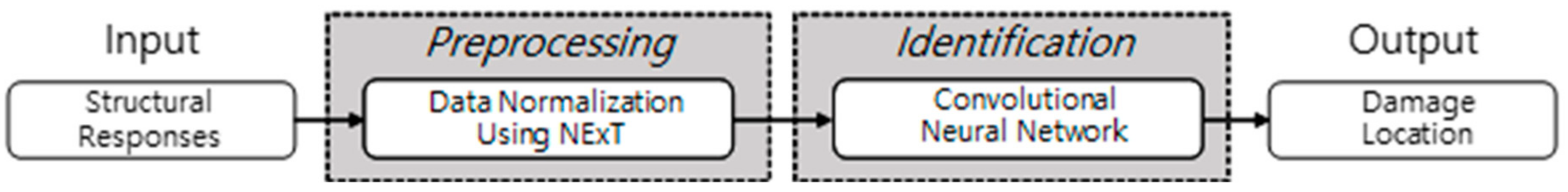
In this report, a time-series deep neural network is presented for automated structural damage detection using a data normalization technique and 1-D CNN. The data normalization technique converts raw measurements with any arbitrary length to a specified size of free vibration, preserving the excitation quality of the measurements, and the 1-D CNN detects and localizes damage on a structure.

For training and validation, the beam was excited with random and traffic loadings for 20 s, and the damage was simulated as 20%, 30%, and 50% of the single elemental stiffness loss. After training, the trained network was tested considering an untrained input size as well as a randomly several damage severities between 20 and 50%.

The remainder of this report is organized as follows. In Section 2, the proposed data normalization technique and CNN structure used are explained. In Section 3, datasets for training and validation are generated through numerical simulations conducted on a 10-element beam model, under 20%, 30%, and 50% of damage to a single random element on a beam. In this study, random and traffic loading excitations were used to validate the performance of the proposed network under nonstationary traffic loading to simulate the environment of ambient field vibration testing. In Section 4, the application of the proposed trained model to training datasets that have different measurement times and damage severities is described, and the accuracy of the proposed method is discussed. Finally, in Section 5, a summary and the conclusions drawn from the study are provided.

2. Proposed Method

A deep-neural-network-based approach is presented to detect structural damage from varying sizes of structural acceleration measurements. The proposed method has two components (see Figure 1): (a) Data normalization as preprocessing and (b) 1-D CNN for classifying the location of the structural damage.

2.1. Data Normalization through NExT

The natural excitation technique (NExT) [27] uses auto- and cross-correlation functions for two measurements of a structure to replace an impulse response for modal testing, enabling a structure to be tested in an ambient environment. The correlation between the two measurements is a superposition of decaying oscillations, which are characterized by the natural frequencies and damping ratios of the structure.

The correlation function R_ij(T) between two measurements at locations i and j in terms of time lag T is expressed as

$$R_{ij}(T)={\displaystyle \sum _{r=1}^N[\frac{{\varphi }_i^r{Q}_j^r}{m^r{\omega }_d^r}}\exp (-{\xi }^r{\omega }_n^{r}T)\sin ({\omega }_d^{r}T+{\theta }_r)]$$

(1)

where the superscript r denotes a particular mode from a total of N modes, ${\varphi }_i^r$ is the mode shape at location i at the r-th mode, $m^r$ is the modal mass in r-th mode, $Q_j^r$ is constant associated with response at node j, ${\omega }_n^r$ is the r-th natural frequency, ${\xi }^r$ is the r-th modal damping ratio, and ${\theta }_r$ is the phase angle associated with the r-th modal response.

In this study, the correlation functions for all sensor locations were obtained by inverse Fourier transform of cross power spectral density (CPSD) between two measurements at i and j as

$$R_{ij}={\Im }^{-1}\{S_{ij}\},\hspace{0.17em}R=\left[\begin{array}{cccc}{R}_{11}& R_{12}& \cdots & R_{1m}\\ R_{21}& R_{22}& \cdots & R_{2m}\\ ⋮& ⋮& \ddots & ⋮\\ R_{m1}& R_{m2}& \cdots & R_{mm}\end{array}\right]\in {\Re }^{m\times m\times \raisebox{1ex}{$n$}\!\left/ \!\raisebox{-1ex}{$2$}\right.}$$

(2)

where S_ij is the CPSD between measurements at i and j, m is the number of sensors, and n is the number of discrete Fourier transforms. The correlation functions in Equation (2) are used as the input data for a 1-D CNN. The proposed data normalization can accept measurements with different data sizes and sampling rates and normalize them to the same data size for flexible deep neural network applications. In the input layer, the normalized correlation functions are reshaped to $m^2\times \raisebox{1ex}{$n$}\!\left/ \!\raisebox{-1ex}{$2$}\right.$ for training the proposed deep neural network. For example, if nine accelerations are measured and the number of discrete Fourier transforms is 2048, the size of the normalized cross-correlation is 81 × 1024 for nine acceleration measurements on a beam, regardless of the number of samples for the measurement. The normalized input is fed into the 1-D CNN that is introduced in the following section.

2.2. Convolutional Neural Network

A CNN [28] is proposed to extract features automatically from time-series measurements and detect damage locations, as shown in Figure 2. The m-channel acceleration measurements are normalized and reshaped to $m^2\times \raisebox{1ex}{$n$}\!\left/ \!\raisebox{-1ex}{$2$}\right.$ and used as an input layer using Equation (2), where n is the number of discrete Fourier transforms. Following the input layer, three 1-D convolutional layers followed by batch normalization [29] and rectified linear unit (ReLU) [30] are used as a baseline architecture. Global average pooling (GAP) [31] and fully connected layers are used for the damage localization task. The features of the input layer are extracted through the convolutional layer and aggregated by GAP, and the damage location is classified by the fully connected layer. In addition, nonlinearity was added to the model through the ReLU activation function, and the input of each layer was normalized through batch normalization. The details of convolutional neural network architecture is described in

Table 2. Detail of architecture layers.

Layer	Input	Output	Feature	Kernel	Stride	Padding	Activation	Batch Normalization
Input	1024, 81	-	-	-	-	-	-	-
Conv.	1024, 81	1024, 128	128	8	1	Same	ReLU	True
Conv.	1024, 128	1024, 128	128	5	1	Same	ReLU	True
Conv.	1024, 128	1024, 128	128	3	1	Same	ReLU	True
GAP	1024, 128	128	-	-	-	-	-	-
Dense	128	11	-	-	-	-	Softmax	-
Output	11	-	-	-	-	-	-	-

.

2.3. One-Dimensional Convolution Layer

Convolution is an operator that multiplies one function by inverted values of another function and then aggregates it against the interval to obtain a new function. CNN creates a circuit of the input data at specified intervals, synthesizes it by channel, and makes the sum of the composite product of all channels into feature map H.

$$H_i=H_{i-1}\otimes W_i^C+b_i^C$$

(3)

where i indicates the number of layers in the network, and the ⊗ symbol indicates a convolution operation. The 1-D convolutional layer performs element-by-element multiplication of the input array and the kernel along the temporal axis of the input array. One-dimensional convolution consists of simple array operations in forward propagation and backpropagation such that the computational complexity is lower than that of 2-D convolution. The raw 1-D data are processed and learned to extract features that are used in the classification task.

2.4. Batch Normalization

The deep-learning model is a gradual way to learn meaningful expressions in a series of deep layers. This means learning to express features in a continuous layer. As the layer deepens, learning instability, such as gradient vanishing/gradient exploding, can occur while performing backpropagation operations. Batch normalization is a method that prevents “internal covariance shift,” a phenomenon in which the distribution of inputs varies on each floor or each activation function, by conducting normalization in minibatch units. The average and standard deviations for each feature are obtained and then normalized, and a new value is created using the scale factor and shift factor.

$${\widehat{x}}_i=\frac{x_i-{\mu }_B}{\sqrt{{\sigma }_B^2+\epsilon }}$$

(4)

$$y_i=\gamma {\widehat{x}}_i+\beta \equiv B{N}_{\gamma ,\beta }\left(x_i\right)$$

(5)

where ${\mu }_B$ denotes the average of minibatch B, and ${\sigma }_B$ is the standard deviation of minibatch B. The parameters $\gamma$ and $\beta$ are learned through backpropagation that adjusts the normalized values to avoid being driven to zero. The parameter $\epsilon$ is an extremely small constant to prevent the denominator from becoming zero.

2.5. Rectified Linear Unit (ReLU)

An activation function outputs a signal by entering it and processing it properly. Several types of activation functions exist, and the decision about the activation function considerably affects the results. The activation function is used to add nonlinearity to the output value of the convolutional layer, such as sigmoid, tanh, and ReLU.

$$f\left(x\right)=\max \left(0,x\right)$$

(6)

ReLU is the most commonly used nonlinear activation function in CNNs. Because ReLU is a nonsaturated function, and the gradient is zero if the input values are less than zero, and learning occurs if the input is greater than one. In addition, faster calculations and convergence rates can be achieved using ReLU.

2.6. Global Average Pooling

The pooling layer is used to reduce the size of the activation map or to emphasize specific features by receiving output data from the convolution layer as input. The pooling operation works by collecting the maximum value of a specific area or by averaging the values obtained for a specific area. In this study, the model uses GAP, in which window size or stride does not need to be designated; thus, overfitting is avoided. Unlike average pooling, which extracts only the average from a specific area and applies it after every convolutional layer, GAP derives the mean of the node values for each feature map. The GAP layer performs dimensionality reduction where the input is $h\times w\times d$ and is reduced to $1\times 1\times d$ by taking the average of all $hw$ values (see Figure 3). The 1-D GAP block takes a 2-D tensor ($data points\times channels$) and computes the average of all values ($data points$) for each of the channels.

2.7. Fully Connected Layer

After extracting the features including spatial information through the CNN, the extracted feature map is classified through the fully connected layer. A fully connected layer is the same operation as a general neural network, and the input is a 1-D array.

$$H_i=flatten\left(H_{i-1}\right)\times W_i^f+b_i^f$$

(7)

For multilabel classification, softmax is mainly used; the softmax function is also a type of activation function. If sigmoid or tanh are mainly used for binary classification, softmax is used for multilabel classification. Softmax in Equation (8) is a function that normalizes all the input values from 0 to 1. The class with the largest output value among the outputs generated by the probability is considered.

$$y_i=\frac{e^{x_i}}{{{\displaystyle \sum }}_{k=1}^K{e}^{x_k}}$$

(8)

3. Numerical Validation

3.1. Simulation Model

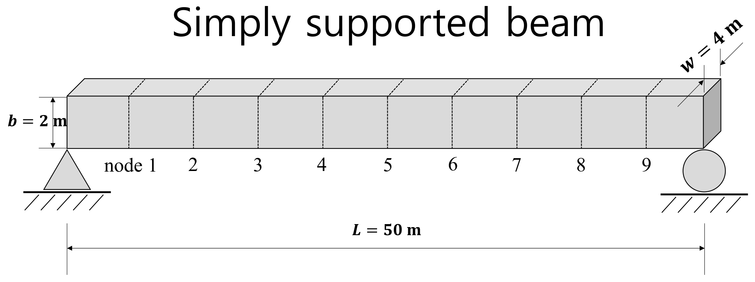
Numerical simulations were conducted to generate a database for the proposed automated structural damage detection method. A simply supported beam with a length of 50 m was modeled with a 10-element Bernoulli beam (see Figure 4). The cross section of the model was 4 × 2 m (width × height), the modulus of elasticity was 210 GPa, the density was 7850 $\mathrm{kg}/{\mathrm{m}}^3$, and the damping ratio was 2%. The three major natural frequencies of the beam without damage were 1.85, 7.52, and 16.8 Hz. Damage was simulated by reducing the flexural rigidity of the damaged element by 20%, 30%, and 50%.

To excite the structure with different loading cases, two loading conditions—random excitation and traffic loading excitation—were considered. A random excitation was provided to validate the proposed method in an ideal condition where all frequency spectra are excited so as to obtain precise modal parameters. Traffic loading was considered for the actual excitation of a structure, which requires sufficient measurement time for accurate modal analysis.

Random excitation was modeled with a normal distribution with a mean of 0 and a standard deviation of 20 kN at a single node randomly on the beam for each simulation case. Traffic loading was modeled as a three-wheel truck moving on the beam at different speeds from left to right (nodes 1 to 9). The force on the three wheels weighed 35 kN with 10% random force on the front and 145 kN with 10% random force added to two rear axles. The distance between the front and rear axles was 4.3 m, and that of the two rear axles was 9.0 m.

Sensor noise was assumed to be white Gaussian noise with a noise density of $100 \mathsf{\mu }\mathrm{g}/\sqrt{\mathrm{Hz}}$. The sampling rate was determined to be 100 Hz, and responses were generated using MATLAB Simulink with the ODE8 solver.

3.2. Data Generation for Training

For training of the proposed model, 24,000 datasets were generated with 50% random excitation and 50% traffic loading excitation, 20,000 datasets were generated for training, and 4000 datasets were used for validation. Two training cases were conducted to figure out the effect of data normalization pre-processing step (see

Table 3. Configurations of training cases.

	Case 1		Case 2
	Random Excitation	Traffic Loading	Random Excitation	Traffic Loading
Sampling Time (s)	60	60	20–60	20–60
Damage Severity (%)	0/20/30/50	0/20/30/50	0/20/30/50	0/20/30/50
Velocity (km/h)		30/40/50	-	30/40/50
No. of Vehicles		8~10	-	random

). The first case consisted of datasets with sampling time of 60 s while varying sampling times from 20 to 60 s were applied to the second case. Each case includes random excitation and traffic loading datasets. Note that 20 to 60 s data was created by randomly truncating 60 s data. These two cases were compared to find out how long data length, i.e., beam excitation, affects the learning outcome and how data normalizing affects. To label the location of damage, 11 categories were prepared. Label 0 indicates an intact condition, whereas labels 1 to 10 indicate a single damage location that corresponds to the element number. Because there were 10 labels for damage (i.e., elements 1 to 10) and one label for the intact condition, the number of intact datasets was increased so that the number of intact datasets was equal to the number of damage datasets to handle data unbalancing [32,33,34,35].

Figure 5 shows the random excitation and resulting acceleration response measured at node 1. To simulate traffic loading, three to five AASHTO trucks were designed to pass the beam randomly with velocities of 30, 40, and 50 km/h, as summarized in Table 3. Trucks are set to depart randomly so that various acceleration amplitudes can be generated (see Figure 6).

The simulated acceleration measurements were normalized by NExT to an input layer of 81 × 1024 and fed into a 1-D CNN.

3.3. Training and Validation

The simulated acceleration measurements were trained with the proposed deep network for automated damage localization. The nine-channel accelerations were normalized using NExT and then standardized to have a mean of 0 and a standard deviation of 1. The preprocessed input data were fed to a series of 1-D convolution layers that have 128 filters with kernel sizes of 8, 5, and 3. For better convergence, the kernels were initialized by the uniform He initialization scheme proposed by He et al. 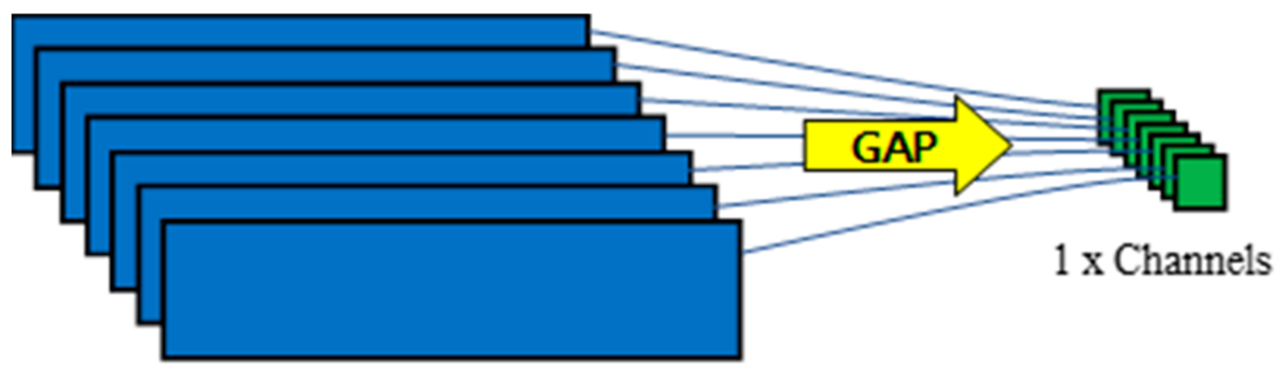[36], which samples from the uniform distribution. To avoid the overfitting issue, a batch normalization layer was added at the end of each 1-D convolution layer followed by GAP layers. The detailed configurations of training are summarized in

Table 4. Training case of random excitation.

Name	Value	Description
Batch size	128	Size of data used in training step
Steps per epoch	8	Number of steps per epoch
Total epochs	1000	Number of training epochs
Initial learning rate	$1\times {10}^{-5}$	Initial learning rate of Adam optimizer
${\beta }_1$	0.9	Parameter of Adam optimizer, weight of the momentum term
${\beta }_2$	0.999	Parameter of Adam optimizer, controlling the decay of learning rate
Epsilon	$1\times {10}^{-7}$	Parameter of Adam optimizer, constant for numerical stability

. Intel i9-9900x and Nvidia RTX2080Ti were used for training datasets, and a single training epoch cost 12 s.

3.4. Training Results and Discussion

For demonstration of training results, classification accuracy of each validation datasets is shown in

Table 5. Classification results of training cases.

	Case 1: 60 s of Data		Case 2: 20–60 s of Data
	Random Excitation	Traffic Loading	Random Excitation	Traffic Loading
Validation accuracy (%)	99.90	99.20	99.30	97.20

. According to classification results, Case 1 shows better classification capability in both cases. These results can lead us to the fact that training with longer data, which represents higher degree of excitation can provide more information to train the model. However, the longer the data, the longer the model takes to learn and harder to use for real world applications. For example, training a 60-s-long raw data with an input size of 9 × 6000 takes 34 s per epoch, whereas normalized 81 × 1024 takes 13 s. Thus, to secure learning efficiency in time-series deep learning model for structural damage detection, the proposed data normalization step is essential.

A comparison was made between the proposed method and the model proposed by Lin et al. [10]. Since the existing model was originally proposed to train with raw acceleration data, 10.24 s of raw acceleration data of which the size is 9 × 1024 was used for training. Furthermore, for demonstration of proposed data normalization, Case 1 dataset was used with the existing model.

As shown in

Table 6. Performance comparison of proposed model.

Network Architecture	Validation Accuracy on Different Loading Cases (%)
	Random Excitation	Traffic Loading
Proposed model (Data Normalization + CNN)	99.90	99.20
Lin et al. [10] (CNN)	81.20	59.80
Lin et al. [10] (Data Normalization + CNN)	97.30	89.60

, classification accuracy is 99.90% and 81.20% under random excitation for the proposed method and the existing model, respectively. The proposed method showed 18.70% better performance in damage classification compared to existing model. It is noteworthy that the accuracy of the models using traffic loading clearly show excellence of the proposed model. The proposed method showed 99.20% of accuracy while the existing model exhibited 59.80% of classification accuracy. The difference is resulted from the use of the proposed data normalization that allows to aggregate frequency-domain information compared to instant time-domain information presented in the existing model.

As a result of applying the data normalization method to existing model, the classification accuracy was significantly improved. However, in the existing model, the accuracy in the training process reached 100% at 98th epoch, but the validation accuracy did not exceed 93%. Since the existing model used max-pooling layers after convolutional layers, the overfitting issue was presented. On the other hand, GAP layer added to the proposed method instead of max-pooling layers addressed overfitting issue of the exiting model yielding better performance.

4. Application to New Datasets

4.1. Dataset for Application Test

One thousand datasets for random excitation and traffic loading were generated to evaluate the proposed model for new datasets that were different from the trained dataset in that sampling time was extended from 60 to 120 to 150 s, and damage severity was randomly selected to be 0% and 20–50%. Additionally, the number and velocity of vehicles were increased.

Table 7. Configurations of application datasets.

Load	Parameters	Training Dataset	Application Dataset
Random Excitation	Sampling Time (s)	60	120–150
	Damage Severity (%)	0/20/30/50	0/20–50
Traffic Loading	Sampling Time (s)	60	120–150
	Damage Severity (%)	0/20/30/50	0/20–50
	Velocity (km/h)	30/40/50	60/70/80/90/100
	No. of Vehicles	8–10	15–20

compares the trained dataset and the new dataset for validation.

4.2. Results and Discussion

The test results for each category that indicate the damage location are given in

Table 8. Classification result of application datasets under random excitation.

		Predicted Damage Location
		0	1	2	3	4	5	6	7	8	9	10	Total	Accuracy (%)
Actual damage location	0	88											88	100
	1		101										101	100
	2			107									107	100
	3				92								92	100
	4					83							83	100
	5						93						93	100
	6							94					94	100
	7								108				108	100
	8									89			89	100
	9										68		68	100
	10											77	77	100
	Total	88	101	107	92	83	93	94	108	89	68	77	1000	100

and

Table 9. Classification result of application datasets under traffic loading excitation.

		Predicted Damage Location
		0	1	2	3	4	5	6	7	8	9	10	Total	Accuracy (%)
Actual damage location	0	81											81	100
	1	1	77										78	98.72
	2		1	93									94	98.94
	3				84								84	100
	4					123							123	100
	5	1					97		1				99	97.98
	6	2						83					85	97.65
	7								98				98	100
	8	1								76			77	98.70
	9										93		93	100
	10	1									2	85	88	96.59
	Total	87	78	93	84	123	97	83	99	76	95	85	1000	99.00

for random excitation and traffic loading, respectively.

According to the test results shown in Table 8 and Table 9, the classification accuracy for random excitation was perfect and 1.0% higher than for traffic loading. Most of the misclassifications occurred in determining the existence of damage in the traffic loading case, whereas the random excitation case shows perfect classification result. These results demonstrate that the system vibrates more when random excitation is used than when traffic loading is used; thus, random excitation is used for assessing the status. However, considering the application to real structures that are tested with ambient vibration, the test result of traffic loading shows the robustness of the proposed method with a high accuracy of 99.00%.

Table 10. Confusion matrix of random excitation.

		Actual
		Intact	Damaged
Predicted	Intact	TP (88)	FP (0)
	Damaged	FN (0)	TN (912)

and

Table 11. Confusion matrix of traffic loading.

		Actual
		Intact	Damaged
Predicted	Intact	TP (81)	FP (6)
	Damaged	FN (0)	TN (913)

summarize the confusion matrix of each case that represents the classification capability of whether the system is intact or damaged. For analysis, “intact” is considered positive and “damage” is considered negative. From the confusion matrix, recall and fallout, represented by the true positive rate (TPR) and false positive rate (FPR), respectively, can be analyzed. TPR represents the ratio of the number predicted as positive cases to the number of actual positive cases and can be expressed

$$TPR= \frac{TP}{TP+FN}$$

(9)

FPR represents the ratio of those predicted as positive cases to the number of actual negative cases and is expressed as

$$FPR= \frac{FP}{TN+FP}$$

(10)

In both random excitation and traffic loading cases, the trained model showed that the TPR was 100% and had excellent capability to categorize “intact.” On the other hand, the capability to categorize damage represented by FPR was 0% for random excitation and 0.65% for traffic loading. These results show that the trained model performs well for classification of whether the condition of the structure is intact or damaged.

To show the performance of trained model, visualization using t-distributed stochastic neighbor embedding (t-SNE) [37] was conducted. The t-SNE is a nonlinear dimensionality reduction technique used to visualize high-dimensional data in low-dimensional space. This technique was used to create 2-D distribution map of the predicted location of damage and intact with the output from GAP layer, which was right before the classification layer.

Two 2-D maps, random and traffic loading, are shown in Figure 7, and each map shows 1000 points from test datasets. Figure 7 shows that points in the same category are close to each other and form clusters. Clustering was observed more clearly for random excitation result than for traffic loading.

5. Conclusions

An automated damage detection method using a deep neural network was presented. The proposed method for automated structural damage detection comprises two main contributions. (1) Data normalization is performed using NExT to compress and normalize the input data length. The acquired data can vary according to the measurement environment and purpose. Normalizing and quantifying the data length are critical to damage detection through deep neural networks because deep neural networks only work for trained data lengths. (2) A CNN is used to localize damaged elements. The proposed convolutional network can localize damaged elements from normalized input acceleration signals without any damage-sensitive extraction process.

A numerical model of a simply supported beam was excited by random ambient load and traffic loading, and acceleration responses were extracted from nine nodes. Sensor noise is considered to demonstrate the reality of the measurement. Noisy acceleration signals from nine nodes were correlated with each other to normalize and quantify the data length, and a fully correlated response matrix was generated. The fully correlated response matrix is the input of the deep neural network, and the output is the location of the damaged element.

For the training of the proposed method, datasets were generated using random excitation and traffic loading, and single damage was randomly applied to one of the elements. A total of 20,000 datasets for training (10,000 for each load) and 4000 datasets for validation (2000 for each load) were used to train the model. The number of intact data (i.e., category 0) was greater than each damage data (from category 1 to category 10) to balance the number of intact to total number of damage data. For representation of effect of data normalization, two training cases were compared. The resulting classification accuracy for Case 1 was 99.90% and 99.20% for random excitation and traffic loading datasets, respectively. Through the results, it was found that by using data normalization technique in the pre-processing step, longer data can be used for training to enhance classification capability of trained model.

The proposed method was validated through tests with different conditions for generating datasets. For random excitation, the sampling time was increased. For traffic loading, the velocity, number of trucks, and sampling time were increased. In addition, 0% or 20–50% of damage was chosen at random for both loads. The classification accuracy of random excitation was 100% and that of traffic loading was 99.00%.

Future work is planned to focus on problems caused by the low severity of damage. The proposed method using different deep neural networks rather than 1-D CNN will be studied to improve classification accuracy. Furthermore, to enhance the effectiveness of the proposed method, the classification of multiple damages and prediction of damage severity will be studied.

References

1. Casas, J.R.; Moughty, J.J. Bridge damage detection based on vibration data: Past and new developments. JFiBE 2017, 3, 4. [Google Scholar] [CrossRef] [Green Version]
2. Doebling, S.W.; Farrar, C.R.; Prime, M.B.; Shevitz, D.W. Damage Identification and Health Monitoring of Structural and Mechanical Systems from Changes in Their Vibration Characteristics: A Literature Review; Los Alamos National Lab.: Los Alamos, NM, USA, 1996. [Google Scholar]
3. Sohn, H.; Farrar, C.R.; Hemez, F.M.; Czarnecki, J.J. A Review of Structural Health Review of Structural Health Monitoring Literature 1996–2001; Los Alamos National Laboratory: Los Alamos, NM, USA, 2002. [Google Scholar]
4. Fan, W.; Qiao, P.J.S.H.M. Vibration-based damage identification methods: A review and comparative study. J. Civil Struct. Health Monit. 2011, 10, 83–111. [Google Scholar] [CrossRef]
5. Carden, E.P.; Fanning, P. Vibration based condition monitoring: A review. Struct. Health Monit. 2004, 3, 355–377. [Google Scholar] [CrossRef]
6. Das, S.; Saha, P.; Patro, S.K. Vibration-based damage detection techniques used for health monitoring of structures: A review. J. Civil Struct. Health Monit. 2016, 6, 477–507. [Google Scholar] [CrossRef]
7. Gomes, G.F.; Mendez, Y.A.D.; da Silva Lopes Alexandrino, P.; da Cunha, S.S., Jr.; Ancelotti, A.C., Jr. A review of vibration based inverse methods for damage detection and identification in mechanical structures using optimization algorithms and ANN. Arch. Computat. Methods Eng. 2019, 26, 883–897. [Google Scholar] [CrossRef]
8. Yan, Y.; Cheng, L.; Wu, Z.; Yam, L.M. Development in vibration-based structural damage detection technique. Mech. Syst. Signal Process. 2007, 21, 2198–2211. [Google Scholar] [CrossRef]
9. Wang, L.; Chan, T.H. Review of vibration-based damage detection and condition assessment of bridge structures using structural health monitoring. In Proceedings of the Second Infrastructure Theme Postgraduate Conference: Rethinking Sustainable Development-Planning, Infrastructure Engineering, Design and Managing Urban Infrastructure; Queensland University of Technology: Brisbane City, Australia, 2009. [Google Scholar]
10. Lin, Y.Z.; Nie, Z.H.; Ma, H.W. Structural damage detection with automatic feature-extraction through deep learning. Comput. Aided Civil Infrastruct. Eng. 2017, 32, 1025–1046. [Google Scholar] [CrossRef]
11. Zhang, Y.; Miyamori, Y.; Mikami, S.; Saito, T. Vibration-based structural state identification by a 1-dimensional convolutional neural network. Comput. Civ. Infrastruct. Eng. 2019, 34, 822–839. [Google Scholar] [CrossRef]
12. Lee, K.; Jeong, S.; Sim, S.-H.; Shin, D.H. A Novelty Detection Approach for Tendons of Prestressed Concrete Bridges Based on a Convolutional Autoencoder and Acceleration Data. Sensors 2019, 19, 1633. [Google Scholar] [CrossRef] [Green Version]
13. Khodabandehlou, H.; Pekcan, G.; Fadali, M.S. Vibration-based structural condition assessment using convolution neural networks. Struct. Control Health Monit. 2019, 26, e2308. [Google Scholar] [CrossRef]
14. Guo, T.; Wu, L.; Wang, C.; Xu, Z. Damage detection in a novel deep-learning framework: A robust method for feature extraction. Struct. Health Monit. 2020, 19, 424–442. [Google Scholar] [CrossRef]
15. Pathirage, C.S.N.; Li, J.; Li, L.; Hao, H.; Liu, W.; Wang, R. Development and application of a deep learning–based sparse autoencoder framework for structural damage identification. Struct. Health Monit. 2019, 18, 103–122. [Google Scholar] [CrossRef] [Green Version]
16. Abdeljaber, O.; Avci, O.; Kiranyaz, S.; Gabbouj, M.; Inman, D.J. Real-time vibration-based structural damage detection using one-dimensional convolutional neural networks. J. Sound Vib. 2017, 388, 154–170. [Google Scholar] [CrossRef]
17. Avci, O.; Abdeljaber, O.; Kiranyaz, S.; Hussein, M.; Inman, D.J. Wireless and real-time structural damage detection: A novel decentralized method for wireless sensor networks. J. Sound Vib. 2018, 424, 158–172. [Google Scholar] [CrossRef]
18. Abdeljaber, O.; Avci, O.; Kiranyaz, M.S.; Boashash, B.; Sodano, H.; Inman, D.J. 1-D CNNs for structural damage detection: Verification on a structural health monitoring benchmark data. Neurocomputing 2018, 275, 1308–1317. [Google Scholar] [CrossRef]
19. Rafiei, M.H.; Adeli, H. A novel unsupervised deep learning model for global and local health condition assessment of structures. Eng. Struct. 2018, 156, 598–607. [Google Scholar] [CrossRef]
20. Hung, D.V.; Hung, H.M.; Anh, P.H.; Thang, N.T. Structural damage detection using hybrid deep learning algorithm. J. Sci. Technol. Civil Eng. 2020, 14, 53–64. [Google Scholar] [CrossRef] [Green Version]
21. Teng, S.; Chen, G.; Gong, P.; Liu, G.; Cui, F. Structural damage detection using convolutional neural networks combining strain energy and dynamic response. Meccanica 2019. [Google Scholar] [CrossRef]
22. Gulgec, N.S.; Takáč, M.; Pakzad, S.N. Convolutional neural network approach for robust structural damage detection and localization. J. Comput. Civ. Eng. 2019, 33, 04019005. [Google Scholar] [CrossRef]
23. Azimi, M.; Pekcan, G. Structural health monitoring using extremely compressed data through deep learning. Comput. Civ. Infrastruct. Eng. 2020, 35, 597–614. [Google Scholar] [CrossRef]
24. Fang, X.; Luo, H.; Tang, J. Structural damage detection using neural network with learning rate improvement. Comput. Struct. 2005, 83, 2150–2161. [Google Scholar] [CrossRef]
25. Sajedi, S.O.; Liang, X. Vibration-based semantic damage segmentation for large-scale structural health monitoring. Comput. Aided Civil Infrastruct. Eng. 2020, 35, 579–596. [Google Scholar] [CrossRef]
26. Zhang, G.; Tang, L.; Liu, Z.; Zhou, L.; Liu, Y.; Jiang, Z. Machine-learning-based damage identification methods with features derived from moving principal component analysis. Mech. Adv. Mater. Struct. 2020, 27, 1789–1802. [Google Scholar] [CrossRef]
27. James, G.; Carne, T.G.; Lauffer, J.P. The Natural Excitation Technique (NExT) for Modal Parameter Extraction from Operating Structures. Modal Anal. 1995, 10, 260. [Google Scholar]
28. LeCun, Y.; Haffner, P.; Bottou, L.; Bengio, Y. Object recognition with gradient-based learning. In Shape, Contour and Grouping in Computer Vision; Springer: Berlin/Heidelberg, Germany, 1999; pp. 319–345. [Google Scholar]
29. Ioffe, S.; Szegedy, C. Batch normalization: Accelerating deep network training by reducing internal covariate shift. arXiv 2015, arXiv:1502.03167. [Google Scholar]
30. Nair, V.; Hinton, G.E. Rectified linear units improve restricted boltzmann machines. In Proceedings of the 27th international conference on machine learning (ICML-10), Haifa, Israel, 21–24 June 2010; pp. 807–814. [Google Scholar]
31. Lin, M.; Chen, Q.; Yan, S. Network in network. arXiv 2013, arXiv:1312.4400. [Google Scholar]
32. Mazurowski, M.A.; Habas, P.A.; Zurada, J.M.; Lo, J.Y.; Baker, J.A.; Tourassi, G.D. Training neural network classifiers for medical decision making: The effects of imbalanced datasets on classification performance. Neural. Netw. 2008, 21, 427–436. [Google Scholar] [CrossRef] [Green Version]
33. Japkowicz, N. Learning from imbalanced data sets: A comparison of various strategies. In Proceedings of AAAI Workshop on Learning from Imbalanced Data Sets; The AAAI Press: Menlo Park, CA, USA, 2000; pp. 10–15. [Google Scholar]
34. Maloof, M.A. Learning when data sets are imbalanced and when costs are unequal and unknown. In Proceedings of ICML-2003 Workshop on Learning from Imbalanced Data Sets II; CML: Washington, DC, USA, 2003. [Google Scholar]
35. Elazmeh, W.; Japkowicz, N.; Matwin, S. Evaluating misclassifications in imbalanced data. In Proceedings of the European Conference on Machine Learning, Ghent, Belgium, 14–18 September 2020; pp. 126–137. [Google Scholar]
36. He, K.; Zhang, X.; Ren, S.; Sun, J. Delving deep into rectifiers: Surpassing human-level performance on imagenet classification. In Proceedings of the IEEE International Conference on Computer Vision, Santiago, Chile, 7–13 December 2015; pp. 1026–1034. [Google Scholar]
37. Van der Maaten, L.; Hinton, G. Visualizing data using t-SNE. J. Mach. Learn. Res. 2008, 9, 2579–2605. [Google Scholar]
Figure 1. Proposed damage identification method.
Applsci 11 02610 g001
Figure 2. One-dimensional convolutional neural network architecture.
Applsci 11 02610 g002
Figure 3. Global average pooling (GAP) layer.
Applsci 11 02610 g003
Figure 4. Simply supported beam for numerical validation.
Applsci 11 02610 g004
Figure 5. Examples of random excitation—(a) load on node 1 and (b) acceleration response of node 1.
Applsci 11 02610 g005
Figure 6. Examples of traffic loading excitation—(a) load on node 1 and (b) acceleration response of node 1.
Applsci 11 02610 g006
Figure 7. t-distributed stochastic neighbor embedding (t-SNE) visualization of untrained new datasets with measurement size (e.g., 120–150 s) and damage severity (intact and random damage quantity of 20–50%): (a) Random excitation and (b) traffic loading.
Applsci 11 02610 g007