A Numerical Investigation of Laser Beam Welding of Stainless Steel Sheets with a Gap

Abstract

Keyhole laser beam welding (LBW) of 304L stainless steel sheets with a gap in between was numerically simulated with a three-dimensional, transient, multi-physical model for laser material processing based on the finite volume method (FVM). First, the model’s ability to reproduce experimental results on a relatively coarse computational mesh within reasonable computing time, so as to serve as process optimization tool, is presented. An example of process optimization is shown, wherein a given set of weld seam quality criteria is fulfilled by iteratively optimizing a secondary laser beam. The relatively coarse mesh, in combination with a good model calibration for the experimental conditions, allows for sufficiently fast simulations to use this approach for optimization tasks. Finally, using a finer spatial and temporal discretization, the dynamic processes in the vicinity of the keyhole leading to the formation of pores are investigated. The physical phenomena predicted by the simulation are coherent with experimental observations found in literature.

1. Introduction

Keyhole laser beam welding (LBW) has gained importance in many industries—e.g., the automotive and aerospace industries—over the years. The advantages of LBW cover a high level of precision and speed, reduced distortion and a high potential for process automation [1]. It is difficult to experimentally investigate the many physical phenomena involved in laser beam welding, as post-experimental investigations do not provide sufficient information on process dynamics, and in-situ observations of the transient behavior, especially inside the keyhole, are not possible on all desired time and length scales. Zhang et al. [2] managed to directly observe the keyhole by employing a sandwich construction of stainless steel and a special type of glass, using a high-speed camera. However, such experiments require complex setups and do not allow for an investigation of real industrial specifications. Therefore, the development of models which are capable of accurately predicting the physical phenomena involved in LBW remains important and research is ongoing. Reliable models can then help gain understanding of the driving mechanisms behind the formation of defects such as lack of penetration, formation of humps, pores and end craters.

Models of different levels of complexity have been introduced in the past. Ki et al. [3] developed a model based on the level-set method for solving the multiphase flow problem, for which they employed some simplifications in the solution of the flow field. Ye and Chen [4] solved the Navier–Stokes equations for the fluid flow by assuming a fixed, cylindrical keyhole and a flat free surface of the liquid. Schöler et al. [5] developed a model for the calculation of the depth of a circular keyhole by exploiting characteristic time and length scales for laser beam welding processes. Noori Rahim Abadi et al. [6] recently used a volume-of-fluid approach within OpenFOAM to investigate the effect of beam shaping on the melt pool behavior in conduction mode laser beam welding. While their implementation was similar, in the model presented in Section 2.1 a crucial component needed for keyhole laser welding was added by implementing an evaporation model. Panwisawas et al. [7] developed a model for keyhole laser beam welding based on a volume-of-fluid approach by implementing it in OpenFOAM and also taking into account evaporation phenomena. A novel addition to the state of the art is provided by the model in Section 2.1 through the further distinction between two or more gaseous phases, which is of paramount importance when trying to gain a deeper understanding into the process of pore formation as described in Section 4. Furthermore, commercial software is available for the simulation of laser beam welding, e.g., that by Zhang et al. [8] for the simulation of keyhole laser beam welding. This, however, comes with the inconvenience of proprietary source code and the inability to change or add models. Apart from models concerned with the fluid dynamical description of LBW, a topic of great interest and practical relevance is the thermo-mechanical modeling of the process to gain insight in the formation of stresses. This is mostly done by the means of finite element methods, as was done by Liedl et al. [9] and was more recently investigated by Kik [10]. This topic is, however, not further discussed here, as the underlying method and approach are fundamentally different from what is presented here. Another issue of great practical importance in the field of LBW modeling is the prediction of the crystallographic microstructure of a weld bead, as its knowledge can help avoid problems such as solidification cracking. Such predictions have recently been made by Giudice and Sili [11] using an analytical model. The linking of a mechanistic microstructural growth model to the simulation model presented here is currently being realized [12].

An initial effort for developing a model capable of accurately simulating processes involved in laser-assisted manufacturing was made by Geiger et al. [13] and Otto et al. [14] by developing a universal multi-physical laser-material processing model based on the open source C++ toolbox OpenFOAM [15], using the volume-of-fluid method for solving the multiphase flow field. The model has since then been substantially improved at the Institute of Production Engineering and Photonic Technologies at Vienna University of Technology. The solver includes the Navier–Stokes equations and continuity equation, coupled with appropriate models for laser beam propagation, laser-material interaction, phase change, keyhole vapor pressure, surface tension and many more physical phenomena necessary to adequately simulate such complex processes. It is capable of accurately predicting a broad range of laser-assisted processes, including LBW, laser cutting, laser ablation using ultra-short laser pulses and many additive manufacturing processes (laser powder bed fusion, laser cladding, etc.) due to the most recent integration of the Lagrangian library into the solver [16,17].

In the automotive industry, welding of overlapping galvanized steel sheets is a common task, and thus much of the research on welding of sheets with the presence of a gap was done on this topic. As the boiling temperature of Zn lies well below the melting temperature of steel, the vaporization of Zn at the interface and its venting through the melt pool or keyhole can lead to the formation of various defects, including spatter, blowholes and lack of fusion. Several sophisticated techniques to overcome these problems have been suggested, e.g., cutting a slot along the to-be welded line, generating vent holes in the bottom sheet with a pulsed laser and producing humps on the interface surface. Additionally, many-pass strategies, and slow-speed welding, have been shown to mitigate the problem, but all of these techniques are irrelevant for the automotive industry because of increased processing time and complexity. By adding a suitable gap at the sheet interface, a stable process can be achieved, yielding high-quality weld seams [18,19,20]. On the flip side, the presence of a gap can cause different defects, including underfilling, porosity, “false friends” (misconnections without outside evidence), etc. These problems are inherent to gap welding and are independent from the previously described problem of Zn-evaporation and subsequent spatter formation. The reason for the occurrence of a gap in processes with stainless steel sheets that may not be galvanized is in part thermal deformation and the thereby introduced complexity of achieving perfect contact over the whole weld bead length by designing a reliable clamping system. These scenarios were the motivation behind the study presented here, and they study by Drobniak et al. [21]. In the case of the CUSTODIAN project, the presence of a gap was not added deliberately, but was a consequence of the geometry of the parts to be welded (e.g., segments of exhaust pipes pressed together), where a zero gap is not reasonable without a massive increase in processing accuracy to reach such tight tolerances. To better understand and prevent the formation of such defects, the simulation model presented here is used to investigate keyhole laser beam welding of stainless steel sheets with a gap.

Section 2.1 describes the simulation model used to perform the investigations presented here and points out further literature regarding the modeling approach. In Section 2.2, the calibration and validation of the model using results of laser beam welding experiments is presented and discussed. In Section 3, a methodology for process optimization through the use of the simulation model on a computationally inexpensive grid is presented. The process optimization was achieved through the addition of a secondary laser beam, which was iteratively adapted in simulations to achieve a set of quality requirements set for the weld and not previously achieved without the secondary beam. Some of the resulting welds are presented. In Section 4, the model is used on a finer computational grid to investigate the physical phenomena leading to pore formation in LBW of overlapping sheets with an interface gap. In Section 5, a conclusion is drawn and an outlook is provided.

2. Simulation Model

2.1. Description of the Model

The model is based on the open source C++ toolkit OpenFOAM [15], which provides a framework for using the finite-volume method to solve continuum mechanics problems described by partial differential equations. The solver is based on the OpenFOAM-native “multiphaseInterFOAM” solver, which itself is the n-phase extension of the well-known “interFoam” solver [22]. It uses the volume-of-fluid method to solve multiphase problems, involving an arbitrary number of different phases combined with the possibility of dynamic mesh refinement at run-time. This solver has been extensively modified and extended to make it suitable for the simulation of laser-material processing. An overview of the solver and incorporated models for other types of processes can be found in [17]. The models relevant for the simulation of laser beam welding are briefly explained in the following paragraph.

The propagation of laser beams of arbitrary shape (e.g., rings, rectangular, or elliptical) and intensity distribution (e.g., Gaussian, tophat, or Bessel) is calculated by solving a differential radiative transfer equation [23]. A ray tracing algorithm takes into account multiple reflections, which is crucial in keyhole welding simulations. Incident angle-dependent transmission and reflection are modeled according to Fresnel’s equations; absorption is calculated via Beer’s law. The state and temperature-dependent complex refractive index (consisting of the refractive index n and the extinction coefficient $\kappa$) of the material therefore needs to be known to correctly model the absorption of laser power within the material. This index is not only dependent on the material but also on the wavelength of the laser [24] and reliable information in the literature is scarce, especially for high temperature applications. Therefore, in many cases, both estimation and calibration of this parameter using experimental results are needed.

The amount of laser energy absorbed by the material, resulting from the propagation model described above, is included as a source term in the energy equation. The classical energy equation is split into one equation containing the conductive heat transfer and one transport equation for calculating the convective heat transport. Within each time step, the convective part of the energy equation is solved once the flow field is known. Then, the conductive part is solved, including the absorbed laser power as an additional source term. This approach is necessary because of the temperature-dependency of the material’s heat conductivity and capacity, which are needed within the conductive part of the energy equation.

Each material with its respective phases involved in the problem, i.e., solid, liquid and vapor, and ambient gas (e.g., surrounding air or shielding gas), is treated as a distinct phase in the multiphase solver. Phase changes are modeled as mass transfers between the respective phases via the Clapeyron equation and an accompanying energy transfer. The thus yielded phase change rates have an influence on the pressure, and therefore phase change and pressure have to be calculated together in an iterative manner.

The movement restriction of the solid material is realized through a porous bed model via Darcy’s law [25], where a source term in the momentum equation increases with the fraction of solid material inside a cell, letting the velocity approach zero for a solid phase far from any interface.

The solver is capable of dynamic mesh refinement to decrease computational costs. Initially a coarse hexahedral mesh is used, with the cells’ size being in the range of half the gap size. Then, dynamically throughout the simulation, the mesh is refined iteratively depending on the presence of propagating or absorbed laser power, presence of a liquid phase and presence of a re-solidified phase.

The initial (unrefined) computational grid was the same for all simulations presented within this work, except for the different gap widths. An isometric view of the entire computational domain is shown in Figure 1. The domain measured 30 mm × 8 mm × 5 mm, with the latter measurement being the height and varying slightly depending on the gap width. It was ensured that boundary conditions were not influencing the solution by performing test simulations on larger geometric domains. The initial grid shown in Figure 1 consists of 76,800 elements. The number of elements changed constantly during the course of each simulation due to the dynamic mesh refinement, reaching values of 250,000, depending on the specific simulation. Simulation S5, presented in Section 4, featured, due to the additional level of mesh refinement, approximately 50,000 additional elements. The refined mesh can be seen in Figure 2. The rise in computational times, however, mostly stems from the thus required smaller time step, as laid out in detail in Section 2.3.

2.2. Model Calibration and Validation

Before using the above-described model to simulate the process, some material properties, such as the complex refractive index and values for the surface energy of the material, need to be calibrated. Although some data on these properties are available in relevant literature, they are not material constants, but (at least) functions of alloy composition, impurities within the alloy, temperature and (in the case of the refractive index) laser wavelength. The dependency of surface tension on temperature is very sensitive to impurities in the form of surface-active elements, mainly oxygen and sulfur. Therefore, there are a lot of discrepancies in the available experimental measurements [26]. However, surface tension-related phenomena such as Marangoni currents are of great importance in weld pool dynamics [27], and therefore a fine-tuning of surface tension data against experimental results is necessary. In the case of the complex refractive index, this property and its temperature-dependence have a great influence on the laser-material interaction. Data are available for 304L stainless steel, e.g., in reference [28], but only one value is given for each melting and boiling temperature, respectively, with no information on temperature-dependency in between. Additionally, no information is provided as to which phases the values refer to, e.g., at the melting point, liquid or solid phase. As this property’s influence on the process is high, validation is necessary. Apart from the aforementioned material properties, discretization schemes used by the solver and the amount interface compression within the volume-of-fluid method need to be appropriately chosen in order to obtain a good fit regarding the experimental data. For this purpose, longitudinal and cross-sections of 304L stainless steel sheets welded under the presence of a gap were used. The welding experiments EX1–EX4 within this study were conducted at the facilities of AIMEN. The experimental setup consisted of an ABB IRB6600 robot carrying an Optoskand LBW tool which can provide a minimum spot diameter of 100 µm. The laser source was a Coherent fiber laser FL080 with a 100 µm diameter fiber, a wavelength of 1070 nm and a beam parameter product of 3.5 mm × mrad. No shielding gas was used. The experimental conditions are listed in

Table 1. Conditions of the laser beam welding (LBW) experiments EX1 and EX2 used for model calibration and validation.

Parameter	Unit	EX1	EX2
material	−	AISI304L	AISI304L
sheet thickness	mm	1	1
welding speed	mm/s	100	120
laser power	kW	3.5	4
laser wavelength	nm	1070	1070
laser M2	−	12.4	12.4
laser defocus	mm	7	7
laser radius on top sheet surface	mm	0.31	0.31
gap width	mm	0.3	0.4

.

The model was calibrated to reproduce the results of EX1 (Table 1). Another experiment, EX2, was then used to validate the model, to ensure the prevention of overfitting to the calibration conditions. In EX2, the gap width, welding speed and laser power were different from those in EX1. To validate the values for the complex refractive index, the simulation should be able to reproduce the penetration depth measured from the experiments and general heat input estimated from the volume of material molten during the experiments. To calibrate values for the surface energy of the materials, the shape of the cross-sections gained from the experiments should be matched, especially at the weld bead top and at the interface, where capillary forces play an important role. As a starting point, values for the liquid phase from Sahoo et al. [29] were taken and iteratively calibrated to fit the experimental data. The surface energy values for the solid phase were kept at a constant value, due to unavailability of concrete values for most metals. The final values for surface energy as a function of temperature and phase are plotted in Figure 3.

Figure 4 and Figure 5 show the comparison of experimental longitudinal and cross-sections of EX1 and EX2 and the corresponding simulations S1 and S2 (using the fully calibrated model), respectively. Both the penetration depth over most of the longitudinal section and the cross-sectional weld bead shape are in qualitative and reasonable quantitative agreement. Notably, the defect at the end of the weld bead in EX2 (right end of top longitudinal section in Figure 5), which resembles an end crater, because of the lack of material, resulting in an unfilled keyhole, was reproduced in simulation S2. In S2 (Figure 5), the plates were still joined, but the defect was clearly visible in terms of a decrease in weld bead height. A similar defect was—to a much smaller extent—also visible in EX1 (Figure 4).

2.3. Discussion on Mesh Density

In general, the mesh used for the spatial discretization of the computational domain should be dense enough, i.e., the cell size sufficiently small, to reach a mesh-independent solution. The temporal discretization during the solution procedure is determined by the Courant–Friedrichs–Lewy number, CFL, which is defined as [30]

$$CFL=\frac{u\Delta t}{\Delta x},$$

(1)

where u is the maximum velocity, $\Delta t$ denotes the time step and $\Delta x$ denotes the smallest cell length. By choosing $\Delta t$ in such a way that $CFL<1$, it is ensured that the fluid does not skip a computational cell during the advancement of one time step. It is then clear that a reduction in cell size by a factor of 2 does not only increase the number of cells by a factor 8 (due to three-dimensionality), but also leads to a forced increase in temporal resolution by a factor of 2 in the whole simulation domain. Therefore, a reduction in cell size has great influence on the computational cost of a simulation.

For the above-mentioned reasons, the model was carefully calibrated with the aim of reproducing experimental results in a timely manner so as to be able to use it for optimizing process parameters. During the optimization process, a great number of simulation runs had to be completed within a reasonable amount of time. Therefore, a mesh density was chosen that was sufficient for producing accurate results on a larger scale needed for gaining information about the weld bead shape, as this was the main criterion for the optimization process. It was noted that the cell size was not small enough to resolve many smaller scale effects, such as the dynamic waves formation occurring at the leading wall of the keyhole.

Within the scope of this paper, the simulation model was used to optimize results of LBW processes on the one hand (see Section 3), and to investigate highly dynamic small scale processes on the other hand (see Section 4). For the latter, the finite volume density was dynamically increased by a factor of 8 in the vicinity of the keyhole. This, however, increased the penetration depth and showed that it was underestimated by the coarser mesh.

One of the possible reasons for the increase in penetration when decreasing the cell size stems from the fact that the resolution of surface waves at the keyhole front slightly changes the local angle of incidence of the incoming laser beam, which has a great influence on absorption. The wave structures on the keyhole wall resolved by using a sufficiently fine computational grid, can be seen in Figure 6. It is clear that with increasing grid coarseness, smaller waves tend to be filtered out and only larger wave structures can be resolved.

The effect of laser energy absorption being sensitive to the local incident angle can be seen when plotting the absorption of laser radiation according to the Fresnel equations, which were also discussed by Beyer [24]

$$\begin{array}{cc}\hfill A_S& =1-\frac{a^2+b^2-2a·cos\alpha +{cos}^2\alpha }{a^2+b^2+2a·cos\alpha +{cos}^2\alpha },\hfill \end{array}$$

(2)

$$\begin{array}{cc}\hfill A_P& =1-\frac{a^2+b^2-2\left(a\left(n^2-{\kappa }^2\right)+2bn\kappa \right)cos\alpha +{\left(n^2+{\kappa }^2\right)}^2{cos}^2\alpha }{a^2+b^2+2\left(a\left(n^2-{\kappa }^2\right)+2bn\kappa \right)cos\alpha +{\left(n^2+{\kappa }^2\right)}^2{cos}^2\alpha },\hfill \end{array}$$

(3)

$$\begin{array}{cc}\hfill a^2& =\frac{1}{2}\left(\sqrt{\left(n^2-{\kappa }^2-{sin}^2\alpha \right)+4n^2{\kappa }^2}+n^2-{\kappa }^2-{sin}^2\alpha \right),\hfill \end{array}$$

(4)

$$\begin{array}{cc}\hfill b^2& =\frac{1}{2}\left(\sqrt{\left(n^2-{\kappa }^2-{sin}^2\alpha \right)+4n^2{\kappa }^2}-\left(n^2-{\kappa }^2-{sin}^2\alpha \right)\right),\hfill \end{array}$$

(5)

$$\begin{array}{cc}\hfill A& =\frac{A_S+A_P}{2},\hfill \end{array}$$

(6)

as a function of the angle of incidence, as can be seen in Figure 7. Here, the incident angle $\alpha$ is the angle between the laser beam direction and the surface normal; therefore, $\alpha ={90}^{\circ }$ corresponds to a laser beam parallel to the surface. $A_S$, $A_P$ and A denote absorption of radiation of perpendicular, parallel and no polarization, respectively. It is obvious that a small deviation in incident angle, especially in the regime of high incident angles, as is typical for keyhole welding, has a significant effect on the fraction of laser power absorbed by the material.

Another consequence of using smaller cells is the decrease in the energy required to reach the melting threshold inside a computational cell, since otherwise the same energy gets distributed over a larger volume. This effect also goes hand in hand with a decrease in numerical diffusion for more refined meshes.

The calibration using the coarser mesh thus yielded values for the complex refractive index (n and $\kappa$), and a minimum threshold for material in a cell to be taken into account for the absorption of laser energy and a maximum number of reflections being considered by the ray tracing algorithm, which compensated for the effects described above. When switching to a finer mesh, these parameters therefore would require a new calibration in order to produce results that are in agreement with the experiments. This was omitted due to the associated high computational cost, as the purpose of the simulations conducted using a finer mesh was not the reproduction of experiments or the use of data to adjust a real-world process, but the investigation of transient effects for the purpose of fundamental research.

3. Beam Shape Optimization

Using a sufficiently coarse mesh is a possibility for reducing computational costs and thus getting results faster, which is of paramount importance when applying any CFD model to a real-world application scenario and using it for optimizing many process parameters. To avoid unphysical results due to the coarseness of the mesh, careful calibration and validation have been performed (see Section 2.2). In the course of the CUSTODIAN project, a methodology was developed to increase the quality of a welded seam proposed by an industry partner. The quality requirements set for the welded seams are summarized in

Table 2. Weld quality requirements as defined by the industry partner.

Parameter	Value Range	Reference in Figure 8
total penetration	>50% of bead length	-
min. weld width at interface	>0.67 mm	(a)
lack of penetration	<0.2 mm	(b)
incompletely filled groove	<0.2 mm	(c)
excessive penetration	<0.4 mm	(d)
excess weld metal	<0.4 mm	(e)
undercut	<0.1 mm	(f)
root concavity	<0.2 mm	(g)

and schematically illustrated in Figure 8.

In this Section, an optimization approach is presented, where the addition of a secondary beam and its effect on the final weld bead geometry are studied. The advantages of a dual beam approach and the effect on material properties and quality criteria have been numerically investigated using commercial CFD software by Zhang et al. [31]. One advantage of using a secondary beam superimposed on the primary beam is the possibility of in-situ pre-heating or post-heating without the need for additional scans. The effects of laser based pre-heating and post-heating have previously been investigated by Saffer et al. [32].

The starting point was an elliptical beam that covered the whole of the melt pool with the aim of introducing more energy and thus fixing some of the issues. In the course of the project, this shape was changed to a rectangle due to its easier technical feasibility within the chosen beam shaping approach. Different energy distributions, sizes (length and width of rectangle) and positions relative to the primary beam (offset) have been tested using the simulation model to iteratively find the optimal beam shape for each experimental condition. At first, the influences of the parameters on the weld seam were investigated by testing some extreme values of each relevant parameter. The insights thus gained were used to iteratively tune the secondary beam parameters to fulfill all quality criteria listed in Table 2. The final improvements were reached through the use of a secondary beam with the aforementioned rectangular shape with varying parameters for width, length and power density, depending on the experimental conditions. As post-heating did not seem to be strongly correlated with the resulting weld bead geometry, the secondary beam was shifted, so that the optical axis of the primary beam coincided with the tailing edge of the secondary beam, while maintaining symmetry transversely to the scan direction.

For the purpose of improving the weld bead quality, transient effects on very small scales were neglected and thus the coarse mesh previously adopted in the calibration was employed here. It was possible to simulate a process like those described in Section 2.2 by including an optimized secondary beam for under 12 h in an off-the-shelf “AMD Ryzen 7 2700” eight-core processor. This allowed for testing many different secondary beam shapes and sizes in differing conditions—varying scan speed, laser power and gap widths—in a fairly short amount of time.

Different parameter combinations of the secondary beam have been found within given technological restrictions, which improved the results of every tested scenario so much as to meet all of the quality requirements given in Table 2. To optimize the beam size, it was found that different parameters of the secondary beam had effects on certain aspects of the final weld bead. For example, focusing most of the available secondary beam power onto a “slit” in front of the primary welding beam improved the penetration depth, while widening the beam decreased the amount of incompletely filled groove seen in the cross-sections. Finally, the offset (i.e., distance between primary and secondary beam center in welding direction) was set to half the length of the secondary rectangular beam in scan direction, so that its rear edge (considering the weld direction to be forward-facing) coincided with the center of the primary working beam and thus only applied preheating. No substantial positive influence was found when altering this value, and no offset in the direction orthogonal to the weld was tested due to symmetry.

In Figure 9, the result of simulation S2-opt is shown, where an optimized secondary laser beam was added to the conditions of EX2 to reach the quality requirements listed in Table 2. Three exemplary cross-sections and the longitudinal section from the simulation are given, together with the experimental cross-section that was already partly depicted in Figure 5, now with measurements being provided to quantify the improvements through the use of a secondary beam in terms of achieving the quantitative quality requirements on the weld bead. Figure 10 and Figure 11 analogously show the results with an optimized secondary beam for different experimental conditions; all experimental parameters that are not explicitly given within the Figures can be found in Table 1.

Details about the final secondary beam parameters used to fulfill all quality requirements are summarized in

Table 3. Optimal secondary beam parameters.

Simulation	Width (mm)	Length (mm)	Power (W)
S2-opt	1.3	1.5	950
S3-opt	2.2	1.3	1000
S4-opt	1.1	1.5	930

.

The methodology presented here—using a well-calibrated, three-dimensional and transient CFD model to optimize a multidimensional field of industry-scale LBW process parameters—proved to be computationally affordable and helpful for process design.

4. Keyhole Dynamics and Pore Formation

An interesting effect was observed in systematic simulations of various gap sizes. In the available experimental longitudinal sections of EX1 and EX2 and those of the corresponding simulations S1 and S2, there is no evidence of porosity; when increasing the gap width there is a small range of gap widths, depending on surface tension forces and exact welding geometries, at which the formation of pores can be observed, where the underlying process seems to be strongly linked to the penetration depth and the opening of the front keyhole wall towards the gap. When a pore is formed, the process leading to its formation is similar to the one described by Berger et al. [33], where pore formation processes were experimentally observed by using a CO₂ laser and transparent materials (water and ice). In [33], two different types of gas bubbles appeared; those containing material vapor disappeared quickly, most likely due to full condensation of said vapor. Another type of long-lasting bubbles did not show signs of condensation. and it was therefore assumed that those were made up of ambient air. It was also observed that even during a stable process, a bubble could be formed due to a rapid change in absorption because of a change in keyhole geometry, followed by increased evaporation. When a thus formed bubble separates from the capillary, it becomes smaller and remains present to form a pore, with the size depending on the amount of ambient gas trapped inside. It was suggested in [33], that the ambient gas is sucked into the keyhole due to the low pressure at the lower end of the keyhole. More recently, Cunningham et al. [34] analyzed the transition to keyhole welding in laser powder bed fusion of Ti-6Al-4V by visualizing the process using high-speed x-ray imaging. During one experiment, pore formation in keyhole-mode welding was directly observed, with the underlying process being in agreement with both the findings of [33] and the simulation results presented here. As will be shown below, in welding with gaps, the presence of gaps can, for large gaps, lead to keyhole openings (e.g., shown in [13]), promoting the intake of ambient gas even further.

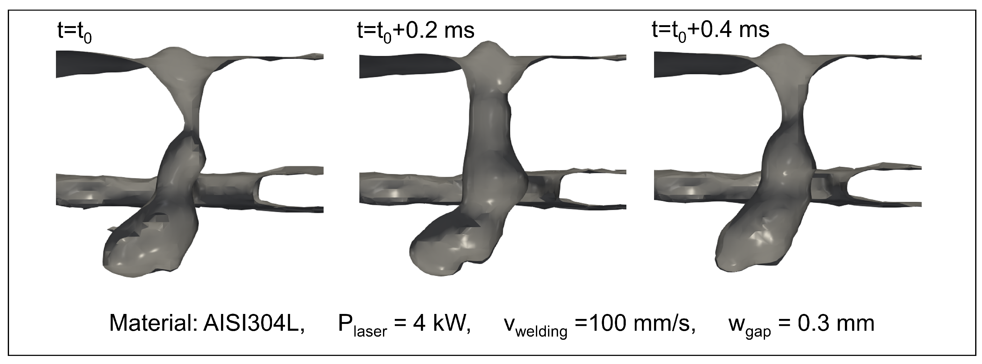
The parameters used for simulation S5, which are used for the discussion of pore formation below, are provided in

Table 4. Conditions of the LBW simulation S5 used for the investigation of the pore formation mechanism.

Parameter	Unit	S5
material	−	AISI304L
sheet thickness	mm	1
welding speed	mm/s	120
laser power	kW	4
laser wavelength	nm	1070
laser M2	−	12.4
laser defocus	mm	7
laser radius on top sheet surface	mm	0.31
gap width	mm	0.45

. A series of longitudinal sections obtained with simulation S5 is provided, with the respective timestamps of the frames, in Figure 12.

The process of pore formation in keyhole laser beam welding starts with a narrow and straight keyhole geometry (Figure 12a). Due to instabilities in the balance of capillary forces and recoil pressure from evaporated metal, caused by the rapidly changing geometry at the locations of inbound laser light, a bulge starts to form, extending into the liquid. As a consequence of fast evaporation and the resulting shear stresses at the liquid-vapor interface, upwards-traveling waves form within the melt. These waves, when their amplitudes reach sufficiently high peaks, can block some laser light from reaching the bottom of the keyhole, and thus condensation occurs in the deepest region of the keyhole, resulting in low pressure pulling in air from the gap between the plates (Figure 12b). Subsequent low-pressure areas form due to further condensation in the region of the lower plate, and thus more ambient gas is sucked in (Figure 12c). The remaining vapor in the cavity at the bottom of the keyhole in Figure 12c fully condensates. After about 0.25 ms, liquid filled the lower part of the gap sufficiently for the absorption at the front wall, and thus evaporation, to increase again. The expanding vapor pushed the now trapped ambient gas further down and towards the back of the keyhole (Figure 12d). Fast moving vapor and constantly changing absorption conditions led to mixing of the evaporated metal and the trapped gas (Figure 12e) and to the formation of a larger bulge. Approximately 0.25 ms later, a larger liquid melt wave in the upper region of the keyhole constricted the opening entirely and thus blocked laser energy from reaching the bulge in the lower plate. This caused fast condensation in the whole region of the gap and the lower plate where metal vapor was present (Figure 12f), and thus much more air szx pulled inwards. Again, increasing evaporation at the front of the keyhole trapped the ambient gas, creating a cavity at the bottom (Figure 12g). When closing was forced due to the surface tension becoming larger than the vapor pressure holding the keyhole open, it constricted, forming a pore (Figure 12h). If said pore is not formed far enough, or shed with enough momentum, behind the location of the optical axis, it is quickly rejoined with the keyhole and the processes described above repeat. When the pore is large enough and detaches far enough behind the current laser position, it remains stable inside the melt pool, being subject to oscillations due to changes in flow conditions and buoyancy forces (Figure 12i). After some time, the whole process starts again with a new potential pore, while the previous pore has settled in its final position (Figure 12j).

In welding processes, the requirement to have full penetration through both plates to be welded helps the ambient gas trapped inside the pores to escape at the bottom of the lower plate. Therefore, pore formation through the previously described processes is only possible when full penetration is not achieved in all parts of the weld bead length. As seen in Figure 12j), pores are only present where full penetration is not achieved. Increasing the power further would change the dynamics inside the keyhole, leading to a mostly open keyhole at the bottom of the lower plate and disrupting the fine balance described above, so as to hinder pore formation entirely.

5. Conclusions and Outlook

The calibrated and subsequently validated model for keyhole laser beam welding presented in this paper showed its ability to accurately predict weld bead geometries of 304L stainless steel in a timely manner without the use of an unreasonable amount of computational resources, thereby making it a great numerical tool for industrial applications in process investigation, optimization and data collection. Subsequent refinement and the investment of more resources led to the feasibility of using the model for basic research about physical mechanisms inside the material, which are difficult to observe experimentally. Furthermore, its generic programming and the lack of process-specific assumptions allow for quick adaptability and the use of a single model to simulate different processes (laser ablation, laser scribing, laser drilling, laser-based additive manufacturing, etc.), some of which have already been simulated successfully.

In future scientific efforts, an interesting study could be carried out by comparing the discovered mechanisms of pore formation to experimental data and also investigating the wave generation and propagation inside the liquid material more in depth. A further comparative study between the herein predicted optimal beam shapes and a real-world application will be a product of the CUSTODIAN project.