1. Introduction
Currently, knee replacement surgery is performed on a large number of people throughout the world. Modern technologies would be required to contribute to this subject within the near future. This means that techniques used for virtual prototyping of mechanical systems must be extended to advanced biomechanical systems to meet the specifications and demands [
1,
2,
3,
4,
5,
6,
7].
The most efficient process for correcting deformities in the leg and removing pains associated with the knee, and enabling sanctionative patients to resume traditional daily activities, is by Total knee replacement (TKR) surgery. Since the primary TKR surgery was performed in 1968, enhancements with different materials and methods have drastically increased its effectiveness [
7,
8,
9,
10,
11].
The proper handling of degenerative abrasion in the knee joint is currently one of the essential orthopaedic problems. The appropriate solution for this issue is to remove and replace it with a prosthesis. Unfortunately, no perfect knee prosthesis is available to replace the original knee because of the knee kinematics’ complexity.
Results for the kinematical design method of the knee prosthesis geometries by Balassa, 2019, compared to the normal human knee [
12], shows that the basic principle of their method was to move the two prosthetic components together according to the objective function of flexion and rotation of the knee prosthesis. The results showed a close match with the curve of the movement of the normal human knee.
The test machine for measuring the prosthesis by Balassa, 2019, was created by the Biomechanical Research Group of Szent Istvan University. With this machine, they made many different sizes of the prosthesis by using the 3D model of knee prosthesis. The developed prosthesis model was produced by the CNC milling technology [
12].
The test machine is multipurpose, making it ideal for evaluating the knee prostheses. Its suitability for different types of loads is also significant.
Unfortunately, in using the method of machine milling with 3D printing, designing and developing the knee prosthesis is time-consuming, and a high cost is incurred. Since it is a try and error method, and there is no predefined procedure, a significant quantity of knee prosthesis model material will be lost with these measurements [
13,
14].
Fekete et al. used the 3D computational model in the MSC.ADAMS software to examine the forces that connect the surfaces of the femur, tibia, and the patella. They applied the equilibrium equations by defining the forces relating to the femur, tibia, and the patella. In the end, they obtained the force functions as inputs for the isometric motions. However, the internal forces connecting the surfaces as a function for flexion were not investigated [
15,
16,
17].
The application of the MSC.ADAMS software for our study made use of the linear or non-linear ordinary differential equations simultaneously with the non-linear differential algebraic equations. To find a solution with these equations, an initial value is determined from which the final trajectory would be determined [
15]. Thus, the appropriateness of using the ADAMS programme to design the knee prosthesis as a faster, more efficient and accurate procedure without having to go through the several testings attempts to arrive at the appropriate design as done in the procedure by [
12].
This study aims to develop the numerical measurement of the knee prosthesis geometry by applying the MSC.ADAMS program. The forces that relate to the femur, tibia, and the patella would be investigated. The 3D CAD printing procedure will be applied to create the initial knee prosthesis, and then the ADAM software used to model and obtain the final product. The results would then be compared with the outcome from the 3D CAD model and CNC milling process, and the prosthesis results from a test rig. The proposed research is thus, to obtain the knee prosthesis by applying a more efficient procedure devoid of material and time wastage and minimize cost.
2. Materials and Methods
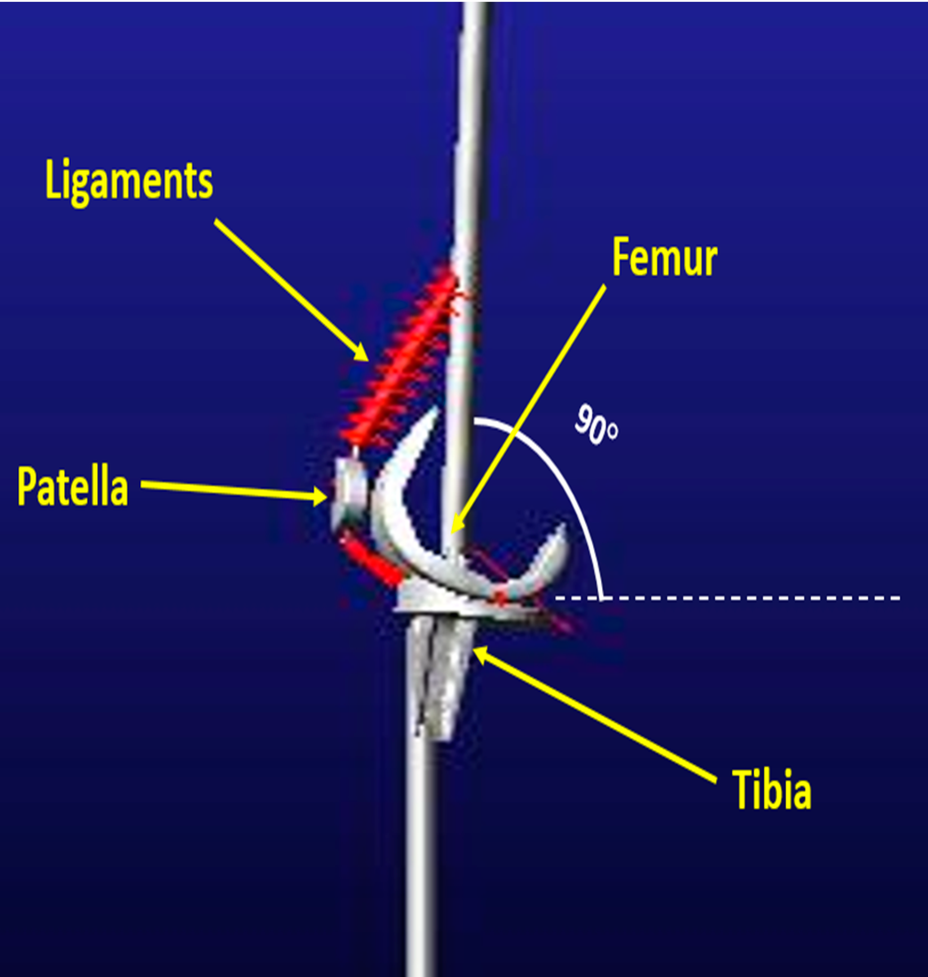
Generally, for the typical normal human knee flexion or extension, the patellofemoral joint’s local kinematics can be classified as partial rolling and sliding. The associated movement is controlled by connecting the tibial surfaces, the femoral, and the ligaments.
The exact relationship of the sliding rolling phenomenon regarding the knee’s typical functional arc has still not been ascertained. However, it has been used by the early works of [
18,
19]. Between the angles of 20–30° of flexion, rolling appears to be more significant, while beyond these angles, the sliding angle becomes more prevailing [
20,
21].
The “Screw home mechanism”, which occurs in the arc between 0° and 20°, is of tremendous interest for an anatomist, although it may have little benefit in the daily living activities and activities such as one-legged stance or normal stance [
22,
23].
In the current work, the maximum arc angle of 110° was considered. This is because there is no increase in the patellofemoral forces above 120° of flexion. Also, in areas like Asia, where it appears in part of their cultures, its relevance is insignificant [
24,
25].
2.1. Knee Joint Geometry
The tibia, patella, and femur were taken to be rigid bodies as the effect of deformation is not considered in this study. The femur and tibia geometry was based on the prosthesis prototypes developed by Balassa 2019, as shown in
Figure 1 and
Figure 2. These designs are still being researched and refined. The designed samples of the prosthesis are shown in
Figure 1 and
Figure 2. As the basis for our model in the ADAMS software, these initial prosthesis prototypes were transferred together with the 3D model into the ADAMS programme as the initial framework for the prosthesis design. The obtained STL file is converted to an IGS file and finally into the PARASOLID format for application in the ADAMS program.
2.2. Ligaments and Muscles
The various ligaments and the muscle are designed as simple linear springs. Considering both the ligaments and the muscles only in arithmetic, the stiffness modulus is set to 130 N/mm and the damping modulus to 0.15 Ns/mm in the case of both springs.
2.3. Mu Static
The coefficient of friction is the standard describing the force of friction between 2 objects and the natural reaction found for the objects in question. This value is used to determine the friction force of an object [
26,
27] and when using other methods as shown in Equation (1), the coefficient of friction.
where
The frictional force
The coefficient of friction
The normal force.
stands for different items. It can be the coefficient of Static friction , and also the coefficient of dynamic friction.
The expression for the frictional force is shown in Equation (2):
2.4. Mu Dynamic
Strong friction opposes the lateral sliding movement between two objects in contact; they are divided into two main groups, static friction occurs between stationary objects, and kinetic friction occurs between objects or surfaces in motion as it is called (dynamic friction) (Air, 1921).
Coulomb friction is applied to dry friction, and the expression for its determination is presented in Equation (3):
where
is the frictional force resulting from the collision of the two surfaces and the application of the forces to each other. It is in line with the surface and applied in the opposite of the force.
is the coefficient of friction; this reveals the relationship and the normal reaction that exists between two bodies.
is the average force obtained on each surface, directed perpendicular to the surface.
The value of the Mu dynamic frictional force chosen for the modelling is 0.3, as shown in
Table 1.
2.5. Description of the Calculations Employed in the ADAMS Model
In this section, the kinematic calculations for the motion as a function of time and automatically solved by the ADAMS programme are presented.
Because the multibody is considered solid, the solid body kinematics is applicable. The ration of the sliding roll is determined only between the femur and the tibia. This is what was noticed, that the patella does not appear in the account or the figures. The following Equations (4)–(6) were used to determine the velocity at a point of the connecting femoral or tibial surfaces (
Figure 3).
where,
By substituting Equation (5) into (4), we obtain:
From Equation (5), we obtain (7) and (8):
Velocities relating to the femur and tibia at the point of contact have been determined in the absolute coordinate system (
Figure 4).
At the unit vector
we multiply Equations (7) and (8):
The tangential scalar components are justified only under the following condition [
28].
This indicates that the typical normal standard components of the femoral and tibia contact velocities should be the same. Otherwise, there would be a collision or separation of the two surfaces.
By combining scalar velocities over time, the length of the continuous arc with respect to the femur and tibia can be calculated as follows:
The sliding scroll ratio can be entered back by specifying the arc lengths on both connected bodies:
where,
These rates show the differences increasing with the longest connected arc.
The sliding rolling ration is the difference between the distance travelled () on the tibia and the additional distance travelled () on the femur bone over the increased distance travelled () on the tibia. N shows the arc length during the connection.
Thus, we can conclude accurate calculations about the sliding and gradient features of motion. The sliding toll ratio that translates to zero means this is pure rolling. Regarding a ratio between 0–1, the movement turns into partial rolling and sliding.
Determining the sliding roll ratio as a function of the bending angle is better than determining it as a function of time. We will explain what we have done with this sliding rolling ratio. The flexion angle (γ) was derived, adding the femur and tibia’s angular velocities around the X-axis, and was set to an initial degree of 20° of squatting.
By defining a function, the time can be altered by the angle of flexion, and rolling can be plotted in correlation with the angle of flexion.
2.6. The Multibody Model
The multibody model was created by applying the following procedures
The general point motion was used to stabilize the distal femur, where all the coordinates are shown (
Figure 5). This enables the distal femur to make a transitional movement along the y-axis.
The cylindrical joint model was used to restrict the knee part to allow rotation around all axes (
Figure 5). This enables the shin bone to conduct a natural rotation.
We only considered the patellar tendon and the rectus femur in the numerical-kinematical model. We create both of them as simple linear springs. According to the literature, the rectal femoral stiffness modulus was determined between 25 and 100 N/mm, according to the literature [
29,
30]. As an average value, we set it to 80 N/mm. With the stabilization factor set at 0.15 Ns/mm, for all the strings to prevent oscillations in the system, the patellar tendon was set to inextensible (
Figure 5).
According to Coulomb’s law, contact restrictions are established concerning static and low dynamic friction coefficient (µs = 0.4 µd = 0.3) between the femur, tibia, and patella, similarly to real joints. The kinetic relationship between systemic forces, frictional forces (Fn, Fs), and flexion angle is analyzed using this constraint.
2.7. Boundary Conditions for the Simulation
After the geometrical model is obtained, the MSC.ADAMS program was used to build the multibody model. The following boundary conditions were applied to our model (prosthesis geometry):
Figure 6 presents the flow chart of the applied steps of the multibody virtual model created in the ADAMS software
After the validation and acceptance of the results, the application stage will be to print the femur and the tibia by using 3D printing as in
Figure 7.
3. Results and Discussion
This section presents the results and the accompanying discussions for the study. The movement of the knee in the sagittal plane (lateral movement), flexion position, and the last stage of extension, and in the medial rotation or transverse motion are presented in the flexion and rotation diagrams. Thus, showing the measured ranges of the flexion and extension and rotation of the knee prosthesis during the simulation process. These figures are, in essence, used to determine the point of sliding and rolling.
3.1. The Virtual Multibody Model
The ADAMS programme could compute the forces directly. At first, we saved it as PARASOLID, and we imported it into the MSC.ADAMS. The flexion angle was derived by combining the femur and tibia’s angular velocities about the x-axis. This was done considering that the model was at 20° for the sliding and rolling at the start of the movement. The angles were divided into three to tackle the three-dimensional movement. The results are summarized in
Figure 8.
To be able to describe all the coordinates, we have restricted the distal femur by the general point motion, as shown in
Figure 8. The knee model was restricted by a cylindrical joint, which allows the flexion process between a femur and tibia. Simple linear springs are designed as the boundary between the rectus femur and the patellar tendon [
29,
30].
According to Coulomb’s law, the limitations of contact between the femur and the patella tibia are established for low static and dynamic friction coefficients (μs = 0.4 μd = 0.3), similar to human joints [
31]. A force vector was created on the femur distal, as shown in
Figure 9, and the value set at 800 N, while defining it by a step function (A, x0, h0, x1, h1).
3.2. Simulation of the Multibody Model in Different Positions
3.2.1. Simulation of the Multibody Model at the Position of 25°
The simulated model is shown in
Figure 9. The graph of rotation against flexion is illustrated in
Figure 10. It was noticed that the angle of rotation varies linearly with respect to the flexion. It was observed that the sudden increase in the rotational angle was offset by an increase in the angle of curvature. A sharp rise in the flexion angle till 25° was seen beyond the rotational angle of 20°. The maximum elevation of flexion against the angle of rotation was found to be 25°.
3.2.2. Simulation of the Multibody Model at the Position of 50°
The simulated model and the graphical representation of the rotational angle with flexion are depicted in
Figure 11 and
Figure 12, respectively. It was observed that there was an increase in the degree of rotation (virtual axis) from 0 to 9.5°, whereas the flexion (horizontal axis) varies until 50°. The flexion angle’s relative variation was five times bigger than the rotational angle, which indicates that the onset of sliding between the tibia and the femur in the knee occurs in the range of 20–30° of flexion angle, which conforms with the movement range of the normal human knee.
3.2.3. Simulation of the Multibody Model at the Position of 100 Degrees
The pictorial representations of the model at the angles of 0° and 100° of flexion are shown in
Figure 13 and
Figure 14. The relationship between the angles of rotation and flexion is illustrated in
Figure 15. It is observed that the sudden increase in the rotational angle was offset by an increase in the angle of curvature. A sharp rise in the flexion angle till 35° was seen beyond the rotational angle of 20°, which indicates the onset of sliding between the tibia and the femur in the knee. Similarly, the flexion angle in the range of 20–30° originates the joint prone to rolling. In contrast, the rotational angle’s stability for the flexion angle lies in the range of 30–110°. The increasing flexion angle indicates that the tendency of sliding is predominant.
3.2.4. Experimental Measurement Result for Test Machine of Szent Istvan University
The result shown in
Figure 16 is essential as it is the basis for our numerical experimentation. The research team of Szent Istvan University developed several prosthesis design methods initiated by [
12] using the test machine they developed, as shown in
Figure 17. It was mentioned by Balassa, 2019, that the presented results in his study was the best with respect to the closeness to the real knee movement.
3.2.5. Comparing the Results of the Current Study of the Numerical Measurement Method and the Experimental Measurement Result for the Test Machine of Szent Istvan University
In order to validate the results from the numerical studies, we compared our virtual numerical model with the prostheses joints that have been tested using the test machine in Szent Istvan University. The average values (
Figure 18) are plotted together against the virtual numerical model, as shown in
Figure 19. The close similarity between the two curves indicates that this virtual model can replace the Szent Istvan University test machine’s measurement.
It was also found that there was a rise in the angle of rotation as the flexion angle varied from 0 to 30°. A good agreement of value obtained from our model with other prosthetic joints is established in the flexion range of 30–110°.
We noticed the same results for the proposed model and other prostheses. In this case, we were able to create a new model that enables us to make multiple measurements. We could change the materials made of artificial joints, make them more accessible, and obtain faster results without many calculations. A comparison of our model with the test machine is presented in
Table 2.
4. Conclusions
It can be said that the application of the multibody model saves time as there is no involvement of the tibia and femur, as needed for the knee prosthesis. More importantly, as the application of the test machine is omitted in our process, our model’s approximations to a human knee are carried out directly. Without cost, we can make several measurements for a person’s knee size to be repaired.
The MSC.ADAMS programme was applied to determine the human knee joint’s movement in terms of rotation and flexion. The relationship between these two processes was also described. The changes between the condyles of the developed multibody of the prosthesis are also investigated concerning the flexion angle ranging from 20–120°. The boundary conditions were determined, and simulations performed using the ADAM’s programme. Three-dimensional geometry was applied in the new virtual model, taking into account the influence of the condyles and collateral. The multibody modelling was used to measure the degree of flexion and rotation of the knee concerning its position, like extension, flexion or rotation, and insert a spring between the tibia and femur while observing its effects on the performance of the knee.
A slip ration, which is higher than 0.45, was achieved as was the limit in literature. Applying our model, an average value of 0.7 was reached, with the maximum reaching up to 0.79 and obtaining an angle between 110–120° for the flexion angle. The generated virtual model was used to measure the knee prosthesis size before its creation.
Finally, this virtual model could be used to measure the knee prosthesis size before creating it because it saves time, money, and effort instead of using 3D printing technology, and CNC milling consumes our time, money, and effort.
In future work, we will try to create a virtual model for the ankle to obtain a new virtual model for the complete human leg with the knee and ankle and all required movements. Analysis of the anatomical angles, such as the different rotation as human full legs, abduction, and adduction, will be conducted.
Author Contributions
Conceptualization, K.Z.; methodology, K.Z.; software, K.Z.; validation, K.Z. and O.I.; formal analysis, K.Z.; investigation, K.Z.; resources, K.Z.; data curation, K.Z.; writing—original draft preparation, K.Z.; writing—review and editing, K.Z. and O.I.; supervision, O.I.; funding acquisition, O.I. All authors have read and agreed to the published version of the manuscript.”
Funding
This research received no external funding.
Institutional Review Board Statement
Not applicable.
Informed Consent Statement
Not applicable.
Data Availability Statement
Not applicable.
Acknowledgments
This work was supported by Stipendium Hungricum, and the Szent István University, Gödöllö, Hungary. Faculty of Mechanical Engineering and Mechanical Engineering PhD School.
Conflicts of Interest
The authors declare no conflict of interest.
References
- Zanasi, S. Innovations in total knee replacement: New trends in operative treatment and changes in peri-operative management. Eur. Orthop. Traumatol. 2011, 2, 21–31. [Google Scholar] [CrossRef] [PubMed][Green Version]
- Price, A.J.; Alvand, A.; Troelsen, A.; Katz, J.N.; Hooper, G.; Gray, A.; Carr, A.; Beard, D. Hip and knee replacement 2 Knee replacement. Lancet 2018, 392, 1672–1682. [Google Scholar] [CrossRef]
- Katona, G.; Csizmadia, M.B.; Andrónyi, K. Determination of reference function to knee prosthesis rating. Biomech. Hung. 2015. [Google Scholar] [CrossRef]
- Ardestani, M.M.; Moazen, M.; Jin, Z. The Knee Contribution of geometric design parameters to knee implant performance: Con fl icting impact of conformity on kinematics and contact mechanics. Knee 2015, 22, 217–224. [Google Scholar] [CrossRef]
- Feng, J.E.; Novikov, D.; Anoushiravani, A.A.; Schwarzkopf, R. Total knee arthroplasty: Improving outcomes with a multidisciplinary approach. J. Multidiscip. Healthc. 2018, 11, 63–73. [Google Scholar] [CrossRef] [PubMed]
- Coppolecchia, A.; Cool, C.; Jacofsky, D.; Gregory, D.; Sodhi, N.; Mont, M. Healthcare utilization and payer cost analysis of robotic-arm assisted total knee arthroplasty at 30-, 60-, and 90-days. J. Knee Surg. 2019, 3, 67–72. [Google Scholar] [CrossRef]
- Sasseville, D.; Alfalah, K.; Savin, E. Patch test results and outcome in patients with complications from total knee arthroplasty: A consecutive case series. J. Knee Surg. 2019, 1. [Google Scholar] [CrossRef]
- Vince, K.G. The problem total knee replacement systematic, comprehensive and efficient evaluation. J. Bone Jt. Surg. 2014, 96, 105–111. [Google Scholar] [CrossRef]
- Bert, J.M. Unicompartmental knee replacement. Orthop. Clin. N. Am. 2005, 36, 513–532. [Google Scholar] [CrossRef] [PubMed]
- Bull, A.M.J.; Kessler, O.; Alam, M.; Amis, A.A. Changes in knee kinematics reflect the articular geometry after arthroplasty. Clin. Orthop. Relat. Res. 2008. [Google Scholar] [CrossRef]
- Schwarze, M.; Schonhoff, M.; Beckmann, N.A.; Eckert, J.A.; Bitsch, R.G.; Jäger, S. Femoral cementation in knee arthroplasty—A comparison of three cementing techniques in a sawbone model using the ATTUNE knee. J. Knee Surg. 2019, 1. [Google Scholar] [CrossRef]
- Balassa, G.P. Development and examination of a knee prosthesis geometry. Műszaki Tud. Közl. 2019, 11, 27–30. [Google Scholar] [CrossRef][Green Version]
- Chui, C.S.; Leung, K.S.; Qin, J.; Shi, D.; Augat, P.; Wong, R.M.Y.; Chow, S.K.H.; Huang, X.Y.; Chen, C.Y.; Lai, Y.X.; et al. Population-based and personalized design of total knee replacement prosthesis for additive manufacturing based on chinese anthropometric data. Engineering 2020. [Google Scholar] [CrossRef]
- Zhou, F.; Xue, F.; Zhang, S. The application of 3D printing patient specific instrumentation model in total knee arthroplasty. Saudi J. Biol. Sci. 2020, 27, 1217–1221. [Google Scholar] [CrossRef] [PubMed]
- Fekete, G.; Wahab, M.A.; Baets, P.D. Analytical and computational estimation of patellofemoral forces in the knee under squatting and isometric motion. Sustain. Constr. Des. 2011, 2, 246–257. [Google Scholar]
- Quinlan, N.D.; Wu, Y.; Chiaramonti, A.M.; Guess, S.; Barfield, W.R.; Yao, H.; Pellegrini, V.D. Functional flexion instability after rotating-platform total knee arthroplasty. J. Bone Jt. Surg. 2020, 102, 1694–1702. [Google Scholar] [CrossRef]
- Zeng, Y.M.; Yan, M.N.; Li, H.W.; Zhang, J.; Wang, Y. Does mobile-bearing have better flexion and axial rotation than fixed-bearing in total knee arthroplasty? A randomised controlled study based on gait. J. Orthop. Transl. 2020, 20, 86–93. [Google Scholar] [CrossRef] [PubMed]
- Zuppinger, H. Die aktive Flexion im unbelasteten Kniegelenk. Die aktive Flexion im unbelasteten Kniegelenk 1904. [Google Scholar] [CrossRef]
- Braune, W.; Fischer, O. Die bewegungen des Kneigelenkes nach einer neuen Methode am lebendon menschen Gemessen. Des XVII, Bandes der Abhand lungen der Mathematisch. Phys. Cl. Konigl. 1891, 17, 75–150. [Google Scholar]
- Abid, M.; Mezghani, N.; Mitiche, A. Knee joint biomechanical gait data classification for knee pathology assessment: A literature review. Appl. Bionics Biomech. 2019, 2019. [Google Scholar] [CrossRef]
- Zhang, L.; Liu, G.; Han, B.; Wang, Z.; Yan, Y.; Ma, J.; Wei, P. Knee joint biomechanics in physiological conditions and how pathologies can affect it: A systematic review. Appl. Bionics Biomech. 2020, 2020. [Google Scholar] [CrossRef]
- Cerulli, G.; Amanti, A.; Placella, G. Case report surgical treatment of a rare isolated bilateral agenesis of anterior and posterior cruciate ligaments. Case Rep. Orthop. 2014, 2014, 809701. [Google Scholar]
- Smith, B.J.W. Observations on the postural mechanism of the human knee joint. J. Anat. 1954, 90, 236–261. [Google Scholar]
- Csizmadia, B.M.; de Baets, P.P. Kinetics and Kinematics of the Human Knee Joint under Standard and Non-Standard Squat Movement Kinetica en Kinematica van het Humane Kniegewricht Gusztáv Fekete; Ghent University: Ghent, Belgium, 2013; ISBN 9789085785934. [Google Scholar]
- Koh, Y.G.; Park, K.M.; Kang, K.T. Finite element study on the preservation of normal knee kinematics with respect to the prosthetic design in patient-specific medial unicompartmental knee arthroplasty. Biomed. Res. Int. 2020, 2020. [Google Scholar] [CrossRef]
- Zhang, H. Surface Characterization techniques for polyurethane biomaterials. In Advances in Polyurethane Biomaterials; Elsevier Ltd.: Amsterdam, The Netherlands, 2016; pp. 23–73. ISBN 9780081006221. [Google Scholar]
- Liquide, A.; Systems, M. The effect of variable relative insertion orientation of human knee bone ligament bone complexes on the tensile stiffness. J. Biomech. 2016, 30328, 1–17. [Google Scholar]
- Nagy, D.; Szendrő, P.; Nagy, J.; Bense, L. Research & Development. In Proceedings of the Synergy 2015 International Conference, 2015; Volume 13, pp. 21–28. Available online: https://www.gek.szie.hu/english/sites/default/files/rd_mechanical_engineering_letters_vol13_Synergy_selected.pdf (accessed on 8 March 2021).
- Thelen, D.G.; Chumanov, E.S.; Best, T.M.; Swanson, S.C.; Heiderscheit, B.C. Simulation of biceps femoris musculotendon mechanics during the swing phase of sprinting. Med. Sci. Sports Exerc. 2005, 37, 1931–1938. [Google Scholar] [CrossRef] [PubMed]
- Frigo, C.; Pavan, E.E.; Brunner, R. A dynamic model of quadriceps and hamstrings function. Gait Posture 2010. [Google Scholar] [CrossRef] [PubMed]
- Merkher, Y.; Sivan, S.S.; Etsion, I. A rational human joint friction test using a human cartilage-on-cartilage arrangement a rational friction test using a human cartilage on cartilage arrangement. Tribol. Lett. 2006. [Google Scholar] [CrossRef]
| Publisher’s Note: MDPI stays neutral with regard to jurisdictional claims in published maps and institutional affiliations. |
© 2021 by the authors. Licensee MDPI, Basel, Switzerland. This article is an open access article distributed under the terms and conditions of the Creative Commons Attribution (CC BY) license (http://creativecommons.org/licenses/by/4.0/).


