A Comparative Study of Energy Consumption and Recovery of Autonomous Fuel-Cell Hydrogen–Electric Vehicles Using Different Powertrains Based on Regenerative Braking and Electronic Stability Control System

Abstract

Today, with the increasing transition to electric vehicles (EVs), the design of highly energy-efficient vehicle architectures has taken precedence for many car manufacturers. To this end, the energy consumption and recovery rates of different powertrain vehicle architectures need to be investigated comprehensively. In this study, six different powertrain architectures—four independent in-wheel motors with regenerative electronic stability control (RESC) and without an RESC, one-stage gear (1G) transmission, two-stage gear (2G) transmission, continuously variable transmission (CVT) and downsized electric motor with CVT—were mathematically modeled and analyzed under real road conditions using nonlinear models of an autonomous hydrogen fuel-cell electric vehicle (HFCEV). The aims of this paper were twofold: first, to compare the energy consumption performance of powertrain architectures by analyzing the effects of the regenerative electronic stability control (RESC) system, and secondly, to investigate the usability of a downsized electrical motor for an HFCEV. For this purpose, all the numerical simulations were conducted for the well-known FTP75 and NEDC urban drive cycles. The obtained results demonstrate that the minimum energy consumption can be achieved by a 2G-based powertrain using the same motor; however, when an RESC system is used, the energy recovery/consumption rate can be increased. Moreover, the results of the article show that it is possible to use a downsized electric motor due to the CVT, and this powertrain significantly reduces the energy consumption of the HFCEV as compared to all the other systems. The results of this paper present highly significant implications for automotive manufacturers for designing and developing a cleaner electrical vehicle energy consumption and recovery system.

1. Introduction

In the automotive industry, new vehicular technologies such as battery electric vehicles (BEVs), hybrid electric vehicles (HEVs), and hydrogen fuel-cell electric vehicles (HFCEVs) offer critically important environmentally friendly solutions for achieving zero net carbon emissions [1,2,3,4,5,6]. In this regard, HFCEVs have gained special attention owing to their greater charge time–range ratios as compared to BEVs [7]. However, HFCEVs are costly, primarily due to the high production cost of hydrogen fuel. Additionally, the HFCEV demonstrates lower efficiency than the BEV [8,9]. Nevertheless, many manufacturers foresee a reduction in hydrogen fuel costs as cheaper production methods are explored using investments from the solar and wind renewable energy sectors [10,11,12]. The general structure of an HFCEV consists of six major components: a hydrogen storage tank, an air intake system, a fuel-cell system, power electronics, a battery or capacitor, and an electric motor. All these major components directly affect the overall efficiency of the vehicle. The common energy sources available for use in electric vehicles are lithium-ion batteries, supercapacitors, and hydrogen fuel cells. For creating an efficient energy system, each energy source needs to be examined separately, along with studies focusing on hybrid systems that utilize more than one energy source. Hybrid systems offer the advantage of avoiding disadvantages associated with each energy system [13,14,15,16]. In general, hydrogen-powered electric vehicles require an auxiliary energy storage system in the vehicle during energy recovery. Therefore, electric vehicles with hydrogen fuel cells require additional batteries or supercapacitors. A supercapacitor acts as a buffer against sudden charging currents, maintaining the overall efficiency, which makes it a more viable choice for use in vehicles to achieve energy recovery as compared to batteries [17,18].

In an electrical vehicle, the electrical motor is generally connected to the wheels through a single-stage transmission path. This simple and relatively economical design is called a two-wheel-drive layout. However, different powertrain architectures are also available, such as an in-wheel motor and four-wheel-drive layouts with multistage gearbox systems. The mechanical layout design is a critically important factor in assuring optimal energy consumption and recovery rates for the electric motor. It also directly determines other parameters such as the size of the electrical motor, power of the fuel cell, and tank capacity, etc. A two-wheel-drive design also allows the construction of a more efficient, lighter, cheaper, and lower-volume electric motor due to the reduction in the rotor size and stator geometries of the electric motor. For analyzing mechanical layouts based on energy consumption and recovery performance, numerous studies have been carried out [19,20,21,22]. Bottiglione et al. [23] created an energy consumption model of an electric vehicle for comparing one-stage (1G) and two-stage (2G) gear drives, half and full toroidal continuously variable transmissions (CVTs), and two different types of infinitely variable transmissions (IVTs). In the research, the energy efficiencies of the electric motor and transmission of six different transmission types of EVs were calculated. In another piece of research, Sluis et al. [24] described the advantages of using a single-loop set belt CVT as compared to using 1G, 2G automatic, and 2G double-clutch transmission based on a comparison of their values of energy consumption, cost, and performance in a downsized electric motor. Furthermore, other studies have focused on innovating shifting strategies in electric vehicles. In particular, efforts have been made to improve energy consumption and recovery to ensure a smooth drive during shifting. Shifting innovations are also used in some clutches used in transfer elements. Particularly, a double clutch enhances the power connection between a motor and powertrain during shifting [25,26,27].

Among the different transmission systems, the continuously variable transmission (CVT) system can increase the efficiency of a powertrain system significantly, as it can continuously change the speed ratio and allows the electric motor to operate around the most efficient regions [28,29,30,31]. Therefore, a CVT system improves the overall performance and motor efficiency of an electric vehicle, whilst also helping to downsize the electric motor and other energy sources [32,33,34,35,36,37,38]. Another major layout for electric vehicles is an independent in-wheel motor with/without a planetary gear. This system offers some key advantages, one of which is greater vehicle control, owing to its all-wheel design, which can be controlled with high precision and speed. Another advantage is the increase in the internal volume of a vehicle due to the removal of the transmission system, which also prevents the power loss of transmission systems [39,40]. Conversely, this type of electric motor increases the mass of the wheel group, thus increasing the unsprung mass, which in turn affects the vehicle drive. The increased mass of the wheel group reduces the fatigue strength of the elements in the suspension system [41]. Nevertheless, the aforementioned advantages of an in-wheel motor, such as regenerative electronic stability control (RESC), have opened up avenues for further exploration. To this end, research by Najjari et al. [42] proposed a strategy for managing the energy and directional stability of four in-wheel-driven electric vehicles. Another piece of research by Xu et al. [43] modeled four in-wheel hub motors by examining factors such as the regenerative braking performance and its effect on energy recovery for the front and rear wheels. In the study, although the in-wheel motor was used as a generator, its performance in influencing the braking conditions and energy consumption rate need to be further examined based on its comparison with the other types of powertrain architecture.

To date, no research has focused on drawing a comparison between the energy consumption performance of an HFCEV equipped with in-wheel-driven motors and that of an electrical motor utilizing CVT and other powertrain layouts based on RESC technology. In addition, a comprehensive comparison has not been performed using a downsized electrical motor. Thus, this study investigated the energy consumption rate and recovery performance of an autonomous HFCEV equipped with six different powertrain architectures: four independent in-wheel motors using RESC and without RESC, one-stage gear (1G) transmission, two-stage gear (2G) transmission, CVT, and a downsized electric motor utilizing CVT. In the mathematical model, the HFCEV was modeled, and simulations were performed for FTP75 and NEDC urban drive cycles. Additionally, the total energy consumption of the HFCEV with different powertrains was compared. The results demonstrate that the minimum energy consumption can be obtained with 2G transmission for the same motor. In this regard, a regenerative electronic stability control system can increase the energy recovery/ consumption rate of the HFCEV by at least 3%. Furthermore, the results illustrate that it is possible to reduce the size of the electric motor by using CVT, as the required maximum peak torque can be reduced. The simulations were repeated using a downsized electric motor, and the value for the best energy consumption was obtained owing to the light components of the system.

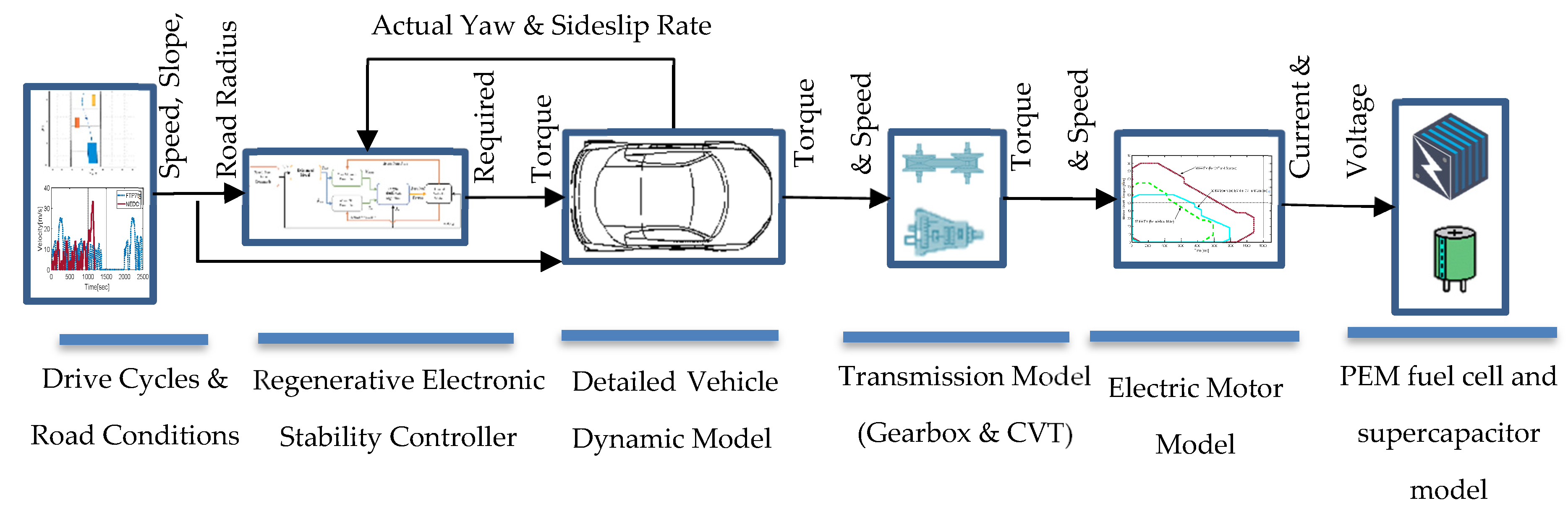
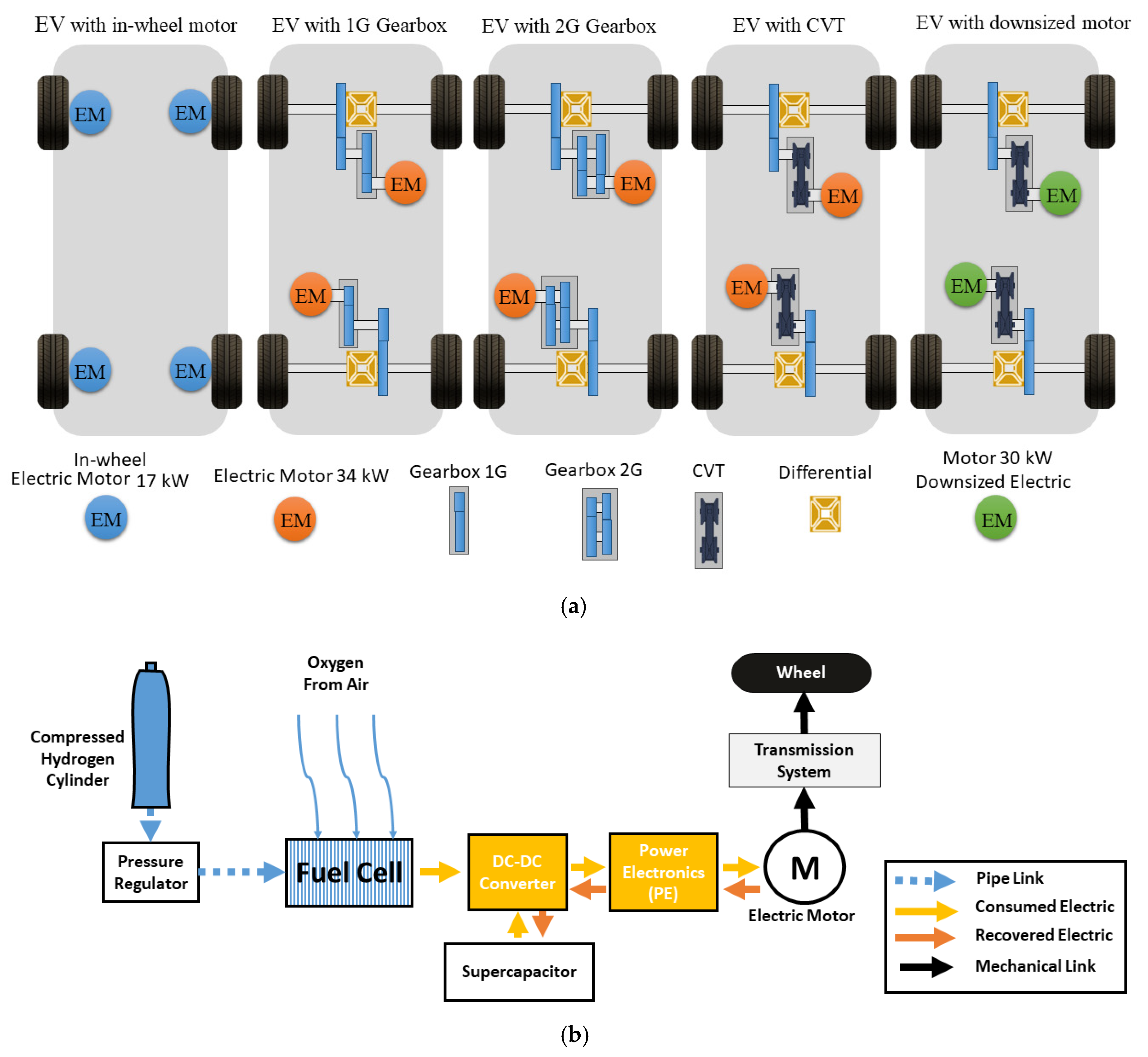
2. Developed Simulation Model for Different Powertrain Layouts

In this section, the details of the developed simulation model are presented. Mathematical formulations were developed based on the block diagram that is shown in Figure 1. The model included the drive cycles, an RESC controller, dynamic equations for the vehicle, transmission models, electrical motor maps, and formulations of the subsystems. It should be noted that the RESC controller was only available in the in-wheel motor driven powertrain architecture, and that the developed model was found to be suitable for all the different types of powertrain architectures used for HFCEVs.

Based on Figure 1, firstly, the necessary powers and torques for the FTP75 and NEDC drive cycles were calculated, and then, these values were used in the electric motor model. For all types of electric motors, the efficiency was determined from real-life working conditions, and the current and voltage were calculated based on the necessary torque with respect to the angular velocity. After defining the current and voltage of the electrical motor, the energy consumption and recovery were determined based on the proton exchange membrane PEM fuel cell and supercapacitor model. At the end of the calculation, the values for the other parameters, such as the energy consumption, energy recovery, and operating points on the efficiency maps, were obtained for all the types of powertrain layouts for HFCEVs.

In Figure 2, different powertrain layouts and an energy supply diagram for the HFCEV are presented for drawing comparisons between their energy consumption and recovery rates. As shown in Figure 2a, there are four main layouts. The first type of vehicle is equipped with four permanent magnets synchronous with the in-wheel electric motor. In the second, third, and fourth models, there are two main central electric motors, and they are coupled with different types of transmission systems: one-stage (1G) and two-stage gear ratios (2G), continuously variable transmission (CVT), and downsized electric motors with CVT. The speed ratios of the one-stage and two-stage automatic gearboxes were defined by considering the optimum operating conditions of the electric motor with regard to the efficiency map of an electric motor (in the Appendix A). Additionally, the efficiency values of the transmission, system were also considered. Furthermore, an energy supply diagram for the HFCEV is illustrated in Figure 2b. The main energy source of the vehicle is defined as a PEM fuel cell, and its output directly connects to 255 V DC–DC boost converters. A supercapacitor is an auxiliary energy source and serves as the energy recovery unit of the vehicle.

The case study vehicle was an urban autonomous passenger car. As shown in Figure 3, the selected vehicle model was shown considering its steering angle, suspension, calculations of resistance forces $F_l$ (aerodynamic drag, tire rolling resistance, and slope), and efficiencies of the mechanical and electrical components.

The sum of the load forces that were used are given as follows:

$$F_l=\rho c_d{A}_f\frac{v_{}{}^2}{2}+m_{t}g\sin \left(\beta \right)+m_{t}g\left(f_0+f_1{v}^2\right)$$

(1)

Here,$v,$ $m_t,\beta$, $A_f$, $c_d$, and $\rho$ indicate the velocity of the vehicle, the total mass of the vehicle, the slope angle of the road, the frontal area, the drag coefficient, and the air density, respectively. Note that, total mass of the vehicle is sum of the vehicle mass without transmission layout $m_v$ given in

Table 1. Specifications of the selected autonomous electric vehicle.

Drag coefficient	${\mathrm{c}}_{\mathrm{d}}$	0.32	Half length of vehicle	$\mathrm{l}$	1.413 [m]
Frontal area	${\mathrm{A}}_{\mathrm{f}}$	1.4 [${\mathrm{m}}^2$]	Half width of vehicle	$\mathrm{w}$	0.652 [m]
Vehicle mass inertia at x axis	$I_{xx}$	750 [kg/${\mathrm{m}}^2$]	Wheel radius	${\mathrm{R}}_{\mathrm{w}}$	0.325 [m]
Rolling stiffness coefficient	${\mathrm{K}}_{\mathrm{roll}}$	85,450 [Nm/rad]	Air density	$\rho$	1.225 [kg/${\mathrm{m}}^2$]
Height of the rolling axis	${\mathrm{h}}_{\mathrm{roll}}$	0.27 [m]	Rolling damping coefficient	${\mathrm{C}}_{\mathrm{roll}}$	4542 [Nms/rad]
Vehicle mass (without powertrain and motor)	$m_v$	2300 [kg]	Vehicle mass inertia at z axis	$I_{zz}$	2707 [kg/${\mathrm{m}}^2$]

. $f_0$ and $f_1$ are the coefficients of the rolling resistance constants with values that equal 0.015 and 0.0067, respectively.

In this study, an autonomous vehicle was chosen to subtract the consideration of driver mistakes and steering response delays in the vehicle. Autonomous vehicles can be used to calculate the curvature of the road in different ways. The referenced vehicle detects the lanes using the image processing sliding window method. This method calculates the radius of the road, $R_r$, given in Equation (2), with respect to the referenced double-lane-change maneuver. The purpose of this maneuver is to achieve a lane change by varying the steering angle in one direction (left) and then the opposite direction, simultaneously, as the vehicle encounters an obstacle.

$$R_r=\frac{{\left[1+{\left(\frac{dy}{dx}\right)}^2\right]}^{3/2}}{\left|\frac{d^{2}y}{d{x}^2}\right|}$$

(2)

Here, x and y are coordinates of the roads when looking from top view. The steering angles of the left and right front wheels, ${\delta }_A$ and ${\delta }_B$, respectively, are represented based on the well-known Ackermann principle for left turning as follows:

$${\delta }_A=\arctan \left(\frac{2l}{\sqrt{R_r{}^2-l^2}-w}\right)$$

(3)

$${\delta }_B=\arctan \left(\frac{2l}{\sqrt{R_r{}^2-l^2}+w}\right)$$

(4)

where $l$ and $w$ indicate the half length and half width of the vehicle, respectively.

The longitudinal ${\lambda }_A$ and lateral slips ${\alpha }_A$ were determined for front left tire $A$ and for the others were calculated using similar equations. During driving situations, the longitudinal and lateral slip angles for the left front tire were calculated as follows:

$${\lambda }_A=\left\{\begin{array}{cc}\frac{V_x-R_w{\omega }_A}{V_x},\hfill & brakesituation\hfill \\ \frac{-V_x+R_w{\omega }_A}{V_x},\hfill & drivesituation\hfill \end{array}\right.$$

(5)

$${\alpha }_A={\delta }_A-\arctan \left(\frac{V_y+\gamma l}{V_x-\gamma w}\right)$$

(6)

In the above equations, $V_x$ and $V_y$ represent the longitudinal and lateral velocities, $R_w$ denotes the radius of the wheel, ${\omega }_A$ indicates the angular speed of the front left wheel, and $\gamma$ represents the yaw rate of the vehicle. In addition, for the calculation of the lateral and longitudinal forces, denoted as $F_y$ and $F_x$ respectively, the Pacjeka model was selected. The Magic Formula of Pacjeka is presented in Equations (7) and (8), respectively:

$$F_{yA}\left({\lambda }_A,{\alpha }_A,{\mu }_A,F_{zA}\right)=\frac{{\sigma }_{yA}}{{\sigma }_{tA}}{F}_{yA0}\left({\alpha }_A,{\mu }_A,F_{zA}\right)$$

(7)

$$F_{xA}\left({\lambda }_A,{\alpha }_A,{\mu }_A,F_{zA}\right)=\frac{{\sigma }_{xA}}{{\sigma }_{tA}}{F}_{xA0}\left({\alpha }_A,{\mu }_A,F_{zA}\right)$$

(8)

All the parameters of these two equations (${\lambda }_A,{\alpha }_A,{\mu }_A,F_{zA}$) are explained in the Appendix A. The equations of the motion of the vehicle are listed as follows for the longitudinal, lateral, yaw, and roll motions, respectively:

$${\dot{V}}_x=V_y\gamma +\frac{\left(F_{xA}cos{\delta }_A+F_{xB}cos{\delta }_B+F_{xC}+F_{xD}\right)}{m_t}-\frac{F_l+F_{yA}sin{\delta }_A+F_{yB}sin{\delta }_B}{m_t}-h_{roll}\gamma \dot{\phi }$$

(9)

$${\dot{V}}_y=-V_x\gamma +\frac{\left(F_{yA}cos{\delta }_A+F_{yB}cos{\delta }_B+F_{yC}+F_{yD}\right)+F_{xA}sin{\delta }_A+F_{xB}sin{\delta }_B}{m_t}-h_{roll}\ddot{\phi }\cos \left(\phi \right)$$

(10)

$$\begin{array}{c}\dot{\gamma }=\frac{1}{I_{zz}}[l\left(F_{xA}sin{\delta }_A+F_{yA}cos{\delta }_A+F_{xB}sin{\delta }_B+F_{yB}cos{\delta }_B-F_{yD}-F_{yC}\right)+\\ w\left(-F_{xA}cos{\delta }_A+F_{yA}sin{\delta }_A+F_{xB}cos{\delta }_B-F_{yB}sin{\delta }_B+F_{xD}-F_{xC}\right)]\end{array}$$

(11)

$$\ddot{\phi }=\frac{1}{I_{xx}}\left[m_s{h}_{roll}\left({\dot{V}}_x+gsin\phi \right)-K_{roll}\phi -C_{roll}\dot{\phi }\right]$$

(12)

Here, $F_{xA}$, $F_{xB}$, $F_{xC}$, and $F_{xD}$ denote the longitudinal force of each tire; $F_{yA}$, $F_{yB}$, $F_{yC}$, and $F_{yD}$ are the lateral force of each tire, while $I_{zz}$ and $I_{xx}$ represent the mass inertias for the z- and x-axis, respectively. The term $\phi$ represents the rolling angle, and $h_{roll}$ is the height of the rolling axis. $m_s$ is sprung mass and it is found subtract of unsprung mass $m_u$ (41 kg for in wheel-motor, 23 kg for others) from total mass $m_t$.

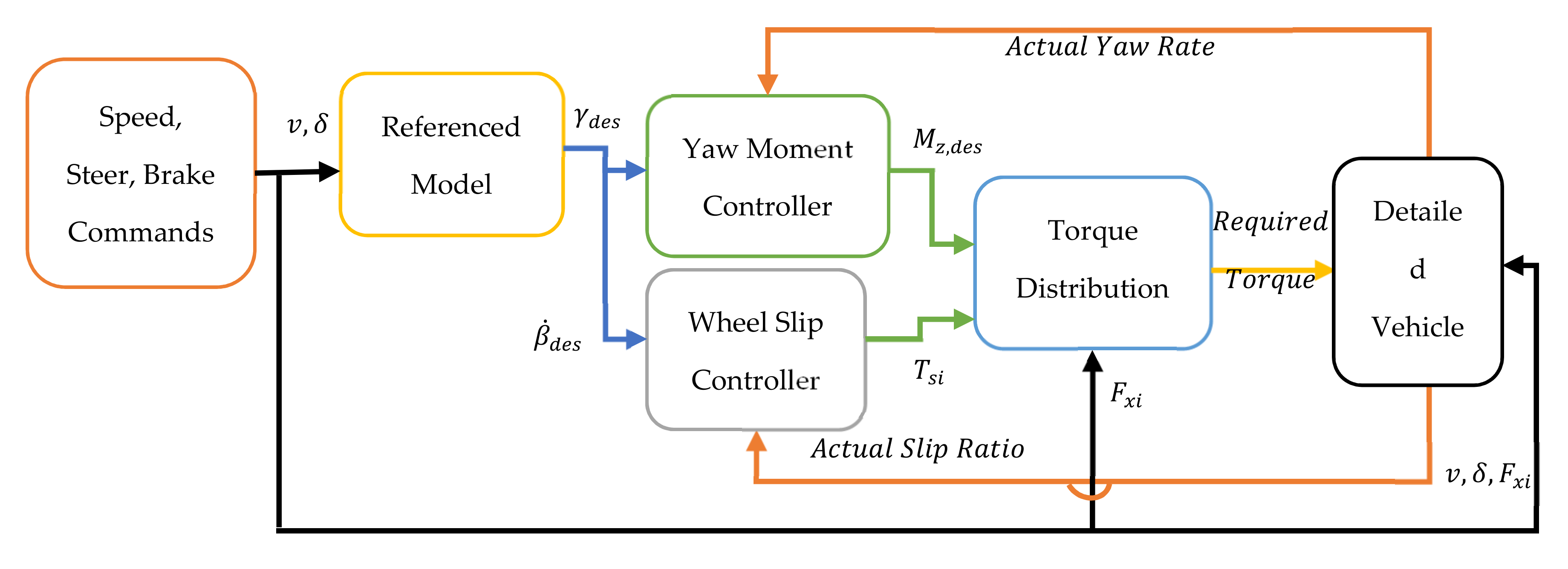
3. Regenerative Electronic Strategy and Stability Control Strategy

The main objective of the yaw rate controller design was to compare the vehicle yaw rate and other stability-related states with the desired states obtained using drive commands of the autonomous vehicles. The desired state parameters –yaw rate and side slip angle- were calculated using a two-DoF vehicle single-track model. The two DoF equations of motion are expressed below.

$${\dot{v}}_{y_d}=\frac{1}{m_t}[\left(C_f+C_r\right)\frac{v_{y_d}}{v_{x_d}}+\left(l{C}_f-l{C}_r-m_t{v}_{x_d}^2\right)\frac{{\gamma }_d}{v_{x_d}}-C_f\delta ]$$

(13)

$${\dot{\gamma }}_d=\frac{1}{I_{zz}}[\left(2l{C}_f-2l{C}_r\right)\frac{v_{y_d}}{v_{x_d}}+\left({\left(2l\right)}^2{C}_f+{\left(2l\right)}^2{C}_r\right)\frac{{\gamma }_d}{v_{x_d}}-2l{C}_f\delta ]$$

(14)

Here, ${\gamma }_d$ desired yaw rate, ${\dot{v}}_{y_d}$ desired lateral acceleration, ${\dot{v}}_{x_d}$ desired longitudinal acceleration, $C_f$ and $C_r$ indicate the lateral stiffnesses of the front and rear wheels given as in

Table A1. The values of the vehicle parameters.

Hydrogen Pressure	${\mathbf{P}}_{{\mathbf{H}}_2}$	1.5 [bar]	Oxygen Pressure	${\mathit{P}}_{{\mathit{O}}_2}$	1.5 [bar]
Front tire lateral stiffness	${\mathrm{C}}_{\mathrm{f}}$	41,000 [N/rad]	Rear tire lateral stiffness	${\mathrm{C}}_{\mathrm{r}}$	40,000 [N/rad]
Damping coefficient	$b_s$	3500 [Ns/m]	Stiffness of tire	$k_t$	193,000 [N/m]
Stiffness of spring	$k_s$	35,000 [N/m]	Fixed power loss	$P_0$	$0.9[kW]$

, respectively, $\delta$ denotes the steering angle of the front tire. Figure 4 shows the yaw rate controller scheme. In this scheme, input parameters such as the vehicle speed, steering angle, and brake situation are defined from the autonomous vehicle with reference to the drive cycle and road profile. The referenced model determined the desired yaw rate and slip angle based on the outlined input parameters. A PID controller calculated the desired moment around the z-axis, $M_{z,des}$, with respect to the vehicle reference coordinate using the error value between the actual yaw rate, which was calculated using the detailed vehicle model, and the desired yaw rate. Additionally, the desired torque value, $T_{si}$, for each tire was calculated using the value from the wheel slip controller. These value input parameters of the torque distribution algorithm produced values that were the same as those obtained using the desired wheel slip torque, which was calculated from the wheel slip PID controller and drive force at the x-axis defined from the vehicle based on the drive cycle. The torque distribution algorithm requires the input of the torque value for the control of the yaw rate of the vehicle. A parallel PID structure was chosen, as the parallel form allows the complete decoupling of proportional, integral, and derivative actions and also decreases the time for finding the optimum PID coefficients.

In electric vehicles, three different regenerative braking strategies are used: series braking with an optimal feel, series braking with optimal energy recovery, and parallel braking [44]. It should be noted that the regenerative braking strategy of HFCEVs has to meet two main requirements. Firstly, the total required braking force has to be distributed and the kinetic energy of the vehicle has to be recovered as much as possible. Secondly, the total requiring braking force on the rear and front axles needs to be distributed to achieve steady-state braking performance. Based on these requirements, in this study, the method of series braking with optimal energy recovery was chosen as in [44]. The main working principle of this strategy is based on this approach: when the vehicle is braked with a deceleration rate which is smaller than road friction, the braking force can be varied within a certain range. In this scenario, the sum of the rear and front braking forces equals the inertia force of the vehicle, and it is assumed that this principle is satisfied in the referenced FTP75 and NEDC drive cycles.

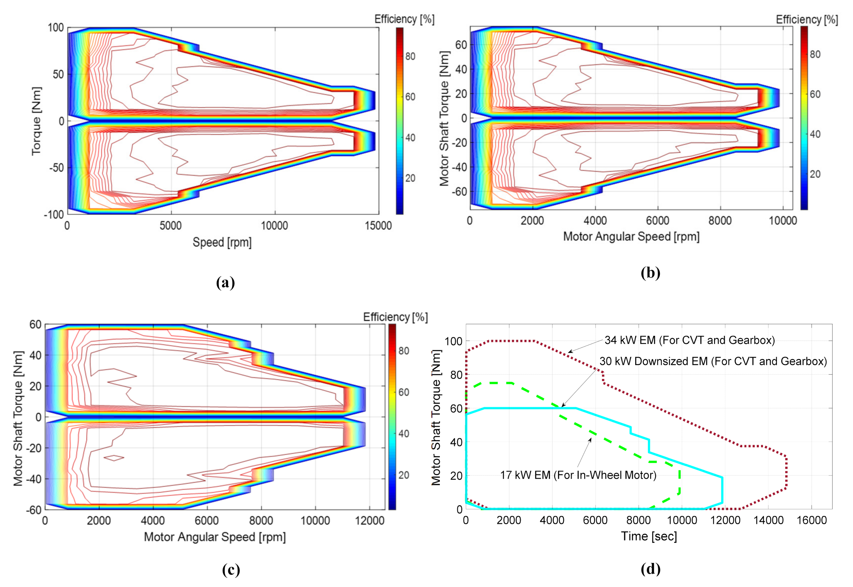
4. Model of Electric Motors and Concurrent Efficiency Maps

All the selected electric motors were a DC permanent magnet (PM) type, and their characteristics are expressed in the Appendix A section. For the in-wheel electric motor architecture, each of the in-wheel motor powers equaled 17 kW, and the total power of the vehicle was determined as 68 kW. On the other hand, for the architectures of 1G, 2G, and CVT, the motors had a separate power of 34 kW, and the total powers of the vehicles were the same for all the architectures. However, the power of the downsized electric motor was 30 kW, and the total power of the vehicle was 60 kW, less than that of the other architectures. The equations of the consumed and recovered currents are expressed in Equation (15), and the energy consumption of the fuel cells was activated during the driving case, while the state of charge of the supercapacitor was run during braking conditions.

$$I=\left\{\begin{array}{cc}\frac{T{\omega }_{EM}}{\mu V_C},\hfill & drivingsituation\hfill \\ \frac{\mu T{\omega }_{EM}}{V_C},\hfill & brakesituation\hfill \end{array}\right.$$

(15)

Here, the term $I$ represents the consumed and recovered current, $T$ is the motor shaft torque, ${\omega }_{EM}$ represents the angular speed of the electric motor, $\mu$ denotes the efficiency of the electric motor with respect to the torque and angular speed, and $V_C$ indicates the boost converter voltage. The efficiency of the electric motor is expressed as follows:

$$\mu =100\frac{T{\omega }_{EM}}{T{\omega }_{EM}+P_0+k_e{T}^2+k_w{\omega }_{EM}{}^2}$$

(16)

where $P_0$ is the fixed power loss, $k_e$ represents the torque-dependent electrical loss coefficient, and $k_w$ is the speed-dependent iron loss coefficient.

$$T_{peak}=k_T{D}_{EM}^2{L}_{EM}$$

(17)

The peak torque value can be found using Equation (17), where $k_T$ is described as a torque constant, $D_{EM}$ is the diameter of the motor, and $L_{EM}$ denotes the length of the motor.

Note that, the motor shaft torque T and angular speed ${\omega }_{EM}$ are exposed to gear ratios and their efficiencies given in

Table 2. The specifications of the powertrain layouts.

Differential Ratio	${\tau }_{diff}$	1:4
Differential efficiency	${\eta }_{diff}$	0.9
Gear ratio of 1G	${\tau }_{1G}$	1:3.625
Gear efficiency of 1G	${\tau }_{1G}$	0.92
First gear ratio of 2G	${\tau }_{2G1}$	1:2.724
First gear efficiency of 2G	${\eta }_{2G1}$	0.92
Second gear ratio	${\tau }_{2G2}$	1:1.251
Second gear efficiency of 2G	${\eta }_{2G2}$	0.92
Minimum CVT speed ratio	${\tau }_{CVT,min}$	0.4
Maximum CVT speed ratio	${\tau }_{CVT,max}$	2.5
Maximum CVT efficiency	${\eta }_{CVT,max}$	0.96
Minimum CVT efficiency	${\eta }_{CVT,min}$	0.89

. The efficiency map of CVT is adopted from [24].

5. PEM Fuel Cell and Supercapacitor Model

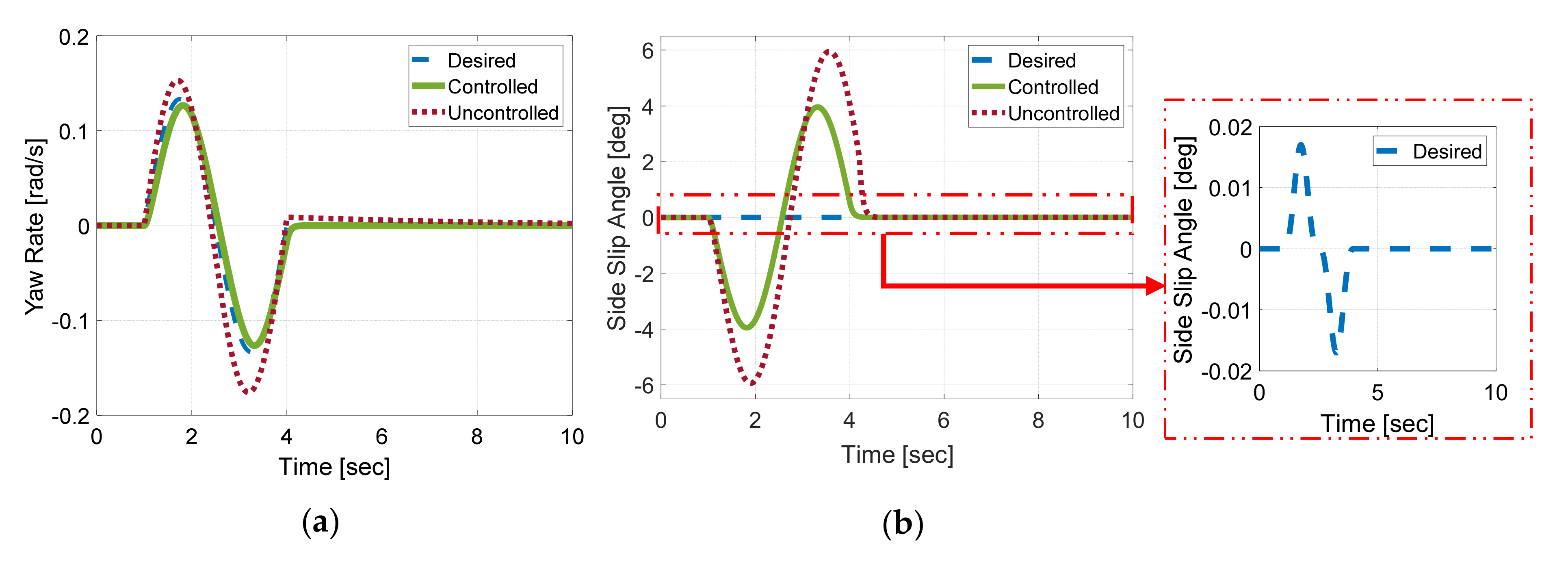
The referenced HFCEV had a 68 kW PEM fuel cell (PFC) and 7 kWh maximum stored energy supercapacitor as the two main energy sources. PEM fuel was considered the main energy source for the calculation of the energy consumption and supercapacitor for the energy recovery of the HFCEV. The characteristics of the fuel cell are presented in the Appendix A. The stack of PFCs had 255 cells. Each cell considered had the same efficiency. Equation (18) represents the Nernst equation for the voltage of one cell without energy losses.

$$V_{Nernst}=V_0+\frac{R{T}_{FC}}{2F}\ln \left(\frac{P_{H_2}{P}_{O_2}{}^{0.5}}{P_{H_{2}O}}\right)$$

(18)

Here, $V_0$ denotes an open-circuit voltage with a value equal to 1.2 V; $T_{FC}$ indicates the temperature of the PFC with a constant value of 50 °C. R is the universal gas constant; F is the Faraday constant; $P_{H_2}$, $P_{O_2}$, and $P_{H_{2}O}$ are the pressures of hydrogen gas, oxygen, and water vapor, respectively. The operating pressure of the fuel-cell system was set at a constant 1.5 bar. Equations (19)–(21) illustrate the voltage losses of the fuel cell in the order of the activation losses, $V_{act}$; concentration losses, $V_{con}$; and ohmic losses, $V_{\mathrm{ohm}}$, respectively. To simplify, the activation losses and concentration losses have been defined in the form of an empirical equation as a function of the current and temperature.

$$V_{act}=\frac{R{T}_{FC}}{n\alpha F}\ln (\frac{I}{I_0})$$

(19)

$$V_{con}=1.1\times {10}^{-4}-12\times {10}^{-6}\left(T_{FC}-273\right)e^{\left(0.008\right)I}$$

(20)

$$V_{\mathrm{ohm}}=\frac{t_m}{\sigma }I$$

(21)

where $I_0$ represents the referenced current, $\alpha$ is the transfer coefficient, $t_m$ denotes the membrane thickness with a value equal to 0.02 mm, and $\sigma$ denotes the electrical conductivity. The total voltage of the PFC $V_{FC}$ is presented in Equation (22) considering the voltage losses. Here, $N$ represents the stack number, and the fuel-cell unit had 255 cells.

$$V_{FC}=\left[V_{Nernst}-V_{act}-V_{con}-V_{ohm}\right]N$$

(22)

The fuel consumption of the PEM fuel cell, $HC$, was calculated using the linear function in Equation (23) based on the characteristics of the PFC.

$$HC=k_{FC}{V}_{FC}I$$

(23)

Here, $k_{FC}$ is the fuel consumption rate with respect to the power of the fuel cell, with a value equal to 0.01. By using Equation (24), it is possible to calculate the value of the charge voltage, $V_{sp}$, of the supercapacitor with respect to the recovered current during braking.

$$\frac{d{V}_{sp}}{dt}=\frac{1}{C}\frac{dQ}{dt}=\frac{1}{C_{sp}}I$$

(24)

Here, $C_{sp}$ represents the rated capacitance. The state of charge (SoC) rate of the supercapacitor was used for drawing a comparison of the energy recovery rates of the different architectures, according to Equation (25).

$$SoC=\%\frac{V_{sp}{}^2}{V_{sp,maks}{}^2}100$$

(25)

6. Results

In this section, the simulation results for the 14-degree-of-freedom (DoF) autonomous HFCEV model based on the regenerative electronic stability control strategy are demonstrated. To this end, the comparisons of the energy consumption and recovery performance of the six powertrain layouts, and the operation points of each electrical motor regarding the efficiency maps are illustrated. In addition, the vehicle handling performance of the RESC for four in-wheel electric motor architectures is presented. The characteristic profiles of the velocity, acceleration/deceleration, and power requirements for the FTP75 and NEDC drive cycles are shown in Figure 5.

Simulations of the RESC system were performed using 18 and 11 km-long double-lane-change maneuver paths for the FTP75 and NEDC urban drive cycles, respectively. Figure 6a shows the yaw rate performance, considering the double-lane-change maneuver, for comparing the RESC performance with the desired yaw rate and uncontrolled HFCEV. In addition, Figure 6b shows the sideslip angle performance with respect to the same maneuver for in-wheel layout with RESC. The obtained yaw rate with the RESC was within 7% of the desired value, while it is evident that the vehicle sideslip angle can be reduced. It can be concluded from this figure that the performance of the autonomous vehicle is satisfactory and the yaw rate is within 12% of the findings in [45]. After creating the illustrations of the RESC steering performance, the total and instant energy recovery performance of the rear in-wheel motors was calculated based on the double-lane-change maneuver using the RESC control strategy, as shown in Figure 7.

In order to determine the operation points of the electric motors in the efficiency map, the simulation results were plotted for FTP75 and NEDC, and these are illustrated in Figure 8. While the motor mode working points yielded approximately the same findings with and without RESC, different operation points were obtained for the generator mode due to the regenerative braking effect.

In Figure 9, the comparisons of the operation points of the electric motors for one-stage (1G), two-stage (2G), and CVT transmissions are presented. As shown in Figure 9a,b, the operation points shifted to the more efficient region, and the required torque was decreased significantly by using a transmission system. This achievement was due to a more flexible speed ratio, which allowed vehicles to run the electrical motors in more efficient operating regions.

Moreover, the mass, volume, and cost of the electric motors can also be reduced due to the decrease in the required peak torque. If the size of the electric motor is decreased, many more advantages can also be achieved, such as lower power losses and energy consumption, less cells in fuel cell stack, and lower total masses of the vehicles. Thus, in the study, the masses of the powertrain architecture were taken into account. A mass comparison between the vehicle architectures is given in Figure 10. It can be seen from this figure that the in-wheel motor layout has the lowest vehicle mass in comparison to the other designs; however, this architecture requires four independent motors, which increase the overall cost. On the other hand, the downsized electric motor layouts decrease the number of motors used and power electronic masses as well. Thus, the downsized layout is lighter than the two-stage transmission layout. Note that, two downsized electric motors were used and each of them was saved almost 10 kg mass. Additionally, since the power requirement of the fuel cell is decreased by using a downsized electric motor, it is also possible to have a lighter weight for the fuel cell. The simulations were repeated using the downsized electric motor, and the findings are illustrated in Figure 11.

Figure 12 illustrates the energy consumption performance of all six different types of EV for the NEDC and FTP75 drive cycles. It is evident that the consumption of in-wheel motors with RESC is less compared to that for the same construction without RESC; this is because energy is recovered in the RESC mode by the in-wheel motor. Moreover, the hydrogen fuel consumption rates with the CVT are better than with the one-stage and worse than with the two-stage gearbox, because a little extra energy is needed to operate the CVT. However, it should be noted that the downsized electric motor architecture shows the lowest consumption rates out of all the layouts owing to the CVT transmission, which allows the motor to work at the most efficient points. The state of charge (SoC) rates of the supercapacitor with respect to the NEDC and FTP75 drive cycles were also compared, and the results are presented in Figure 13. Based on these results, the downsized electric motor architecture recovers more energy than the other constructions.

The energy consumption and recovery rates per 100 km for all the different transmission units were also calculated, and these results are presented in Figure 14 and Figure 15, respectively. It can be seen that the downsized electric motor using a CVT yielded the lowest energy consumption rate and highest energy recovery rate. This is because, as emphasized earlier, the CVT allows the electric motor to operate in a more efficient zone. Additionally, it is noteworthy that an in-wheel motor architecture produces no transmission losses and that using an RESC system can increase the energy recovery percentage significantly.

Figure 16 illustrates the energy recovery/consumption rates, which are a valuable consideration in designing an efficient vehicle layout for each powertrain architecture. It is evident from this figure that the level of the energy recovery/consumption rate can significantly increase when using a downsized CVT. Additionally, it is apparent that the energy recovery/consumption rates increased with the use of an RESC system within an in-wheel-driven motor layout.

7. Conclusions

In this study, the energy consumption and recovery performance of six different powertrain architectures, including transmission and nontransmission layouts, were analyzed for HFCEVs. The stability control performance of RESC was tested with respect to the desired yaw rate and sideslip angle of the reference model, and the results were satisfactory. The conclusions of the study can be summarized as follows:

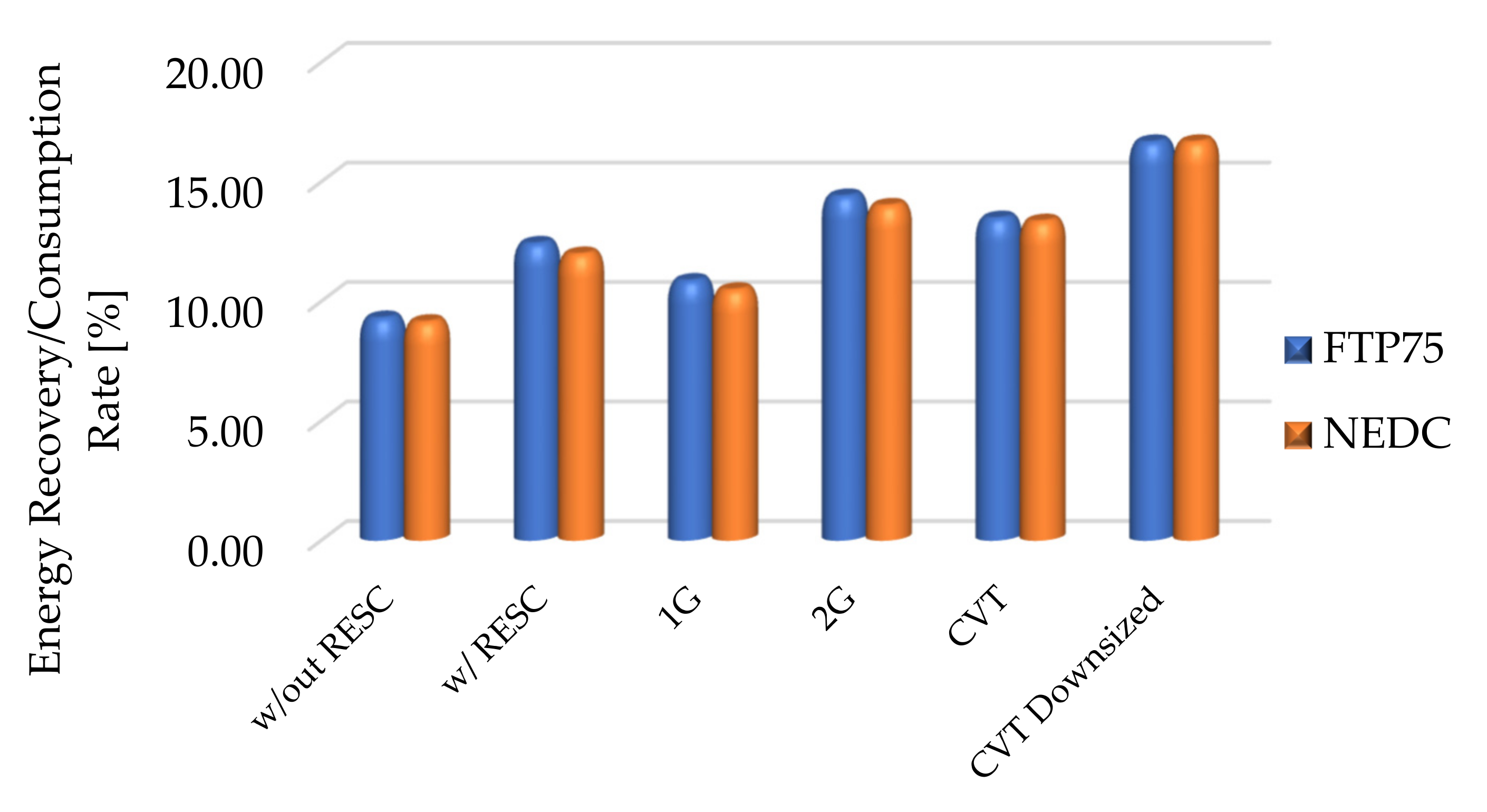
• A transmission system can reduce the energy consumption of HFCEVs tremendously as compared to other powertrain layouts, as it provides the optimum operating conditions for electric motors. If high torque capacity is required at low velocities of the vehicle, an automated transmission system must be used for improved energy consumption.
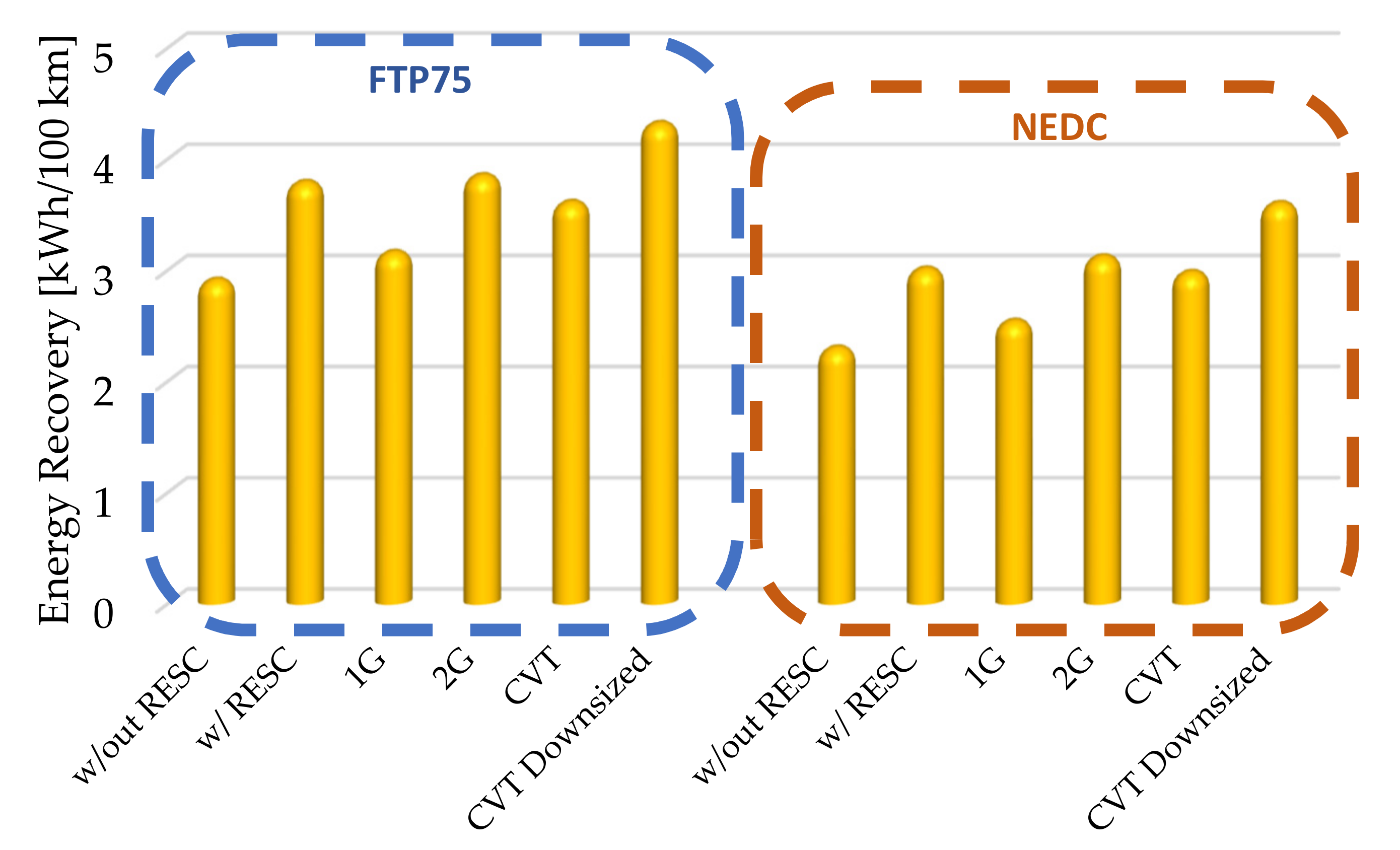
• An in-wheel motor layout is able to recover more energy if an RESC system is added to it. Overall, it spends less energy, except in the case of a downsized electric motor and two-stage automatic transmission. In addition, if the vehicle is used on a curved road, the in-wheel architecture with an RESC system can save a significant amount of energy.
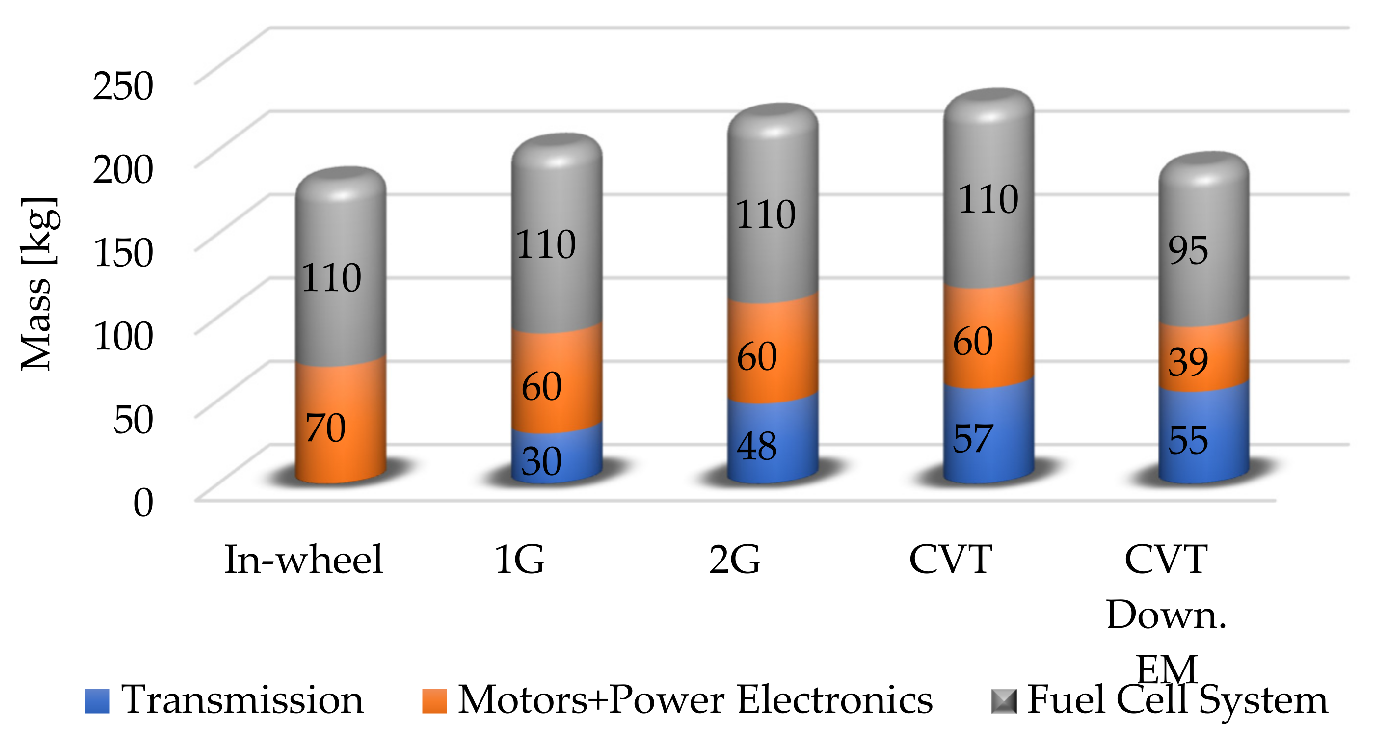
• Using a CVT transmission, the required peak torque of the electric motor can be decreased; therefore, it is possible to downsize the electric motor. Downsizing helps to achieve a reduction in the weight of not only the motor but also its driver and other power units, which results in the lowest energy consumption rate as compared to the other layouts.

The simulation results can be used for designing different types of vehicles, such as electric buses and trucks, as the findings will be easy to implement. Moreover, the simulation results can be further tested in future studies for exploring more innovations.

References

1. Kim, I.; Kim, J.; Lee, J. Dynamic analysis of well-to-wheel electric and hydrogen vehicles greenhouse gas emissions: Focusing on consumer preferences and power mix changes in South Korea. Appl. Energy 2020, 260, 114281. [Google Scholar] [CrossRef]
2. Wang, Q.; Xue, M.; Lin, B.; Lei, Z.; Zhang, Z. Well to wheel analysis of energy consumption, greenhouse gas and air pollutants emissions of hydrogen fuel cell vehicle in China. J. Clean. Prod. 2020, 275, 123061. [Google Scholar] [CrossRef]
3. Lathia, R.; Dobariya, K.; Patel, A. Hydrogen Fuel Cells for Road Vehicles. J. Clean. Prod. 2017, 141, 462. [Google Scholar] [CrossRef]
4. Ahmadi, P. Environmental impacts and behavioral drivers of deep decarbonization for transportation through electric vehicles. J. Clean. Prod. 2019, 225, 1209–1219. [Google Scholar] [CrossRef]
5. Xiong, H.; Liu, H.; Zhang, R.; Yu, L.; Zong, Z.; Zhang, M.; Li, Z. An energy matching method for battery electric vehicle and hydrogen fuel cell vehicle based on source energy consumption rate. Int. J. Hydrogen Energy 2019, 44–56, 29733–29742. [Google Scholar] [CrossRef]
6. Bartolozzi, I.; Rizzi, F.; Frey, M. Comparison between hydrogen and electric vehicles by life cycle assessment: A case study in Tuscany, Italy. Appl. Energy 2013, 101, 103–111. [Google Scholar] [CrossRef]
7. Grüger, F.; Dylewski, L.; Robinius, M.; Stolten, D. Carsharing with fuel cell vehicles: Sizing hydrogen refueling stations based on refueling behavior. Appl. Energy 2018, 228, 1540–1549. [Google Scholar] [CrossRef]
8. Wen, C.; Rogie, B.; Kaern, M.R.; Rothuizen, E. A first study of the potential of integrating an ejector in hydrogen fuelling stations for fuelling high pressure hydrogen vehicles. Appl. Energy 2020, 260, 113958. [Google Scholar] [CrossRef]
9. Cao, S.; Alanne, K. The techno-economic analysis of a hybrid zero-emission building system integrated with a commercial-scale zero-emission hydrogen vehicle. Appl. Energy 2018, 211, 639–661. [Google Scholar] [CrossRef]
10. Nagasawa, K.; Davidson, F.T.; Lloyd AC: Webber, M.E. Impacts of renewable hydrogen production from wind energy in electricity markets on potential hydrogen demand for light-duty vehicles. Appl. Energy 2019, 235, 1001–1016. [Google Scholar] [CrossRef]
11. Hoskins, A.L.; Milican, S.L.; Czernik, C.E.; Alshankiti, I.; Netter, J.C.; Wendelin, T.J.; Musgrave, C.B.; Weimer, A.W. Continuous on-sun solar thermochemical hydrogen production via an isothermal redox cycle. Appl. Energy 2019, 249, 368–376. [Google Scholar] [CrossRef]
12. Mastropasqua, L.; Pecenati, I.; Giostri, A.; Campanari, S. Solar hydrogen production: Techno-economic analysis of a parabolic dish-supported high-temperature electrolysis system. Appl. Energy 2020, 261, 114392. [Google Scholar] [CrossRef]
13. Eckert, J.; Silva, L.; Santiciolli, F.; Costa, E.; Corrêa, F.; Dedini, F. Energy storage and control optimization for an electric vehicle. Int. J. Energy Storage 2018, 42, 3506–3523. [Google Scholar] [CrossRef]
14. Hu, J.; Jiang, X.; Zheng, L. Design and analysis of hybrid electric vehicle powertrain configurations considering energy transformation. Int. J. Energy Storage 2018, 42, 4719–4729. [Google Scholar] [CrossRef]
15. Yang, X.; Taenaka, B.; Miller, T.; Snyder, K. Modeling validation of key life test for hybrid electric vehicle batteries. Int. J. Energy Storage 2010, 34, 171–181. [Google Scholar] [CrossRef]
16. Tie, S.F.; Tan, C.W. A review of energy sources and energy management system in electric vehicles. Renew. Sustain. Energy Rev. 2013, 20, 82–102. [Google Scholar] [CrossRef]
17. Changizian, S.; Ahmadi, P.; Raeesi, M.; Javani, N. Performance optimization of hybrid hydrogen fuel-cell electric vehicles in real driving cycles. Int. J. Hydrogen Energy 2020, 0360, 3199. [Google Scholar] [CrossRef]
18. Alamili, A.; Xue, Y.; Anayi, F. An experimental and analytical study of the ultra-capacitor storage unit used in regenerative braking systems. Energy Procedia 2019, 159, 376–381. [Google Scholar] [CrossRef]
19. Kaya, K.; Hames, Y. Two new control strategies: For hydrogen fuel saving and extending the life cycle in the hydrogen fuel cell vehicles. Int. J. Hydrogen Energy 2019, 44, 18967–18980. [Google Scholar] [CrossRef]
20. Tanç, B.; Arat, H.T.; Conker, Ç.; Baltacioğlu, E.; Aydin, K. Energy distribution analyses of an additional traction battery on hydrogen fuel cell hybrid electric vehicle. Int. J. Hydrogen Energy 2019, 45, 26344–26356. [Google Scholar] [CrossRef]
21. Ferreira, F.J.T.E.; Almeida, A.T. Induction motor downsizing as a low-cost strategy to save energy. J. Clean. Prod. 2012, 24, 117–131. [Google Scholar] [CrossRef]
22. De Pinto, S.; Camocardi, P.; Chatzikomis, C.; Sorniotti, A.; Bottiglione, F.; Mantriota, G.; Perlo, P. On the Comparison of 2- and 4-Wheel-Drive Electric Vehicle Layouts with Central Motors and Single- and 2-Speed Transmission Systems. Energies 2020, 13, 3328. [Google Scholar] [CrossRef]
23. Bottiglione, F.; De Pinto, S.; Mantriota, G.; Sorniotti, A. Energy consumption of a battery electric vehicle with infinitely variable transmission. Energies 2014, 7, 8317–8337. [Google Scholar] [CrossRef] [Green Version]
24. Sluis, F.; Romers, L.; Spijk GHupkes, I. CVT, promising solutions for electrification. SAE Int. Conf. Pap. 2019, 1, 0359. [Google Scholar] [CrossRef]
25. Liang, J.; Walker, P.D.; Ruan, J.; Yang, H.; Wu, J. Gear shift and brake distribution control for regenerative braking in electric vehicles with dual clutch transmission. Mech. Mach. Theory 2019, 133, 1–22. [Google Scholar] [CrossRef]
26. Mo, W.; Walker, P.D.; Fang, Y.; Wu, J.; Ruan, J.; Zhang, N. A novel shift control concept for multi-speed electric vehicles. Mech. Syst. Signal Process. 2018, 112, 171–193. [Google Scholar] [CrossRef]
27. Zhang, L.; Ca, X. Control strategy of regenetrative braking system in electric vehicles. Energy Procedia 2018, 152, 496–501. [Google Scholar] [CrossRef]
28. Ruan, J.; Walker, P.; Zhang, N. A comparative study energy consumption and costs of battery electric vehicle transmissions. Appl. Energy 2016, 165, 119–134. [Google Scholar] [CrossRef] [Green Version]
29. Yildiz, A.; Kopmaz, O.; Cetin, S.T. Dynamic modeling and analysis of a four-bar mechanism coupled with a CVT for obtaining variable input speeds. J. Mech. Sci. Technol. 2015, 29, 1001–1006. [Google Scholar] [CrossRef]
30. Yildiz, A.; Piccininni, A.; Bottiglione, F.; Carbone, G. Modeling chain continuously variable transmission for direct implementation in transmission control. Mech. Mach. Theory 2016, 105, 428–440. [Google Scholar] [CrossRef]
31. Yildiz, A.; Bottiglione, F.; Carbone, G. An experimental study on the shifting dynamics of the chain CVT. Int. Conf. Adv. Mech. Robot. Eng. 2015. [Google Scholar] [CrossRef]
32. Yildiz, A.; Kopmaz, O. Control-oriented modelling with experimental verification and design of the appropriate gains of a PI speed ratio controller of chain CVTs. Stroj. Vestn. J. Mech. Eng. 2017, 63, 374–382. [Google Scholar] [CrossRef] [Green Version]
33. Yildiz, A.; Bottiglione, F.; Piccininni, A.; Kopmaz, O.; Carbone, G. Experimental validation of the Carbone–Mangialardi–Mantriota model of continuously variable transmission. Proc. Inst. Mech. Eng. Part D J. Automob. Eng. 2018, 232. [Google Scholar] [CrossRef]
34. Yildiz, A.; Kopmaz, O. Dynamic analysis of a mechanical press equipped with a half-toroidal continuously variable transmission. Int. J. Mater. Product Technol. 2015, 50, 22–36. [Google Scholar] [CrossRef]
35. Arango, I.; Muñoz Alzate, S. Numerical Design Method for CVT Supported in Standard Variable Speed Rubber V-Belts. Appl. Sci. 2020, 10, 6238. [Google Scholar] [CrossRef]
36. Wang, Z.; Cai, Y.; Zeng, Y.; Yu, J. Multi-Objective Optimization for Plug-In 4WD Hybrid Electric Vehicle Powertrain. Appl. Sci. 2019, 9, 4068. [Google Scholar] [CrossRef] [Green Version]
37. Li, H.; Zhou, Y.; Xiong, H.; Fu, B.; Huang, Z. Real-Time Control Strategy for CVT-Based Hybrid Electric Vehicles Considering Drivability Constraints. Appl. Sci. 2019, 9, 2074. [Google Scholar] [CrossRef] [Green Version]
38. Mingyao, Y.; Datong, Q.; Xingyu, Z.; Sen, Z.; Yuping, Z. Integrated optimal control of transmission ratio and power split ratio for a CVT-based plug-in hybrid electric vehicle. Mech. Mach. Theory 2019, 136, 52–71. [Google Scholar] [CrossRef]
39. Jain, M.; Williamson, S.S. Suitability analysis of in-wheel motor direct drives for electric and hybrid electric vehicles. IEEE Electr. Power Energy Conf. 2019, 988, 1–5. [Google Scholar] [CrossRef]
40. Long, G.; Ding, F.; Zhang, N.; Zhang, J.; Qin, A. Regenerative active suspension system with residual energy for in-wheel motor driven electric vehicle. Appl. Energy 2020, 260, 114180. [Google Scholar] [CrossRef]
41. Kulkarni, A.; Ranjha, S.A.; Kapoor, A. Fatigue analysis of a suspension for an in-wheel electric vehicle. Eng. Fail. Anal. 2016, 68, 150–158. [Google Scholar] [CrossRef]
42. Najjari, B.; Mirzae, M.; Tahouni, A. Constrained stability control with optimal power management strategy for in-wheel electric vehicles. J. Multi-Body Dyn. 2019, 1–19. [Google Scholar] [CrossRef]
43. Xu, W.; Chen, H.; Zhao, H.; Ren, B. Torque optimization control for electric vehicles with four in-wheel motors equipped with regenerative braking system. Mechatronics 2019, 57, 95–108. [Google Scholar] [CrossRef]
44. Ehsani, M.; Gao, Y.; Gay, S.E.; Emadi, A. Modern Electric, Hybrid Electric, and Fuel Cell Vehicles Fundamentals, Theory, and Design; CRC Press: Boca Raton, FL, USA, 2005; ISBN 0-8493-3154-4. [Google Scholar]
45. Tekin, G.; Unlusoy, Y.S. Design and simulation of an integrated active yaw control system for road vehicles. Int. J. Veh. Des. 2010, 52. [Google Scholar] [CrossRef]
Figure 1. Block diagram of the developed model.
Applsci 11 02515 g001
Figure 2. (a) Vehicle architectures electric vehicles (EV); (b) energy supply diagram of hydrogen fuel-cell electric vehicle (HFCEV).
Applsci 11 02515 g002
Figure 3. Vehicle dynamic model: (a) Top view; (b) Back view.
Applsci 11 02515 g003
Figure 4. Yaw rate controller scheme.
Applsci 11 02515 g004
Figure 5. Characteristic profiles of the velocity (a), acceleration/deceleration (b), and power requirements (c) of the FTP75 and NEDC.
Applsci 11 02515 g005
Figure 6. Comparison of regenerative electronic stability control (RESC), (a) with respect to yaw rates and (b) from sideslip angle for in-wheel layout with RESC.
Applsci 11 02515 g006
Figure 7. Total and instant energy recovery during regenerative stability control.
Applsci 11 02515 g007
Figure 8. In-wheel motor with and without regenerative electronic stability control (RESC) for (a) the FTP75 and (b) NEDC.
Applsci 11 02515 g008
Figure 9. Operation points of the EV equipped with one-stage (1G), two-stage (2G), and CVT transmission for (a) the FTP75 and (b) NEDC.
Applsci 11 02515 g009
Figure 10. Comparison of the main subsystem masses.
Applsci 11 02515 g010
Figure 11. Downsized CVT operation points for (a) the FTP75 and (b) NEDC.
Applsci 11 02515 g011
Figure 12. Comparison of the consumed hydrogen: (a) FTP75 drive cycle; (b) NEDC drive cycle.
Applsci 11 02515 g012
Figure 13. Comparison of energy recovery: (a) FTP75 drive cycle; (b) NEDC drive cycle.
Applsci 11 02515 g013
Figure 14. Energy consumption rates per 100 km for FTP75 and NEDC.
Applsci 11 02515 g014
Figure 15. Energy recovery rates per 100 km for FTP75 and NEDC.
Applsci 11 02515 g015
Figure 16. Comparison of energy recovery/consumption rates.
Applsci 11 02515 g016