An Overview of Hybrid RANS–LES Models Developed for Industrial CFD

Abstract

An overview of scale-resolving simulation (SRS) methods used in ANSYS Computational Fluid Dynamics (CFD) software is provided. The main challenges, especially when computing boundary layers in large eddy simulation (LES) mode, will be discussed. The different strategies for handling wall-bound flows using combinations of RANS and LES models will be explained, along with some specific application examples. It will be demonstrated that the stress-blended eddy simulation (SBES) approach is optimal for applications with a mix of boundary layers and free shear flows due to its low cost and its ability to handle boundary layers in both RANS and wall-modeled LES (WMLES) modes.

1. Introduction

Historically, industrial Computational Fluid Dynamics (CFD) simulations have been based on Reynolds-averaged Navier–Stokes (RANS) turbulence modeling concepts. While computationally efficient, RANS models cannot always provide the degree of accuracy or the level of (unsteady) information required during the design process. Since the resolution of the entire turbulent spectrum in the entire flow domain using direct numerical simulations (DNS) techniques is insufficient, divide-and-conquer strategies are employed. This means that only parts of the turbulent spectrum are resolved, or the turbulence is only resolved in a part of the computational domain. Such methods are termed scale-resolving simulation (SRS) methods in this article.

Classical examples in which RANS cannot provide all of the necessary information are aero-acoustics simulations, whereby the turbulence generates noise sources that cannot be extracted accurately from RANS simulations. Other examples are flows with unsteady heat-loading due to flow streams of different temperatures, which can lead to material failure, or multi-physics effects such as vortex cavitation, in which the unsteady turbulence pressure field is the cause of cavitation. In such situations, the need for SRS can exist, even when a RANS model would in principle be capable of computing the correct time-averaged flow field.

The second reason for using SRS models is accuracy. RANS models have shown their strength for wall-bound flows, whereby the calibration according to the law-of-the-wall provides a sound foundation for further refinement. For free shear flows, the performance of RANS models is much less uniform. There is a wide variety of such flows, ranging from simple self-similar flows such as jets, mixing layers, and wakes to impinging flows, flows with strong swirls, massively separated flows, and many more. Considering that RANS models typically already have limitations covering the most basic self-similar free shear flows with one set of constants, there is little hope that even the most advanced Reynolds stress models (RSM) will eventually be able to provide a reliable foundation for all such flows. For an overview of RANS modeling and its limitations, see Durbin et al. [1], Wilcox [2], Hanjalic and Launder [3], and Bush et al. [4].

For free shear flows, it is often feasible to resolve the largest turbulence scales, as they are of the order of the shear layer thickness. In contrast, in wall boundary layers, the turbulent length scale near the wall becomes very small relative to the boundary layer thickness (increasingly so at higher Re numbers). This poses severe limitations for large eddy simulations (LES), as the computational effort required is still far from the computing power available to the industry (e.g., Spalart [5]). For an overview of LES modeling and its resource requirements, see Sagaut [6] and Guerts [7]. For this reason, hybrid models are increasingly applied, whereby large eddies are resolved away from walls and the wall boundary layers are covered by a RANS model. Examples of such global hybrid models are detached eddy simulation (DES) (Spalart, [8], Strelets [9], Travin et al. [10]), scale-adaptive simulation (SAS) (Menter and Egorov [11] and Egorov et al. [12]), and Partially Averaged Navier–Stokes (PANS) models (Girimaji et al. [13,14]). More advanced versions of DES include delayed DES (DDES), shear-layer-adapted (SLA) DDES (DDES-SLA), and improved DDES (IDDES) (Shur et al. [15], Spalart et al. [16], Shur et al. [17], Gritskevich [18]). More recent developments are the shielded detached eddy simulation (SDES) and the stress-blended eddy simulation (SBES) models (Menter [19]).

A further step is to apply a RANS model only in the innermost part of the wall boundary layer and then to switch to a LES model for the main part of the boundary layer. Such models are termed wall-modeled LES (WMLES) models (e.g., Shur et al. [15]). Finally, for large domains, it is frequently necessary to cover only a small portion with SRS models, while most of the flow can be computed in RANS mode. In such situations, zonal or embedded LES (ELES) methods are attractive, as they allow one to explicitly specify the region where LES is required (e.g., Cokljat et al. [20], Deck et al. [21] Xiao [22]). Such methods are typically not new models in the strict sense but allow the combination of existing models or technologies in a flexible way in different portions of the flow field. Important elements of zonal models are interface conditions, which convert turbulence from RANS mode to resolved mode. In most cases, this is achieved by introducing synthetic turbulence based on the length and time scales from the RANS model (e.g., Shur et al. [23]).

There are many hybrid RANS–LES models, often with somewhat confusing naming conventions, which vary in the strategy of how they split up the domain into RANS and LES regions. For a general overview of SRS modeling concepts, see Fröhlich and von Terzi [24], Sagaut et al. [25], and Chaouat [26], or the Scale-Resolving Simulation (SRS) Best Practice document by Menter [27].

Unfortunately, there is no unique model covering all industrial flows, and each individual model poses its own set of challenges. In general, the CFD practitioner must understand the intricacies of the SRS model formulation to be able to select the optimal model and to use it efficiently. This article is intended to enhance the basic understanding of such models. The discussion is naturally focused on the models available in the ANSYS CFD software. Some details of these models are unpublished. In these cases, the underlying ideas and concepts are described as far as possible, so that the reader can relate these methods to other public domain formulations. All simulations were conducted with ANSYS Fluent^®, a generalized, commercial finite-volume CFD code solving flows in structured and unstructured meshes.

2. Large Eddy Simulation of Wall-Bound Flows

To understand the motivation for the use of hybrid models, one must discuss the limitations of LES. LES has been the most widely explored SRS model over recent decades. It is based on the concept of resolving only large scales of turbulence and modeling the small scales. The classical motivation for LES is that the large scales are problem-dependent and difficult to model, whereas the smaller scales are more universal and isotropic and can be modeled more easily.

LES is based on filtering the Navier–Stokes equations over a finite spatial region (typically the grid volume) and is aimed at only resolving the portions of turbulence larger than the filter width. Turbulence structures smaller than the filter are then modeled—typically using a simple eddy viscosity model.

It is generally agreed that LES eddy viscosity models only model dissipation, not the physics of the feedback from small and large scales (“backscatter”). As a result, within the LES framework, all features and effects of the flow that are of interest and relevant to engineers must be resolved in space and time. This makes LES a very CPU-expensive technology.

Most demanding is the application of LES to wall-bound flows. In the logarithmic near-wall layer, the turbulent length scale, L_t, of the large eddies can be expressed as:

$${\mathrm{L}}_t=\kappa y$$

(1)

where y is the wall distance and κ is a constant. In other words, even the (locally) largest scales become very small near the wall and require a high resolution in all three space dimensions and in time.

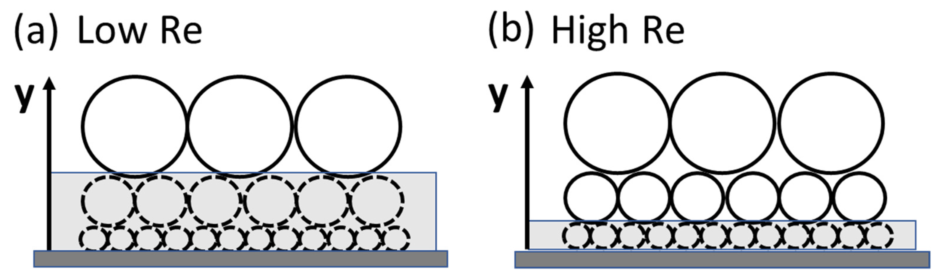
The linear dependence of L_t on y indicates that the turbulence length scales approach zero near the wall, meaning an infinitely fine grid would be required to resolve them. However, this is not the case, as the molecular viscosity prevents scales smaller than the Kolmogorov limit. This is manifested by the viscous or laminar sublayer, a region very close to the wall, where small-scale turbulence is damped and does not need to be resolved. However, the viscous sublayer thickness is a function of the Reynolds number, Re, of the flow. At higher Re numbers, the viscous sublayer becomes thinner, thereby allowing the “survival” of smaller eddies that need to be resolved. This is depicted in Figure 1, showing a sketch of turbulence structures in the vicinity of the wall (e.g., channel flow with the flow direction oriented toward the observer). The left part of the picture represents a situation with a low Re number with the right part shows situation with a higher Re number. The grey box indicates the viscous sublayer for the two Re numbers. The structures inside the viscous sublayer (circles inside the grey box) are depicted but not active due to viscous damping. Only the structures outside of the viscous sublayer (i.e., above the grey box) exist and need to be resolved. Due to the reduced thickness of the viscous sublayer in the high Re case, substantially more resolution is required to resolve all active scales. The Wall-Resolved LES (WRLES) approach is, therefore, prohibitively expensive for moderate to high Reynolds numbers. This is the main reason why WRLES is not suitable for most engineering flows.

The Reynolds number scaling can be reduced by the application of Wall Functions (WFLES) with ever increasing y+ values for higher Re numbers. There has been a renewed interest in recent years in advanced wall functions (e.g., Bae et al. [28], Cho et al. [29], Kawai et al. [30], and Lozano-Duran [31]). In principle, the application of WFLES allows the resolution of a boundary layer volume using a constant number of cells, independent of the Reynolds number.

The final alternative to WRLES and WFLES is the Wall-Modeled LES (WMLES) approach. In this approach, the stream- and spanwise resolution are identical to those in a WFLES grid, however the wall-normal direction can be resolved through the viscous sublayer. This is achieved by blending a RANS model near the wall with a LES model away from the wall. The switch takes place in the logarithmic layer. WMLES can either be achieved by using a transport-equation-based model (IDDES, SBES) or an algebraic (Prandtl mixing length) model in the inner layer (Shur et al. [23].

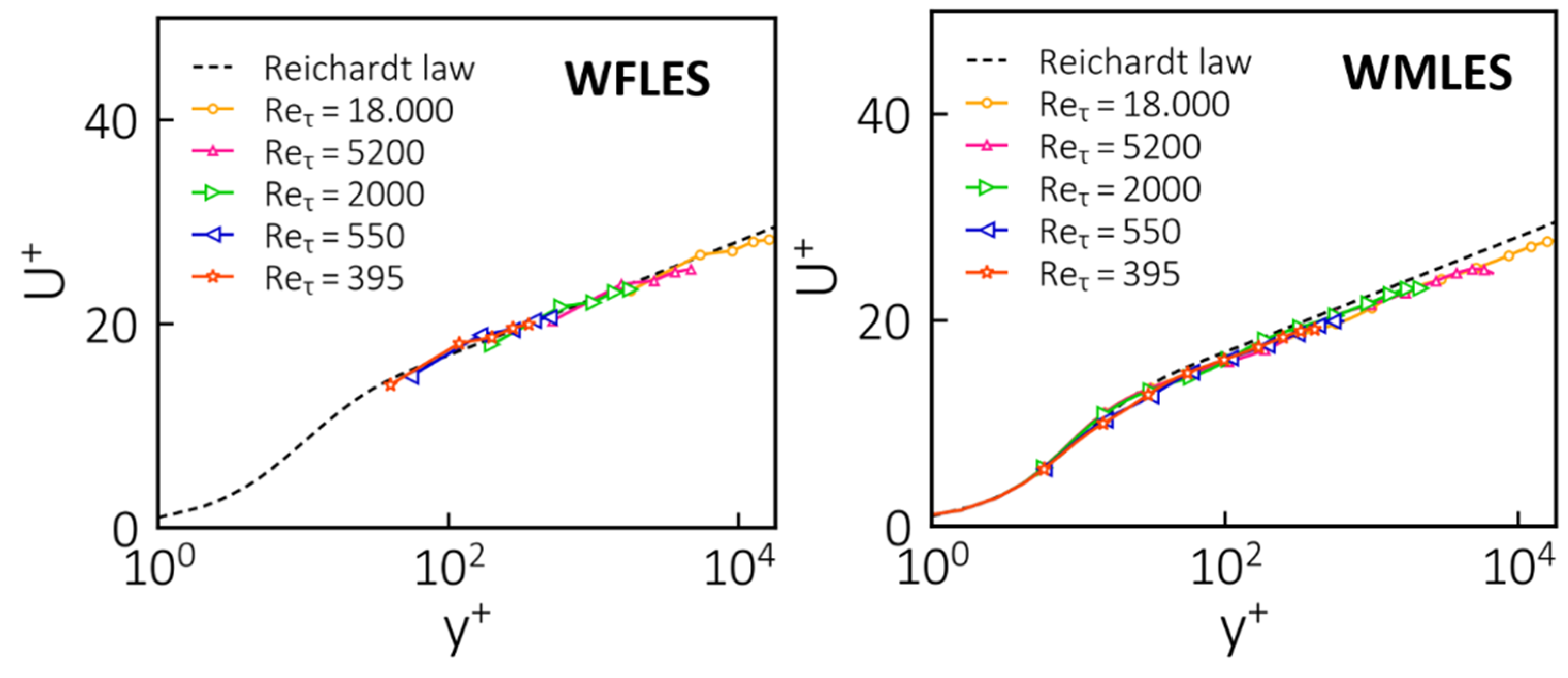
Figure 2 shows the results of WFLES and WMLES approaches for channel flows with different $R{e}_{\tau }=\frac{u_{\tau }H/2}{\nu }$ numbers, using a grid of around 5 × 10⁵ cells for all Re numbers ($u_{\tau }$ = friction velocity, H = channel height, and ν = kinematic viscosity). Both methods provide a good representation of the expected linear–logarithmic correlations. It is interesting to note that the current WFLES implementation avoids the well-known log–layer mismatch when applying a wall function in the center of the first cell. This is achieved through careful computation of velocity gradients in this cell.

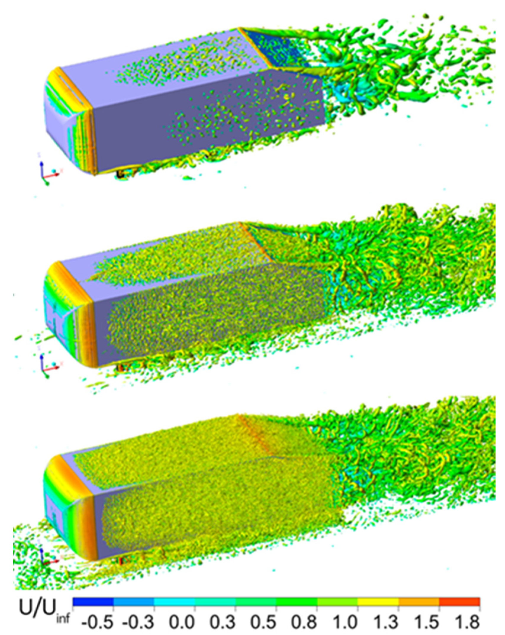
The application of the WFLES approach in external automotive applications has received increased attention, at least for models involving reduced Re numbers (e.g., Ambo et al. [32]). A classical starting point for validation of methods for such applications is the Ahmed car body approach, a strongly simplified geometry involving the main features of a hatchback car. WFLES simulations were carried out for a 25° slant angle case. Three octree meshes with different grid sizes (mesh 1 = 7 × 10⁶; mesh 2 = 35 × 10⁶; mesh 3 = 100 × 10⁶) were used. Resolved turbulent flow structures can be seen in Figure 3, with a clear increase in detail under mesh refinement conditions.

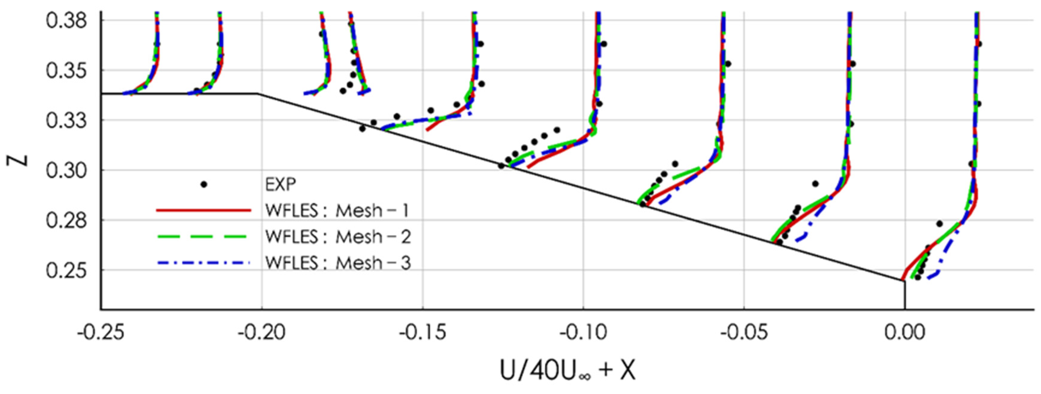
Figure 4 shows the resulting velocity profiles in the critical region above the slant. This region is characterized in the experiments by a closed separation bubble from the slant onset halfway down the slant. The WFLES solutions provide a reasonable agreement with the experimental data in the study by Lienhart and Becker [33], albeit not with the same detail. All WFLES solutions tend to predict an acceleration at the slant onset that is not seen in the experiment. This seems to be caused by a lack of wall-normal resolution in the WF grids near the geometric singularity at the slant onset. As a result of this acceleration, the flow exhibits a reduced separation tendency downstream of the slant. With mesh refinement, the flow also accelerates too strongly towards the end of the slant.

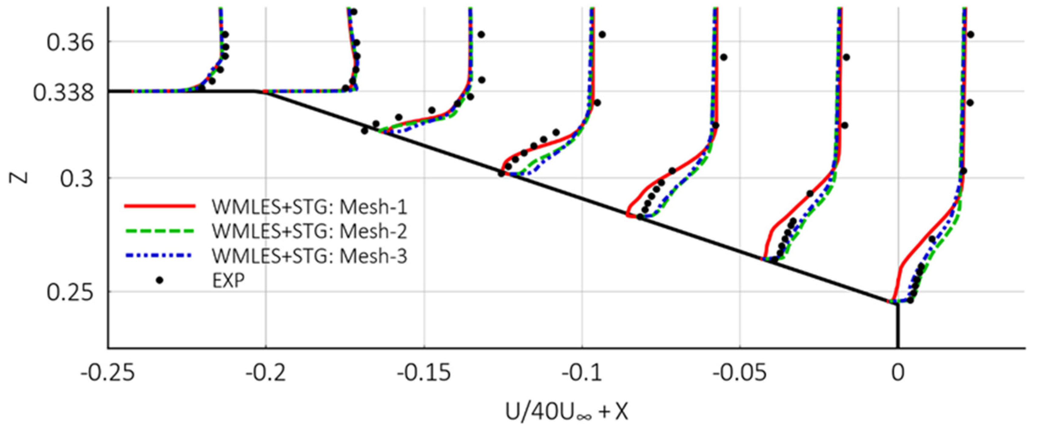
WMLES were performed on the same geometry, using y + ~1 meshes of a different size (mesh 1 = 10 × 10⁶; mesh 2 = 20 × 10⁶; mesh 3 = 40 × 10⁶) in the slant region. As can be seen in Figure 5, in these meshes, the acceleration around the slant is avoided, pointing to an advantage of this approach over WFLES, due to the finer wall-normal resolution. The agreement with the experiment is generally improved relative to the WFLES results, but again shows a tendency towards reduced separation size downstream of the slant onset, especially for the finer meshes. Note that this case is notoriously difficult to compute with LES (at least at the experimental Re number), as seen in a comparative study by Serre et al. [34], whereby different groups produced solutions ranging from fully stalled to non-separated. Similarly to the findings of Serre et al., it is concluded that much finer meshes would be required to achieve mesh-independent solutions for this case when covering the boundary layer in any form of LES. Simulations using a hybrid RANS–LES method for this case will be discussed in the next section.

The results for both WFLES and WMLES show that it is challenging to achieve grid-converged solutions with such methods, even for semi-realistic flows. This is the motivation for the development of hybrid RANS–LES methods, which utilize well-calibrated RANS techniques in the boundary layers.

3. Global Hybrid RANS–LES Models

Many hybrid RANS–LES methods have been developed in the last two decades, following the original proposal by Spalart [8]. From an industrial standpoint, mostly models of the DES family, and in the case of ANSYS the SAS (e.g., Menter and Egorov [11], Egorov et al. [12]) and SBES models (Menter [19]), have had wider impacts. Since the introduction of the SBES model, it has essentially replaced the older hybrid models in ANSYS and is now widely used in many applications (see Ekman et al. [35], Pergande and Abdel-Maksoud [36], Kim and Chang [37]).

The SBES model is considered by the current authors as “optimal”, as it satisfies the following properties:

• It is a building block method, allowing existing RANS and LES methods to be combined;
• Allows asymptotic shielding of the RANS boundary layer under mesh refinement;
• Provides an optimal “transition” from RANS to LES;
• Can operate in WMLES mode;
• Is low cost.

The SBES model is based on the blending of existing RANS and LES models using:

$${\mathsf{\tau }}_{\mathrm{ij}}^{\mathrm{SBES}}={\mathrm{f}}_{\mathrm{SBES}}\cdot {\mathsf{\tau }}_{\mathrm{ij}}^{\mathrm{RANS}}+\left(1-{\mathrm{f}}_{\mathrm{SBES}}\right)\cdot {\mathsf{\tau }}_{\mathrm{ij}}^{\mathrm{LES}}$$

(2)

where ${\mathsf{\tau }}_{\mathrm{ij}}^{\mathrm{RANS}}$ is the RANS part and ${\mathsf{\tau }}_{\mathrm{ij}}^{\mathrm{LES}}$ the LES part of the modeled stress tensor. If both model portions are based on eddy viscosity concepts, the formulation simplifies to a blend of the eddy viscosities:

$${\mathsf{\nu }}_{\mathrm{t}}^{\mathrm{SBES}}={\mathrm{f}}_{\mathrm{SBES}}\cdot {\mathsf{\nu }}_{\mathrm{t}}^{\mathrm{RANS}}+\left(1-{\mathrm{f}}_{\mathrm{SBES}}\right)\cdot {\mathsf{\nu }}_{\mathrm{t}}^{\mathrm{LES}}$$

(3)

The key element is the blending function f_SBES, which is f_SBES = 1 inside boundary layers and f_SBES = 0 for separated and free shear flows. It is essential that the function remains at f_SBES = 1 inside boundary layers to shield the boundary layer from any impact from the LES model. Premature switching to the LES model inside the boundary layer would result in failure.

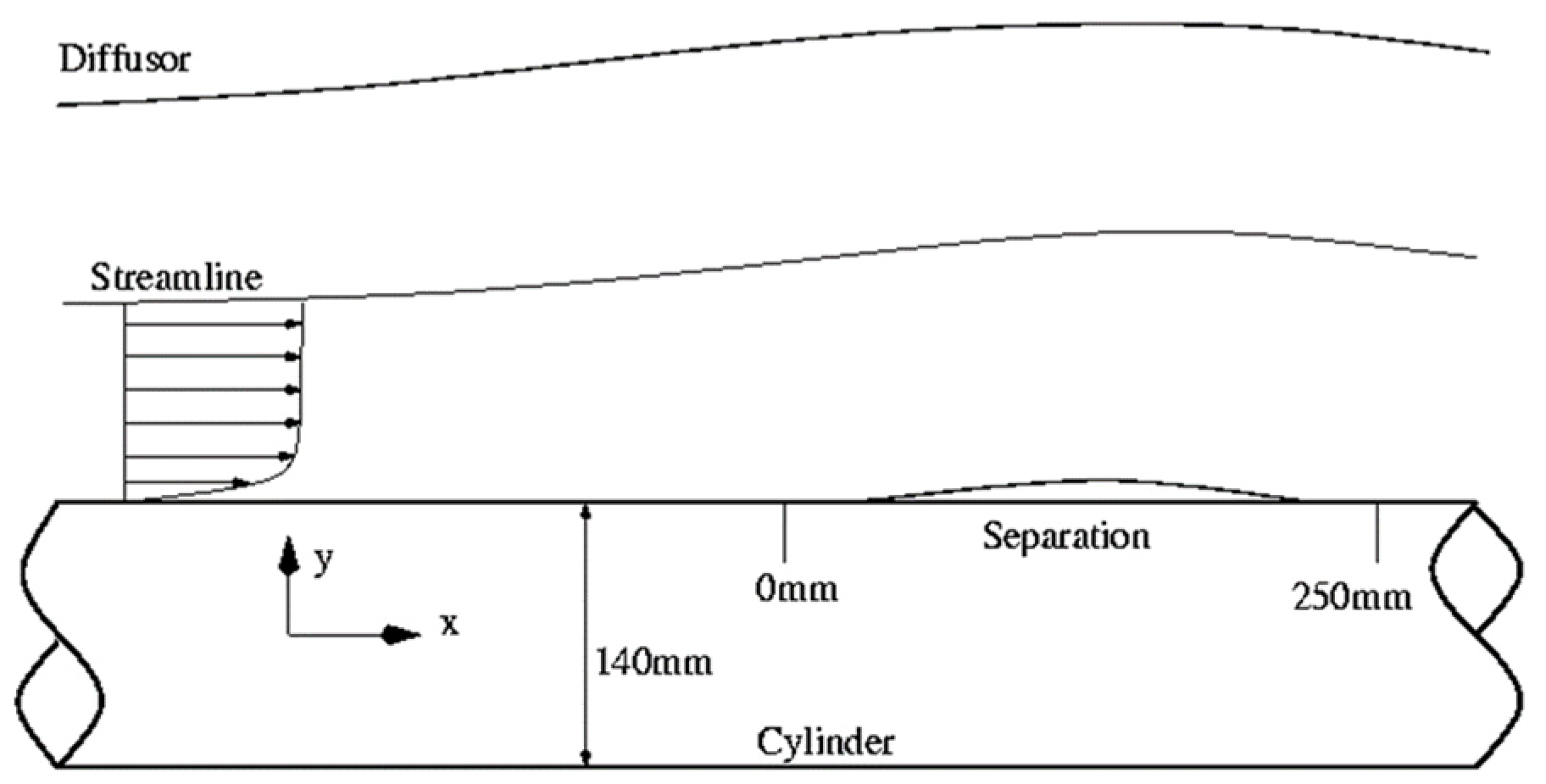
This can be demonstrated for a diffuser flow, as shown in Figure 6. In this test case, the boundary layer flows in the axial direction of the inner cylinder. A pressure gradient is imposed by an outwards expanding slip wall. The pressure gradient results in significant thickening of the boundary layer. The purpose of this test is not to demonstrate the accuracy of the RANS models, but to show the behavior of different shielding functions and their impacts on the eddy viscosity distribution inside the boundary layer.

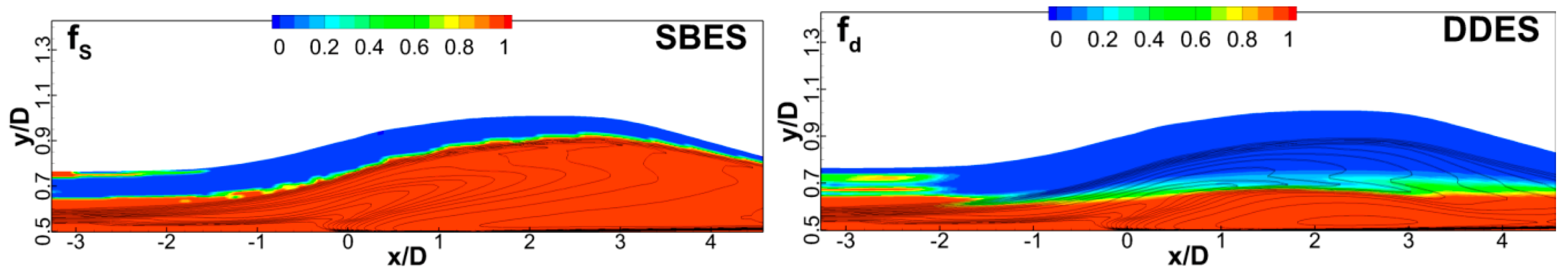
Figure 7 shows the comparison of SBES and DDES shielding functions for the diffuser flow. The SBES shielding covers the entire boundary layer, including the rapid growth area due to the separation bubble, while DDES preserves only the thin boundary layer near the inlet. This means that in the adverse pressure gradient region, the shielding properties of DDES are substantially impaired for this case.

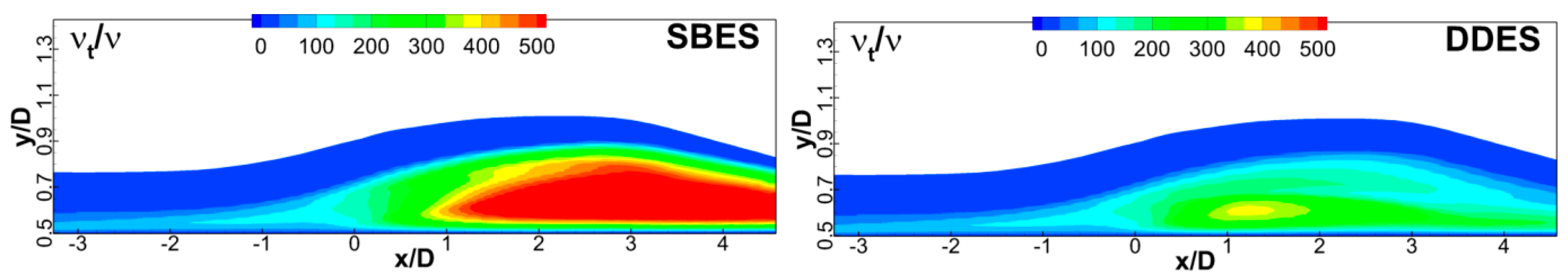
This has consequences for the eddy viscosity fields shown in Figure 8. The ratio of the eddy viscosity to molecular viscosity for the SBES approach corresponds to the ratio for the SST model, while the DDES model produces much reduced levels in the adverse pressure gradient region. This can lead to grid-induced separation (GIS), a highly undesirable situation, whereby grid refinement leads to artificial separations (Menter and Kuntz [38]).

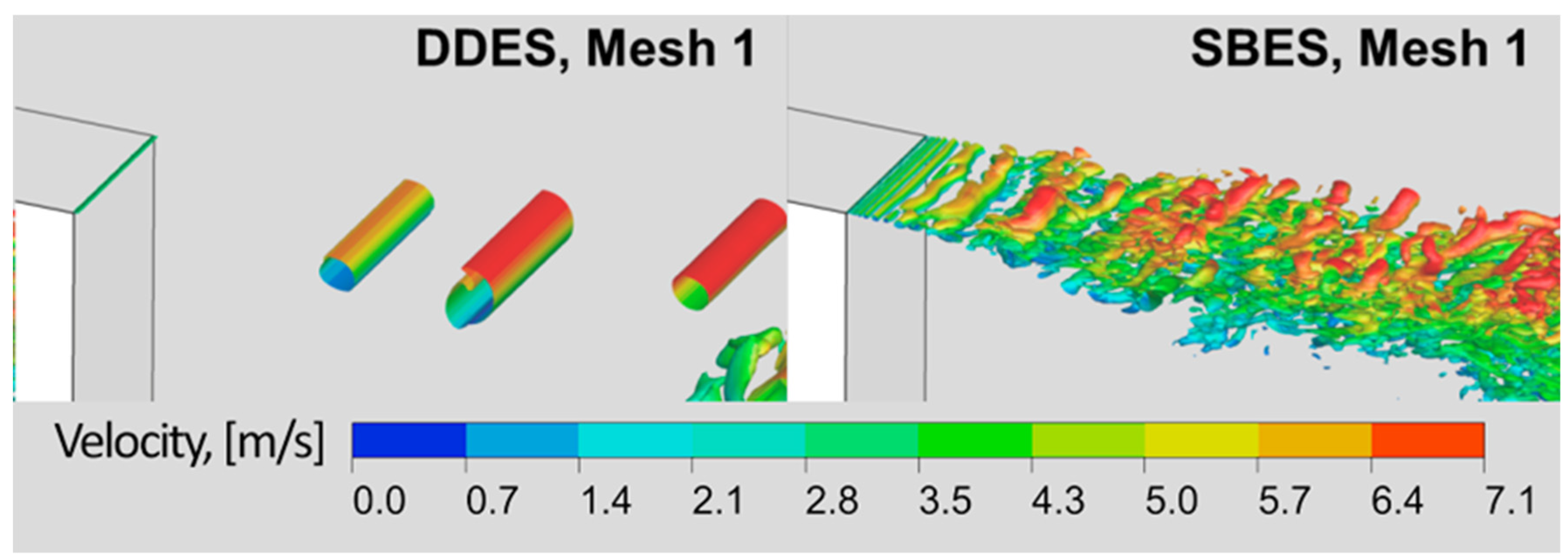
The RANS–LES transition is an artificial process that occurs in the region where the hybrid model switches from RANS mode to LES mode. In this process, the upstream RANS turbulence content is lost, as the RANS model is essentially turned off, while no resolved LES content is yet available. To preserve the consistency of the simulation, it is essential that the resolved turbulence is created as quickly as possible in order to achieve a balanced flow field. This “transition” process depends on many details, such as the grid resolution, the numerical dissipation, and the details of the hybrid model. Since the SBES model switches sharply from RANS to an existing algebraic LES model, the “grey zone” of the intermediate RANS–LES eddy viscosities is avoided and resolved turbulence can form quickly. This can be seen for the mixing layer (Morris and Foss [39]) shown in Figure 9, where the SBES model develops fine-grained turbulence, while the DDES approach maintains 2D structures in the same grid of 2 × 10⁶ cells. More modern DES versions such as DDES–SLA [17] also help to reduce the delay of resolved structures.

The CPU cost for SBES can be minimized by recognizing that the RANS part of the flow typically follows a slower time scale than the LES part. It is, therefore, possible to update the two-equation RANS model part with a larger time step than the cheaper LES model. Updating the RANS part at only every 3rd to 5th time step leads to a decrease of around 20% in the overall computational time. The cost per time step for the SBES is then only marginally higher than for a pure LES model on the same mesh.

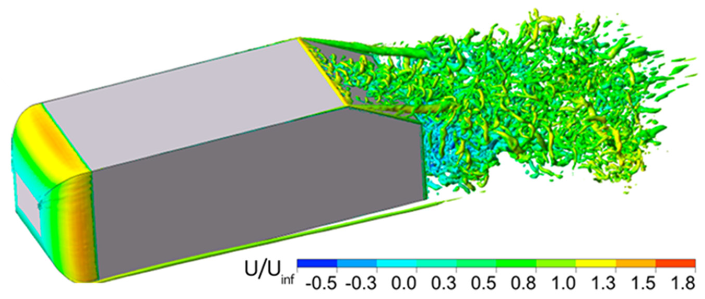
To demonstrate the capabilities of SBES, the Ahmed car body at 25° was computed with the SBES model using a combination of the SST–RANS and the WALE–LES models. The flow conditions are taken from the experiment by Lienhart and Becker [33], with a Reynolds number based on a car height of Re_H = 7.68 × 10⁵. The simulation was carried out on a moderate 14 × 10⁶-cell hex grid. Figure 10 shows the resolved turbulent structures around the car body. As expected, only the separated region behind the slant onset is covered by the LES model, whereas the attached boundary layers are computed in RANS mode.

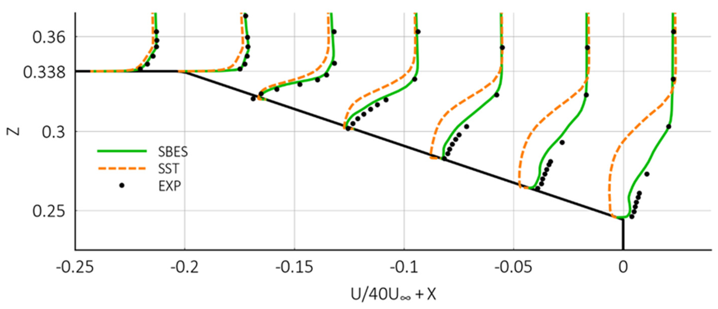
Figure 11 shows a comparison of RANS and SBES velocity profiles around the back of the car. The SBES formulation captures the experimental data with high accuracy and corrects the known deficiency of over-separation of RANS models (here SST) for this case.

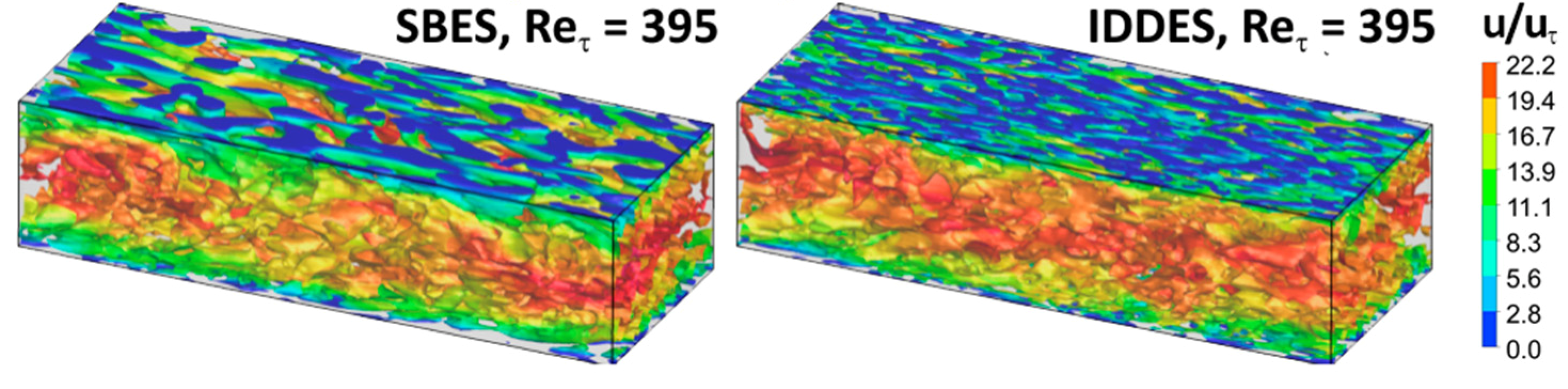
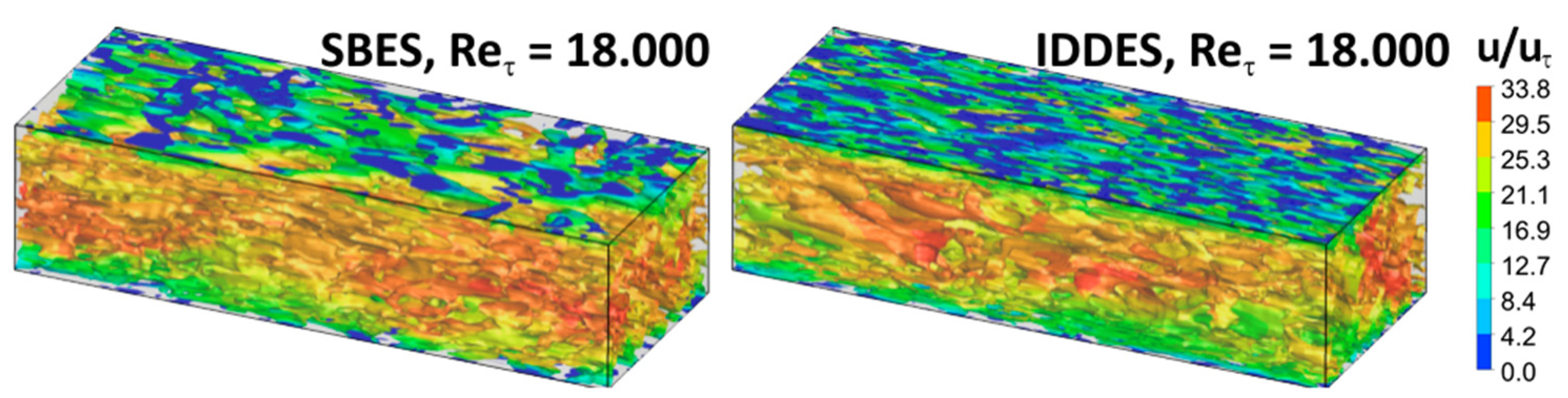
Another interesting characteristic of the SBES model is that it can operate in WMLES mode, once triggered into scale-resolving mode. This can be seen in Figure 12 for a channel flow. All grids are in the range of 500,000 cells, with y + ~1. The simulations were started from a LES solution to trigger the SBES model into SRS mode. Interestingly, SBES produces similar resolved structures as IDDES, which was specifically designed for this purpose. It needs to be stressed that IDDES does not provide the strong shielding capabilities of SBES in RANS mode, and therefore is only of limited use in industrial flows. 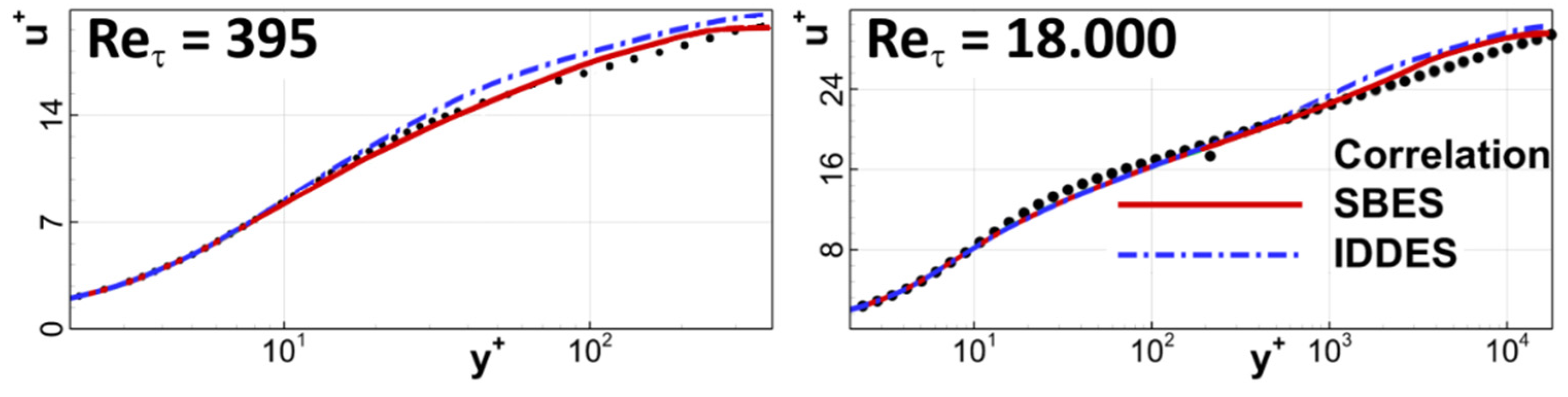Figure 13 shows the corresponding time-averaged velocity profiles in logarithmic scale. Both IDDES and SBES show a slight mismatch near the RANS–LES interface for the high-Re case, however capture the overall flow with good accuracy ($R{e}_{\tau }=u_{\tau }h/\nu$ with $u_{\tau }$- friction velocity, h = half height of the channel, $\nu$ = kinematic viscosity).

The option to run SBES inside the boundary layer in both RANS and WMLES models offers many interesting opportunities. It allows complex geometries to be run and triggers the WMLES mode only once the mesh is of sufficient resolution to support it. The triggering process can be initiated by a synthetic turbulence generator.

GEKO-Based SBES

When running global hybrid models in standard mode, the boundary layer is covered entirely by the RANS model. This saves large amounts of computational power but carries the uncertainties of RANS modeling into the hybrid simulation. The main issue is obviously the ability of the RANS model to accurately capture separation. Our research group recently developed a new RANS model, termed the Generalized k-ω (GEKO) model (Menter et al. [40,41]). It allows the re-calibration or fine-tuning of the model through user-exposed coefficients. The coefficients are designed in such a way that changing them (within defined limits) does not alter the basic model calibration for the flat plate. This allows non-turbulence experts to adjust the model to their applications. 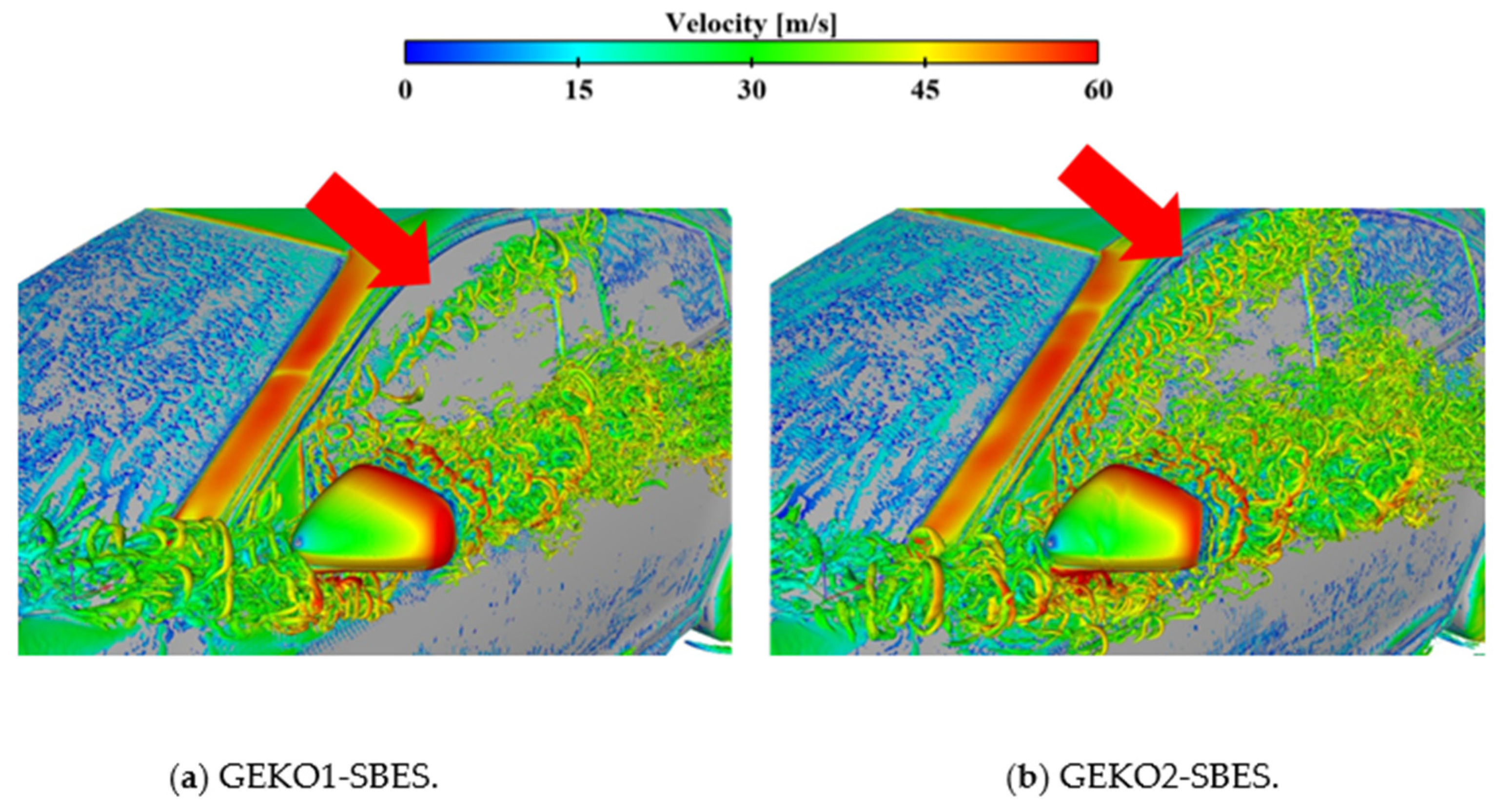An example of such an approach is the simulation of an automotive configuration with the goal of computing the noise from the side-mirror and the A-pillar of car onto the window, as reported by Zore and Caridi [42]. For the A-pillar noise, the correct separation prediction of the pillar vortex is essential. Figure 14 shows the region of interest. Two GEKO settings are used, one with the free coefficient GEKO1 with C_SEP = 1.0 and GEKO2 with C_SEP = 2.0. C_SEP is the main parameter in the GEKO model controlling separation onset. C_SEP = 1.0 corresponds to a k-ε model (with known late separation) and C_SEP = 2.0 is “aggressive” in predicting separation (even earlier separation prediction than SST). The difference between these two settings is clearly visible for the A-pillar vortex (red arrow), where the vortex is shifted downwards for the C_SEP = 1 configuration.

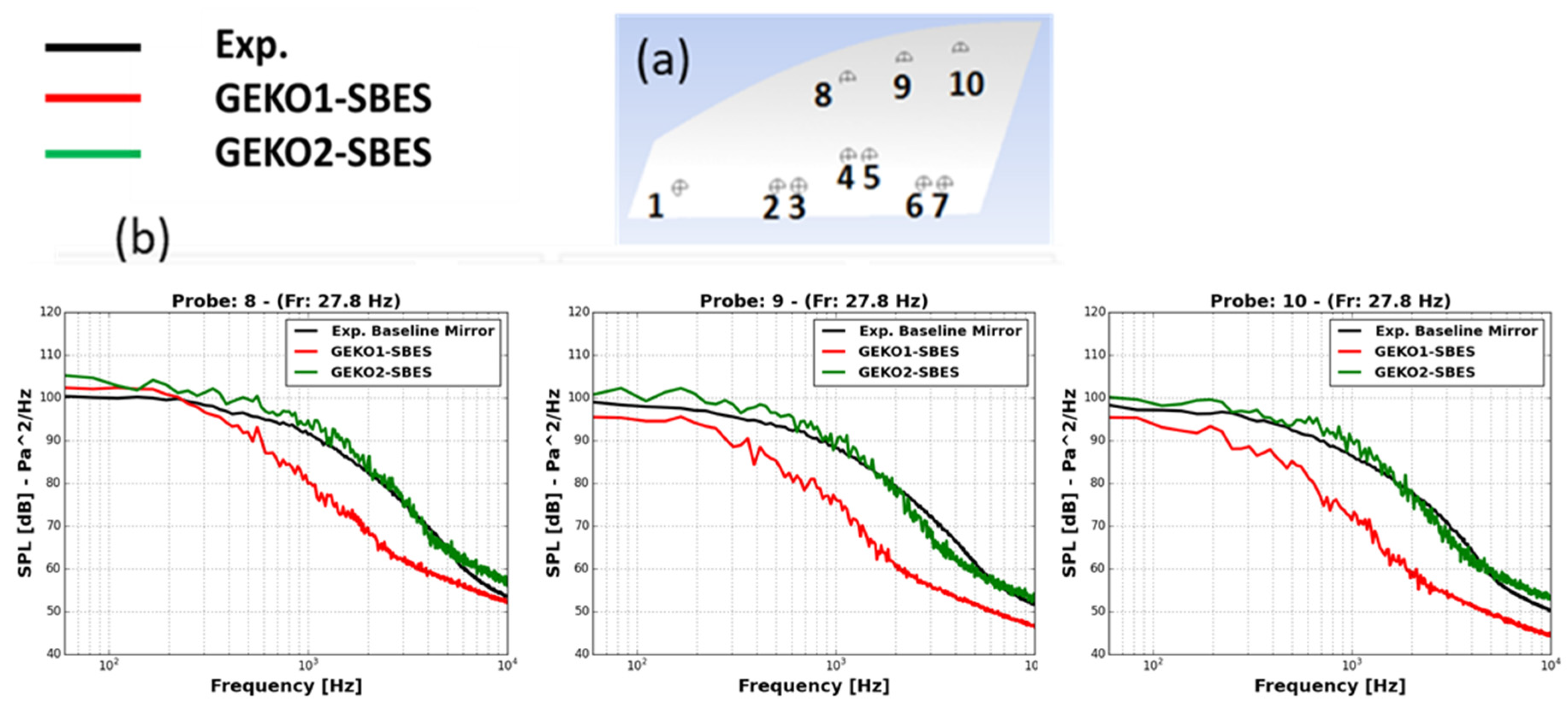
Figure 15 shows the sound pressure levels at the locations of the window affected by the A-pillar vortex. The positions in Figure 14a refer to the side-window locations—only positions 8, 9 and 10 are depicted, as they are the ones affected by the A-pillar vortex. The more aggressive setting using C_SEP = 2.0 (GEKO2) is in much better agreement with the data than C_SEP = 1.0 (GEKO1). This illustrates the advantage of combining a tunable RANS model with a hybrid RANS–LES method. This is important, as contrary to LES, the performance of the RANS part of the model cannot be improved by mesh refinement.

4. Embedded LES (ELES)

ELES is an approach whereby zones for RANS and LES are pre-defined—typically with the LES zone embedded into a larger RANS zone. In such a set-up, one typically employs a synthetic turbulence generator method, which converts RANS turbulence from upstream of the RANS–LES interface to LES content downstream of the interface.

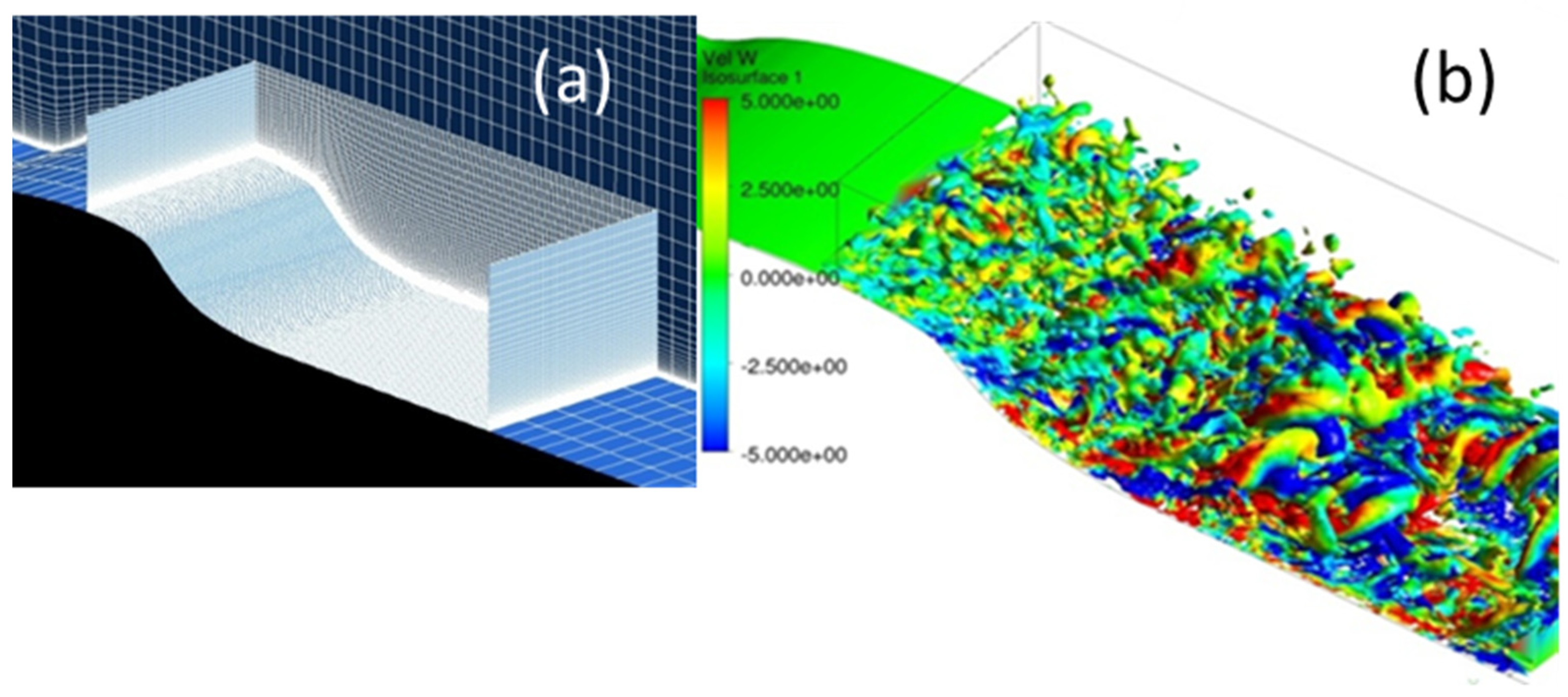
A challenging test case for ELES is the flow over a hump with a relatively large separation zone on the leeward side. Figure 16 shows the setup (Greenblatt et al. [43]), with an LES zone embedded into a wider RANS zone. The RANS region was computed with the SST model [44] and the LES zone with a WALE [45] and separately with a WMLES model [15]. At the RANS–LES interface, synthetic turbulence was generated using the method proposed by Shur et al. [15]. The LES grid consisted of 2 million hex cells. The momentum thickness Reynolds number of the boundary layer just upstream of the LES zone was high, with $R{e}_{\mathsf{\Theta }}=U_{\delta }\mathsf{\Theta }/\nu =7000$ ($U_{\delta }$ = boundary layer edge velocity, $\mathsf{\Theta }$ = momentum thickness, $\nu$ = kinematic viscosity).

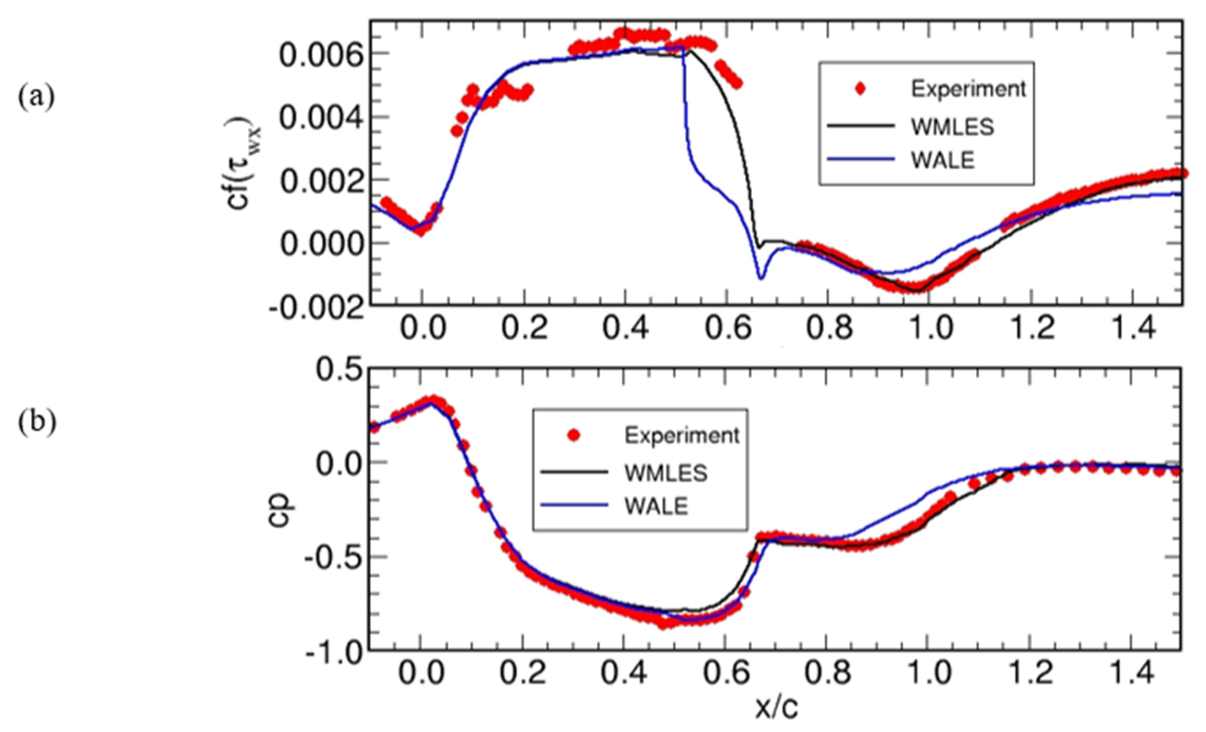
Figure 17 shows the skin friction and wall pressure coefficient distributions from the simulations. The use of the algebraic WMLES model [15] in the LES zone results in very close agreement with the data, even though the skin friction is known to be very sensitive to simulation details. Interestingly, in the simulations using the WALE model, the wall shear stress drops off immediately after the RANS–LES interface to unrealistically small values due to the lack of resolution. This is expected, as the Reynolds number is too high for a WRLES on the given grid. The use of a WMLES with the RANS layer close to the wall can remedy this shortcoming and provide good agreement with the experimental data.

One of the weak points of the current ELES models is that there is no ability to convert back LES results to RANS at the outflow of the LES zone. This is acceptable in some cases but not in all, and can create inconsistencies downstream of the LES zone. An alternative proposal for handling such situations is given by Xiao et al. [22].

5. Summary and Outlook

Substantial progress has been made in the last two decades in the development of reliable hybrid RANS–LES methods. For the current group, the SBES model offers an optimal platform for the different application scenarios for such approaches, as SBES can be run in classical DES-like mode, whereby the boundary layers are covered by RANS and free shear flows are covered by LES methods. In addition, SBES can operate in WMLES mode inside boundary layers when triggered by either synthetic turbulence or upstream obstacles, such as a backward-facing step. SBES is also computationally efficient, as it allows a delayed update of the two-equation RANS model portion, resulting in costs per iteration close to those of a pure LES model. Last but not least, the approach is generic and allows the combination of existing RANS and LES models, which is especially attractive for industrial codes with many models, both on the RANS and the LES sides.

The question remains of what the will future bring. Clearly, with the combination of exiting RANS and LES methods in the generic SBES formulation, improvements for both RANS and LES methods can be directly integrated into the hybrid model. In other words, any improvement on either modeling side will automatically lead to improvements in the hybrid RANS–LES formulation.

Both RANS and LES formulations will benefit from Machine Learning (ML), as can be anticipated from RANS studies (e.g., Duraisamy et al. [46]) and LES studies (e.g., Beck et al. [47]). The potential might be higher on the LES side, as the RANS part mainly influences the boundary layer and can be already controlled quite flexibly by the free parameters of the GEKO model. ML for LES could potentially lead to large reductions in computation effort in the LES zone, thereby significantly reducing the turn-around time. Considering that most ML techniques for LES are carried out on Cartesian meshes, hybrid RANS–LES methods might be well-positioned to benefit from ML, as the LES part away from walls can often be covered by Cartesian-dominated grids (octree).

The application of WFLES and WMLES inside boundary layers is a much more difficult problem. The resolution requirements are still too high for realistic Reynolds numbers, and flexible methods will be required that allow the upstream thin boundary layers to be handled in RANS mode (including the laminar–turbulent transition) and to automatically trigger the simulation into LES mode once the mesh is fine enough to resolve the boundary layer turbulence.