Article

3D Texture Feature Extraction and Classification Using GLCM and LBP-Based Descriptors

Communications Department, Technical University of Cluj-Napoca, 400114 Cluj-Napoca, Romania
*
Author to whom correspondence should be addressed.
Appl. Sci. 2021, 11(5), 2332; https://doi.org/10.3390/app11052332
Submission received: 10 February 2021 / Revised: 25 February 2021 / Accepted: 2 March 2021 / Published: 5 March 2021
(This article belongs to the Section Computing and Artificial Intelligence)

Abstract

:
Lately, 3D imaging techniques have achieved a lot of progress due to recent developments in 3D sensor technologies. This leads to a great interest regarding 3D image feature extraction and classification techniques. As pointed out in literature, one of the most important and discriminative features in images is the textural content. Within this context, we propose a texture feature extraction technique for volumetric images with improved discrimination power. The method could be used in textured volumetric data classification tasks. To achieve this, we fuse two complementary pieces of information, feature vectors derived from Local Binary Patterns (LBP) and the Gray-Level Co-occurrence Matrix-based methods. They provide information regarding the image pattern and the contrast, homogeneity and local anisotropy in the volumetric data, respectively. The performance of the proposed technique was evaluated on a public dataset consisting of volumetric textured images affected by several transformations. The classifiers used are the Support Vector Machine, k-Nearest Neighbours and Random Forest. Our method outperforms other handcrafted 3D or 2D texture feature extraction methods and typical deep-learning networks. The proposed technique improves the discrimination power and achieves promising results even if the number of images per class is relatively small.

1. Introduction

The image classification domain has received a lot of interest from researchers due to its significant contribution and successful implementation in different applications from the biomedical domain, remote sensing, industry and many more. The task of image classification involves the prediction of a class from a set of predefined categories for a given input image by taking into consideration its visual content [1]. Even if the components of an image classification system depend on the specific application in which the system is used, two processes are always needed in any supervised machine-learning image classification task: training and testing. The training step uses a training set of images for which the categories to which they belong are known. These images are analysed by using a feature extraction technique, which is used to provide the most important and discriminative features in an image (stored as a feature vector). In the testing step, as input for the classification system, a new image is used, and the goal of this step is to predict the membership class of that image [2]. The same feature extraction method is used to determine the feature vector for the new image. At this point, a classification operation is used to compare this feature vector with the ones obtained in the training phase and to assign the new image to the nearest class based on a specific criterion.
The feature extraction step is the most important in such a task since the machine-learning algorithm operates on the extracted features [3]. The image analysis process is used to obtain a reduced representation of the images by keeping only the most important information. If the features are not sufficiently relevant and discriminative, even the most powerful machine-learning algorithm cannot achieve a good performance. The discrimination power is gained by descriptors that provide low intra-class variability and high variability between different classes [4]. The image classification task is a challenging one because images are exposed to different illumination conditions, can be affected by noise and can suffer different transformations. That is why the extracted features should provide invariance and robustness to these conditions in order to achieve a good classification performance.
One of the most important characteristics of images is the texture. This is true especially for medical images where the textural features and the statistical indicators (such as kurtosis, entropy) are the most relevant for the detection of several diseases, such as breast cancer [5]. The textural description of images was implied in many feature extraction techniques proposed in literature. Most of them were mainly focused on 2D textured images. Volumetric image analysis and classification is of interest nowadays due to the progress gained concerning 3D sensor technologies and imaging techniques [6]. In the medical domain, 3D images are widely used in computer-aided diagnostic systems that are based on images acquired, for example, by magnetic resonance imaging (MRI), computed tomography (CT) and ultrasound techniques. Such volumetric images are represented as data cubes, so feature extraction methods should be adapted to deal with this type of data. Since texture is a very important feature of medical images, powerful and discriminative texture feature extraction methods are needed to achieve a reliable classification of such images, taking into consideration that for volumetric images, the computation complexity is a challenging problem.
Due to the progress gained in the 3D imaging domain, the interest regarding volumetric texture feature analysis methods increased. Even if 2D feature extraction methods can still be applied on slices of 3D images, this strategy would disregard the relations between slices. The disadvantage of such an approach is the information loss in the propagation of texture along the neighbouring slices. The 3D feature extraction field is significantly less developed than the 2D one. Most of the 3D feature analysis methods are extensions of efficient and popular 2D descriptors. Such descriptors include the Local Binary Patterns operator [7], which was extended to 3D in [8]. If, in the 2D formulation, each pixel is compared to its neighbours located on a circular neighbourhood, in the 3D extension of LBP addressed in [3], the authors define neighbours on a sphere. Since the dimensionality is a problem in the 3D space, a uniformity criterion is used to reduce the number of possible patterns. In the 2D case, this criterion involves the usage of patterns with at most two bitwise transitions in the pattern. We refer to the original publication, [7], for further details. For volumetric images, the authors propose relaxing the criterion to allow up to three transitions. A 2D LBP-derived operator, the Extended Local Binary Patterns (ELBP), was adapted to deal with volumetric images in [9]. A rotation invariant 3D extension based on the LBP descriptor was introduced in [10] where the authors considered using precomputed 2-patterns.
Another efficient texture descriptor besides LBP is the Gray-Level Co-occurrence Matrix (GLCM) which is used as a tool in order to derive second-order statistics from 2D textured images. An extension of GLCM to volumetric images is proposed in [11]. This method is similar to its 2D variant, but the displacement vector is defined by using three coordinates and a higher number of orientations. Another extension to 3D involves the volumetric run-length matrix from which several texture features are used to describe 3D data [12].
Application of volumetric texture analysis methods in the medical domain has become more and more prevalent in recent years. The magnetic resonance imaging (MRI) technique is very important for the medical domain, being a tool used in diagnostic systems. Thus, there is a high interest to develop powerful feature extraction and classification algorithms adapted to this type of images in order to make the distinction between healthy and non-healthy tissue. In [13], the authors propose a feature extraction technique for the classification of magnetic resonance images involving malignant or benign breast lesions. For segmentation of lesions, a fuzzy c-means clustering-based method is used. The features are extracted from a nondirectional GLCM which is obtained by summing all directional GLCMs for all 13 independent directions. In [14], magnetic resonance images of the brain are classified using as feature descriptor multi-sort co-occurrence matrices. This implies considering several axes and combining different features in a multidimensional matrix. In [15], MRI images of knees are analysed by considering a sub-band filtering method. For reducing the size of the feature vector, a feature selection algorithm based on the Bhattacharyya distance measure is proposed. Lately, for the classification of MRI images, different deep-learning-based methods have been proposed in literature, such as [16], where the authors compare three different types of Convolutional Neural Networks (CNN) for the classification of brain MRI images. Another example of brain tumour classification performed on MRI images is [17], where the authors propose a new CNN architecture that can be used to help medical experts to carry out a diagnostic.
Other methods used for volumetric image texture feature extraction include using Locally Oriented Wavelet Transforms as in [18]. The three-dimensional Gaussian Markov Random Fields are employed in [19] for the detection of COPD (chronic obstructive pulmonary disease) by considering a dataset containing images of lungs acquired by the computer tomography imaging technique. Another paper that uses Gaussian Markov Random Fields for the analysis of volumetric textures performs the discrimination of soft tissue from abdomen CT images [20].
The paper is structured as follows. Section 2 reviews the original LBP operator along with an improved variant and the 2D and 3D versions of the GLCM feature extraction technique. Section 3 describes the proposed method, a 3D texture feature extraction technique for the analysis of volumetric images. Section 4 describes the experimental setup, Section 5 presents the obtained results, while the conclusions are given in Section 6.
The proposed approach fuses two complementary feature vectors: a feature vector derived from the 3D version of the Block Matching and 3D Filtering Extended Local Binary Patterns (BM3DELBP_3D) operator and a feature vector generated by the Improved 3D Gray-Level Co-occurrence Matrix (IGLCM_3D). BM3DELBP_3D provides features that are robust to Gaussian noise and have good invariance properties. The extracted features are based on the sign of the difference between pixels, but the magnitude of the difference is not taken into consideration. This type of information is generated by the complementary feature vector given by the Improved 3D Gray-Level Co-occurrence Matrix. This method computes co-occurrence matrices based both on image intensity information and on the gradient image.

2. Background

2.1. Local Binary Patterns (LBP)

The Local Binary Patterns (LBP) operator is a texture descriptor that is widely used in literature in many computer vision applications due to its efficiency in describing local texture structures, simplicity, speed of computation and robustness to illumination variations [7]. The LBP operator provides a local representation of textured images which is obtained by computing differences between neighbouring pixels. By considering a neighbourhood around each pixel, an LBP code is computed for each image spatial location. The feature vector is obtained by computing the histogram of all LBP codes. The improved LBP variant proposed in [7] (based on the original formulation [21]) considers circular neighbourhoods of variable sizes which allows the generation of texture features at different scales. By adopting a multi-resolution approach as proposed in the same paper, a degree of invariance to the change of the observation scale can also be attained. The multi-resolution strategy implies the concatenation of feature vectors obtained at different scales. The authors also propose a uniformity criterion in order to improve the rotation invariance of the extracted features. The uniform patterns are the ones with at most two bitwise transitions in the pattern. As pointed out in [7], if there is a large number of spatial transitions in the pattern, it is more likely that the pattern will change to a different one during rotation. The uniformity criterion improves the rotation invariance, but also reduces the size of the feature vector. Moreover, a noisy pattern creates fluctuations below or above the value of the central pixel due to the random character of the noise which results in many transitions in the pattern. By considering the uniformity criterion, the noisy patterns are considered as non-uniform and are discarded instead of being interpreted as a strong contrast between the central pixel and its neighbours. The number of transitions is expressed by a uniformity function, U . The uniform rotation invariant LBP (riu2) is computed using:
  LBP R , P riu 2 ( x c )   = n = 0 P 1 s ( x c   x R , P , n ) ,   if   U ( LBP R , P )     2 P + 1 ,   otherwise
where x c is the central pixel, s(x) is the sign function given in (2),   x R , P , n is the n th neighbour pixel from a neighbourhood having P neighbours and a radius R and U is the uniformity function;
s x = 0 ,   if   x < 0 1 ,   if   x 0
In a neighbourhood with P neighbours, there are exactly P + 1 uniform patterns. Each uniform pattern is labelled separately depending on the number of bits of 1 in the pattern, but all non-uniform patterns are labelled together under the mixed label P + 1. The histogram corresponding to the obtained LBP codes has a number of P + 2 bins. The non-uniform patterns can be discarded and thus, the final feature vector is of size P + 1 [7].

2.2. Block Matching and 3D Filtering Extended Local Binary Patterns (BM3DELBP)

Even if the LBP operator is efficient in many texture classification problems, it has a great disadvantage: the noise sensitivity. In order to handle this issue and to increase the discrimination power of the LBP, we proposed in a previous work [22], the Block Matching and 3D Filtering Extended Local Binary Patterns (BM3DELBP) operator which was inspired by the Median Robust Extended Local Binary Patterns formalism [23]. Instead of considering raw pixel values like LBP, BM3DELBP introduces a filtering step in the feature extraction operation and considers responses to a state-of-the-art filter, the Block Matching and 3D Filtering (BM3D) [24]. Thus, the vulnerability to noise is addressed by using this denoising technique, which is able to attenuate high levels of Gaussian noise without altering the texture structures for particular choices of the set of parameters. This is done by performing the denoising in the transform domain. In the first step, a grouping by block-matching is performed: 2D blocks that are similar to a reference block are stacked together in a 3D group. By considering a 3D transform, the signal is represented sparsely in the transform domain due to the similarity between the blocks that compose a group. In the 3D transform domain, a second step is performed: collaborative filtering. In this phase, the noise is eliminated by shrinking the transform coefficients, the textural features being still preserved. We refer to the original publication for more details regarding BM3D [24]. Despite recent developments addressing the use of deep-learning techniques in the image filtering domain, the BM3D collaborative approach remains one of the most performant [25].
The feature space of this operator is built by considering two types of features as in the Extended Local Binary Patterns [26]: pixel intensities and differences between pixel intensities. The first category includes two components: The central pixel intensity operator labelled BM 3 DELBP _ CI and the neighbours’ intensities component denoted by BM 3 DELBP _ NI R ,   P riu 2 :
BM 3 DELBP _ CI ( x c )   =   s ( x c C I )
where C I is the mean value of the entire input image, s(x) is the sign function given in (2) and x c is the central pixel;
BM 3 DELBP _ NI R ,   P riu 2 ( x c )   =   n = 0 P 1 s ( x R , P , n u R ) ,   if   U ( BM 3 DELBP _ NI )     2 P + 1 ,   otherwise
where u R is the mean value of the neighbouring pixels, being given in (5),   x R , P , n is the n th neighbour pixel from a neighbourhood having P neighbours and a radius R, U is the uniformity function and the superscript riu2 indicates the use of uniform rotation invariant patterns that have U     2 ;
u R   =   1 P × n = 0 P 1 x R , P , n
The second category contains one component based on differences between pixel intensities, the radial difference operator which is denoted by BM 3 DELBP _ RD R ,   P riu 2 :
BM 3 DELBP _ RD R ,   P riu 2 ( x c )   =   n = 0 P 1 s ( x R , P , n x R 1 , P , n ) ,   if   U ( BM 3 DELBP _ RD )     2 P + 1 ,   otherwise
where R and R − 1 are the radii of two circles on which the considered pixels are located.
Figure 1 shows the diagram which describes the BM3DELBP feature extraction process. A textured image is used as input for the feature extraction system. Then, the input image is filtered using BM3D for reducing the noise. The multi-resolution strategy is used for providing a degree of invariance to the observation scale: the features extracted from each scale of interest are concatenated. The considered scales are the ones having the radii 2, 4, 6 and 8. They were chosen by trial and error such that the computed operator is able to discriminate features at smaller scales (R = 2 and R = 4) but also at larger scales (R = 6 and R = 8). For each scale, the three operators given in (3), (4) and (6) are computed and the resulting codes are fused together into a joint histogram. The histogram of the central pixel intensity operator has 2 bins and the histograms corresponding to the other two operators have P + 2 bins, but only P + 1 bins correspond to uniform patterns. Thus, the joint histogram is of size ( P + 1 )   ×   ( P + 1 )   ×   2 . The final histogram, which is used as texture descriptor of the input image, is obtained by concatenating all joint histograms for all considered scales.

2.3. 2D Gray-Level Co-Occurrence Matrix (2D GLCM)

The Gray-Level Co-Occurrence Matrix (GLCM) is a classical texture feature extraction technique proposed in 1973 by Haralick [27]. To make the article self-contained and for a better understanding, we briefly review below how the 2D GLCM is built.
GLCM is a statistical method that takes into account the spatial relationship between pixels. This matrix is not the feature vector itself, is rather a tool for obtaining second-order statistics.
The GLCM expresses the frequency of appearance of pairs of pixels which are situated at a certain distance and orientation to each other and which have certain grey-level intensities. The two elements that characterize the spatial relationship between pixels define the displacement vector:
d   =   ( d x , d y )
Generally, the orientation for 2D GLCM is considered for four independent directions which are given in Figure 2. Table 1 shows the corresponding displacement vectors.
The GLCM is a square matrix, having N q rows and N q columns ( N q is the number of different pixel values in the input image). The input image can be scaled in order to reduce the number of grey-levels. Generally, the GLCM is built on images that have 8, 16, 32 or 64 quantization levels. This is done for providing statistical confidence: the matrix must contain a reasonably non-sparse representation. Additionally, a smaller number of quantization levels implies reducing the computation time.
The coefficients of the GLCM are expressed in terms of probabilities rather than in number of appearances by performing normalization: the terms are divided by the total number of possible combinations (the sum of the matrix values). The normalized GLCM is given in (8):
GLCM _ 2 D n i , j   =   GLCM _ 2 D ( i , j ) i = 1   N q j = 1   N q GLCM _ 2 D ( i , j )
where GLCM _ 2 D n is the normalized version of GLCM _ 2 D which is given in (9):
GLCM _ 2 D d x , d y i , j   =   x = 1 m y = 1 n 1 ,   if   I x , y   =   i   and   I x + d x , y + d y   =   j 0 ,   otherwise
where I is the input image of size m × n .
The feature vector is obtained by computing the Haralick indicators [27] from the obtained normalized GLCM. We refer to [27] for a complete description of these statistical indicators.

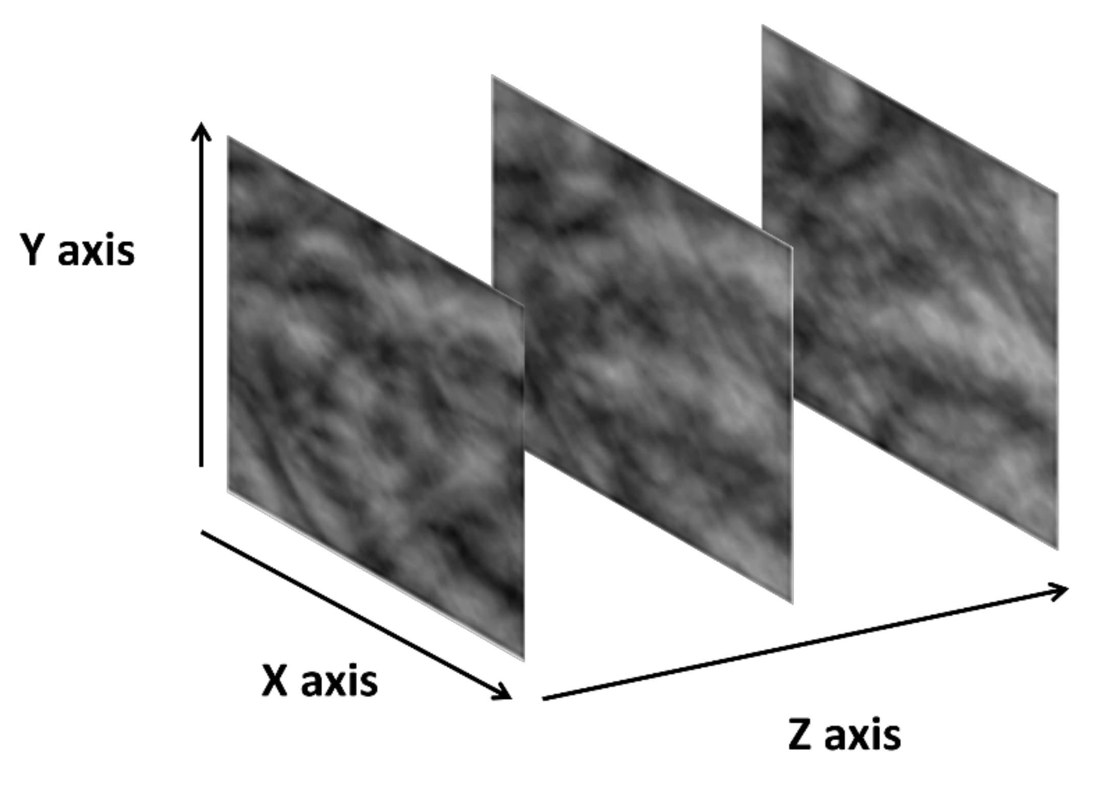
2.4. 3D Gray-Level Co-Occurrence Matrix (3D GLCM)

The 2D GLCM was extended to 3D [11] in order to be able to capture information between different slices of a volumetric image. The displacement vector has three components as defined in (10):
d   =   ( d x , d y , d z )
In this case, the orientation is defined for 13 independent directions. Table 2 shows the 13 corresponding displacement vectors.
Let I be an input volumetric image of size m × n × p voxels. The 3D GLCM of I is given in (11) and its normalized version in (12):
GLCM _ 3 D d x , d y , d z i , j   =   x = 1 n y = 1 m z = 1 p 1 ,   if   I x , y , z   =   i   and   I x + d x , y + d y , z + d z   =   j 0 ,   otherwise
GLCM _ 3 D n i , j   =   GLCM _ 3 D ( i , j ) i = 1   N q j = 1   N q GLCM _ 3 D ( i , j )
where GLCM _ 3 D n is the normalized version of GLCM _ 3 D .
We also had prior contributions in this thematic area by proposing a 3D version of the BM3DLEBP operator and a more discriminative 3D GLCM based on which we built the proposed method. We describe the two proposed methods and the feature vectors’ fusion in the subsequent section.

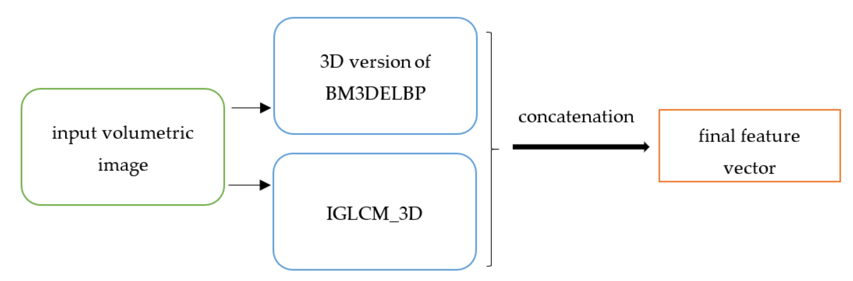
3. The Proposed Method

The proposed method covered in the article extends our prior contributions validated in the two conference papers [28] and [29] by fusing the two results and provides a complex means of feature description in 3D. In [28], we proposed the 3D version of BM3DELBP (BM3DELBP_3D) whose feature space is constructed based on the signs of differences between neighbouring pixels without any information regarding the amount of difference such as the contrast or degree of homogeneity in the analysed image. This knowledge is captured by the Improved 3D Gray-Level Co-Occurrence Matrix (IGLCM_3D) introduced by us in [29]. Following, the proposed approach described by the current paper aims at the combination of the two types of texture features in order to increase the discrimination power. Figure 3 summarizes the feature extraction process of the proposed technique.

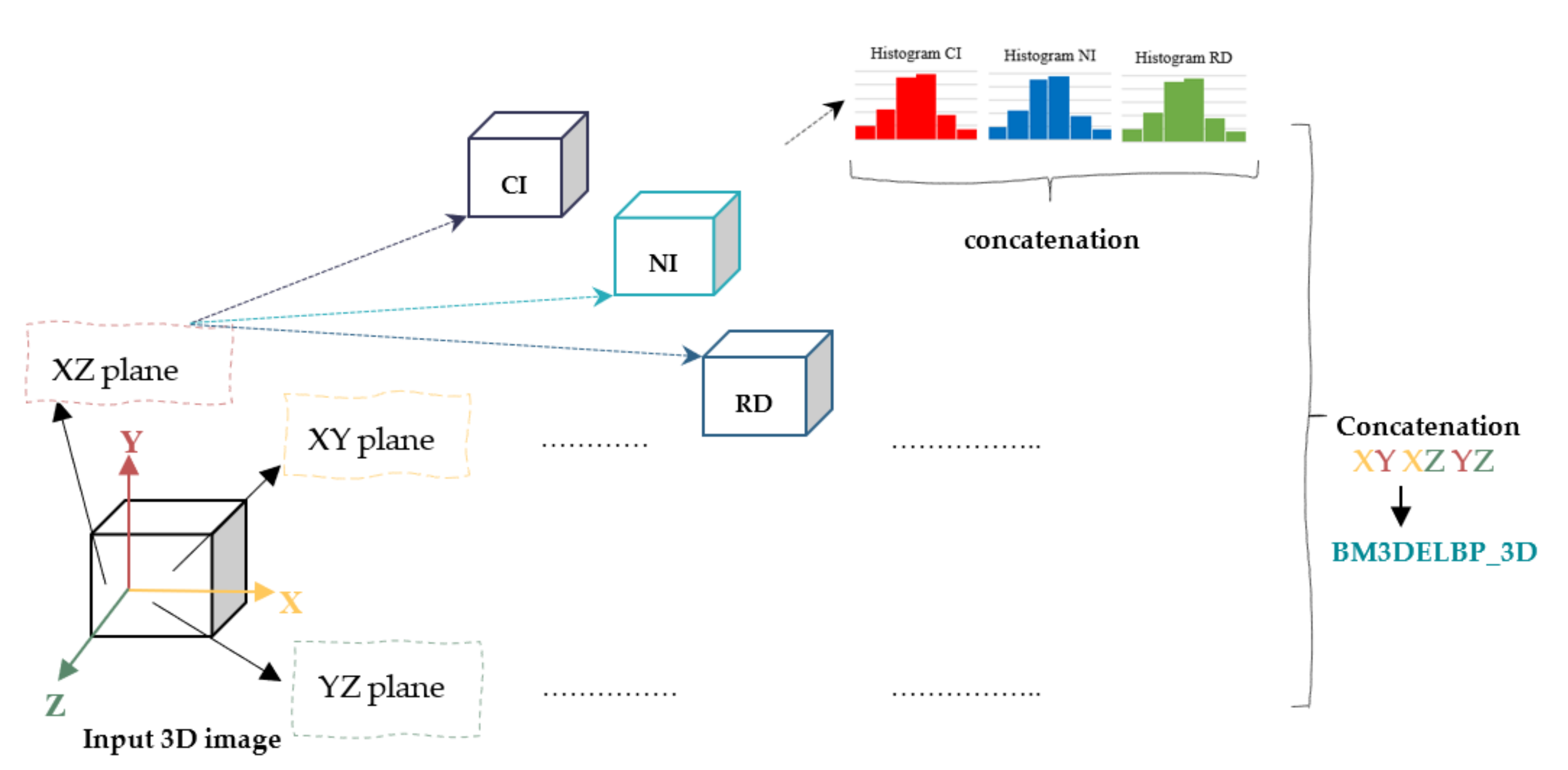
3.1. The Extension of BM3DELBP to 3D (BM3DELBP_3D)

We proposed in [28] the extension of the BM3DELBP operator to volumetric texture feature extraction. Figure 4 illustrates the functional block scheme describing the computation of this operator by considering only one observation scale.
For each 3D input image, the BM3DELBP codes are extracted separately from each of the three orthogonal planes XY, XZ and YZ. As the input image is a cube, for each plane, there are several image slices. The BM3DELBP operator is thus applied separately on each slice of each plane. For each slice, the BM3D denoising technique is applied and then, by considering the responses to the applied filter, the three components of the BM3DELBP operator are computed: BM3DELBP_CI, BM3DELBP_NI and BM3DELBP_RD. The feature vector corresponding to one orthogonal plane results from the concatenation of the histograms obtained for each volumetric component. A multiresolution strategy is used to attain a degree of invariance to the change of the observation scale based on the same strategy described in Section 2.2. Two scales were considered given by their radius: R = 2 and R = 4, respectively. In [22], four scales were used for 2D image classification. Since we deal with volumetric images and the computation complexity is challenging, we proposed reducing the number of scales to two in order to minimize the feature vector size and to avoid the classic curse of dimensionality problem. Figure 5 presents the considered multiresolution strategy for the 3D case.
The operations involved are the ones from Figure 4 and they are considered for both scales of interest, the resulting feature vector being obtained by concatenation.

3.2. The Improved 3D Gray-Level Co-Occurrence Matrix (IGLCM_3D)

3.2.1. Definition and Method Overview

We proposed in the preliminary work [29] an improved version of the 3D GLCM, the IGLCM_3D. The functional diagram is given in Figure 6.
As shown in Figure 6, the feature extraction process is based on the computation of 4 types of co-occurrence matrices. The first one is the 3D standard GLCM defined in (12), which is computed directly from the input image intensities. The other three types of 3D co-occurrence matrices are based on the gradient image information. This can depict the distribution of strong or weak edges and the degree of uniformity of the input image. The matrix based on the gradient magnitude information is labelled Gradient Magnitude Co-Occurrence Matrix (GMCM) and is given in (13) for an input image I of size m × n × p .
GMCM d x , d y , d z i , j   =   x = 1 m y = 1 n z = 1 p 1 ,   if   M x , y , z   =   i   and   M x + d x , y + d y , z + d z   =   j 0 ,   otherwise
where M   =   G X 2 + G Y 2 + G Z 2 is the gradient magnitude and G X , G Y and G Z are the components of the gradient vector in the three directions.
The other two 3D co-occurrence matrices are based on the gradient orientation, which offers additional information about the local anisotropy for the considered textured images. The two matrices are labelled Azimuth Angle Co-Occurrence Matrix (AACM) and Elevation Angle Co-Occurrence Matrix (EACM), given in (14) and (15), respectively:
AACM d x , d y , d z i , j   = x = 1 m y = 1 n z = 1 p 1 ,   if   θ x , y , z   =   i   and   θ x + d x , y + d y , z + d z   =   j 0 ,   otherwise
where θ   =   tan 1 ( G Y G X ) is the azimuth angle.
EACM d x , d y , d z i , j   =   x = 1 m y = 1 n z = 1 p 1 ,   if   Φ x , y , z   =   i   and   Φ x + d x , y + d y , z + d z   =   j 0 ,   otherwise
where Φ   =   tan 1 ( G Z G X 2 + G Y 2 ) is the elevation angle.

3.2.2. Computation of the Haralick Feature Vector

The 3D GLCM is computed from the quantized image by considering the image intensities information of the input volumetric cube. The number of quantization levels is N q   =   32 , chosen as a trade-off between time efficiency and loss of data. The considered directions are all 13 independent directions provided in Table 2 and the considered distances are: 1 voxel and 2 voxels, respectively. The GLCM matrix is generated for all considered orientations and distances, resulting 26 matrices (13 directions × 2 distances). All matrices are normalized. The computed GLCM does not constitute the feature vector, it is just a tool used to compute different statistical indicators. For the GLCM matrix, 14 Haralick indicators [27] are determined: energy, entropy, correlation, contrast, homogeneity, variance, sum average, sum entropy, sum variance, difference entropy, difference variance, information measures of correlation 1 and 2 and the maximal correlation coefficient. They are computed for each of the 26 obtained matrices. The Haralick feature vector (GLCM feature vector) is obtained by considering the block scheme from Figure 7.
For each distance, there are 14 Haralick indicators calculated for each of the 13 directions. For each Haralick indicator, the average and standard deviation are computed for all directions in order to gain a degree of invariance to rotation. By concatenating the features obtained for the two considered distances, a degree of invariance to the observation scale is also obtained. The final Haralick feature vector contains 56 characteristics as detailed in the Appendix A.

3.2.3. Computation of the Three Gradient-Based Matrices and the Corresponding Feature Vectors

Figure 8 illustrates the block diagram describing the computation of the gradient-based matrices.
The following four steps are considered: noise reduction, computation of the gradient image, computation of GMCM, AACM and EACM matrices and of the feature vectors.
The three co-occurrence matrices are based on the gradient image. In order to prevent the detection of false edges caused by noise, we employ a 3D Gaussian smoothing filter. The considered parameters for this filter were chosen as a trade-off between noise elimination and attenuation of edges: the size of the kernel is of 5 × 5 × 5, the mean of the 3D Gaussian function is 0 and the standard deviation is σ   =   2 . For preventing illumination changes, a normalization is performed at the end of this step.
For computing the gradient image, the 3D Sobel operator is used since it offers noise robustness and computational efficiency. The considered 3D Sobel masks are the ones provided by Matlab [30].
After the computation of the gradient image, three parameters are obtained: the gradient magnitude given in (13), gradient azimuth angle given in (14) and gradient elevation angle given in (15). They are quantized using 32 levels and used for constructing the GMCM, AACM and EACM matrices. The three matrices are computed for all 13 independent directions and two distances (1 voxel and 2 voxels) and are normalized after computation.
In the last step, three feature vectors are computed: the GMCM feature vector (gradient magnitude-based feature vector), the AACM feature vector (azimuth-based feature vector) and the EACM feature vector (elevation-based feature vector).
The gradient magnitude-based feature vector is extracted from the GMCM matrix. As gradient-based indicators, we proposed in [29] the following measures:
  • Quantity of strong edges (Q):
Q   = i = 1 Nq j = 1 Nq ( i j ) 2 × GMCM n ( i , j )
where GMCM n is the normalized version of GMCM.
A high value for Q indicates that there are many strong edges. This indicator favours substantial gradient changes for neighbouring voxels in the considered image.
  • Slightly textured image indicator (STI):
STI = i = 1 Nq j = 1 Nq 1 1 + ( i j ) 2 × GMCM n ( i , j )
This indicator favours voxel pairs situated near the principal diagonal and implies that the encountered edges are weak, so the considered input image is slightly textured.
  • Uniformity (U):
U = i = 1 Nq j = 1 Nq ( GMCM n ( i , j ) ) 2
A large value for U means that there are high values in the GMCM matrix. Since this matrix is normalized and its terms are expressed as probabilities, this implies that there are only a few high values. This leads to the conclusion that there are few edges and the image presents textural uniformity.
  • Strong edges indicator (S):
S = i = 1 Nq j = 1 Nq i 2 ×   GMCM n ( i , j )
S favours large gradients, a high value indicating that there are many strong edges in the analysed textured image.
These indicators are computed for each GMCM matrix. The gradient magnitude-based feature vector is obtained by considering the same strategy used for the Haralick features as described in Figure 7. The final gradient magnitude-based feature vector contains 16 characteristics as detailed in appendix A.
The azimuth-based feature vector is computed from the AACM matrix by considering the entropy indicator:
Entropy _ 1   =   i = 1 Nq j = 1 Nq AACM n i , j × log AACM n i , j ,   for   AACM n i , j     0
The elevation-based feature vector is computed from the EACM matrix. The same indicator is used, the entropy:
Entropy _ 2   =   i = 1 Nq j = 1 Nq AACM n i , j × log EACM n i , j ,   for   EACM n ( i , j )     0
A high value for the entropy indicator is obtained for heterogeneous input textures and a low value for coherent textured images since the entropy describes the degree of randomness. In this context, the entropy is used to depict differences regarding the local anisotropy.
For building the two orientation-based feature vectors, this entropy indicator is computed for all AACM and EACM matrices and the same fusion strategy as for GLCM is used. The final azimuth-based feature vector contains four characteristics and the same is valid for the elevation-based feature vector.

3.2.4. Final Feature Vector Computation

Figure 9 describes the computation of the final feature vector of the IGLCM_3D. The Haralick feature vector, the gradient magnitude-based feature vector, the azimuth-based feature vector and the elevation-based feature vector are fused together by concatenation in order to form the final feature vector.

3.3. Fusion of the BM3DELBP_3D and IGLCM_3D Complementary Features

From (3), (4) and (6), we can see that the three components that define the feature space of the BM3DELBP_3D are based on the sign of the difference between pixels: between the central pixel and the mean of an entire slice, between the neighbouring pixels and their mean value and between the neighbouring pixels located on two circles with different radii. This means that only the sign of the difference is taken into account and no information regarding the amount of difference is considered. The BM3DELBP_3D operator does not provide any data related to the contrast of an image, to the degree of homogeneity, number of strong or weak edges and their quantity. This information is discarded completely. However, this type of information is actually generated by the IGLCM_3D matrix. Therefore, the supplementary knowledge gained by fusing the feature vectors of the two methods can be helpful in increasing the discrimination power.

3.4. Invariance Properties of the Proposed Method

The feature vector generated by our approach provides a degree of invariance to the change of the observation scale, to rotation and illumination conditions. Improved properties of scale invariance are obtained by considering four different circular neighbourhoods in the BM3DELBP_3D case and two distances for IGLCM_3D. The invariance to rotation is achieved by using the uniform rotation invariant coding strategy for BM3DELBP_3D. The disadvantage of IGLCM_3D is the fact that it is not inherently invariant to rotation. However, a degree of invariance to this transformation can be obtained by computing the mean and standard deviation across several directions. The illumination invariance is provided by BM3DELBP_3D since this is a key property of the original LBP. However, in the IGLCM_3D case, only the azimuth and elevation-based features are invariant to linear transformations of the illumination, as explained in detail in [29].

4. Experimental Setup
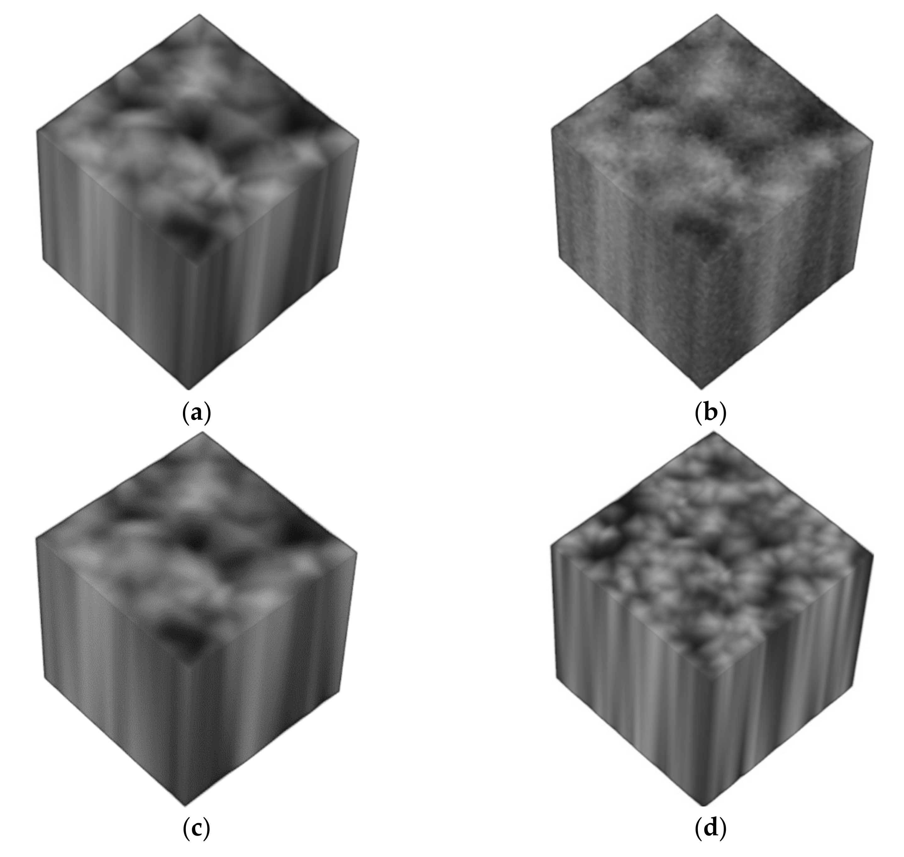
4.1. Dataset

In order to evaluate the proposed feature extraction technique, we used the RFAI dataset [31] which is publicly available. It is composed of volumetric synthetic textures of size 64 × 64 × 64 voxels. The authors in [31] considered several techniques for obtaining the 3D images: an interpolation strategy, a method based on the Fourier Transform, a random distribution of geometric shapes and a combination of all these methods. The first experiment was carried out by using the images built using the interpolation approach for which we selected 9 texture classes which are detailed in Table 3.
As in [32], we opt to use the images constructed by interpolation and the nine texture categories. As shown in the original publication, those classes are more similar to biological tissue. We considered 40 texture samples per class: 10 regular images that are not affected by any transformation, 10 smoothed samples upon which the Gaussian blur was applied, 10 noisy textures altered by Gaussian noise and 10 textures affected by a subsampling distortion. Figure 10 illustrates a regular sample for each of the nine categories.
Figure 11 presents some texture samples from category Blocks in order to exem-plify the applied transformations.
For better observing the fact that the images constructed by interpolation are true 3D volumes, we show in Figure 12 a regular image sample from class SinusSynthesis. We can see that the 2D pattern is not translated along the depth axis since the slices of the 3D images are not identical.
In the second experiment, we considered using all images from the RFAI database [31]: images built by interpolation, by using the Fourier Transform, by considering a random distribution of geometric shapes and a combination of all these methods. In total, there are 4745 images and 95 image categories. Figure 13 shows examples of images built by considering also the other strategies.

4.2. Considered Methods in the Experimental Configuration

We considered as classifiers the Support Vector Machine (SVM), the k-Nearest Neighbours (kNN) and the Random Forest (RF) techniques. The parameters used are detailed in the Appendix A.
The considered texture feature extraction techniques are: the 3D GLCM reviewed in Section 2.4., the IGLCM_3D described in Section 3.2., the LBP_2D operator [8], the 3D version of the BM3DELBP operator described in Section 3.1., a typical Convolutional Neural Network (CNN) and the proposed method.
LBP_2D is the uniform rotation invariant Local Binary Pattern operator defined in (1). This descriptor was used for 3D images by computing the LBP codes for each slice of the XY plane. The final feature vector represents the concatenation of the histograms corresponding to each plane. The same approach was used in [8] to compute the LBP_2D for the same database.
We also considered a deep-learning technique to compare our proposed method to. We built a typical CNN, which is used as an end-to-end method, acting both as feature descriptor and classifier. The network architecture was constructed by trial and error in order to obtain the best classification performance in a time efficient manner, being detailed in Appendix A. The complexity of the network can be increased by adding more convolutional layers and filters, but this would come with a major disadvantage: increased processing times.

5. Results and Discussion

We compared the results obtained using the proposed method with the approaches in [8,11]. In the first experiment, we considered nine image classes built using an interpolation approach. Table 4, Table 5 and Table 6 show the obtained average accuracy and macro-averaging precision for each considered approach for the first experiment. The macro-averaging recall is identical to the average accuracy for the considered database (because the number of samples is the same for each category). For each image class, 75% of the image samples were used for training and 25% for testing. All parameters used in the experimental configuration are given in Appendix A.
From the obtained results, we can see that the SVM classifier achieved the best performance for all considered methods. The results show that IGLCM_3D surpasses the 3D GLCM. This proves that the additional information provided by the gradient image is discriminative, being able to increase the classification performance. The proposed indicators based on the gradient magnitude and the gradient orientation are able to offer important information regarding the distribution of strong and weak edges and the local anisotropy in the considered textures. The 2D version of LBP achieves a poor classification performance. This happens because it does not take into consideration the relations between different slices in a volumetric image as the BM3DELBP_3D does. The BM3DELBP_3D operator surpasses the GLCM-based methods and the 2D LBP since it offers a good robustness to noise and an increased discrimination power. In [8], the 2D LBP method and their proposed 3D version of LBP achieve a similar performance on noisy and normal images from the same database.
The CNN approach achieves a good performance. However, the feature vector provided by BM3DELBP_3D proves to be better in terms of discrimination power for the considered database when considering the SVM and RF techniques. Texture analysis methods based on handcrafted features do not require very large databases to perform well, as illustrated by the reported results on a relatively small dataset. However, this is not the case for deep-learning methods such as CNN. They need a large amount of training images to reach their maximum potential. This remark may contribute to the not top performance of the CNN method. Moreover, a more complex architecture or a larger number of epochs could improve the CNN accuracy, but of course, this would lead to increased processing times.
The obtained classification scores show that the proposed feature extraction approach achieves the best performance for the considered database. The information gained by fusing the feature vectors of the BM3DELBP_3D and IGLCM_3D increases the discrimination power, giving very high classification figures. Our method proves to be superior also with respect to the results obtained in [32]. The authors in [32] used the same dataset, the same image classes and the SVM classifier. They compared four feature extractors by adopting three different experimental setups. They achieved an accuracy ranging from 63% and 88% in case of the 2D single slice setup, between 66% and 91% for the 3D intra-slice configuration and between 74% and 86% for the 3D inter-slice approach.
Figure 14 presents the confusion matrix obtained for one random partition of the training and test sets on the RFAI database by using the proposed feature extraction method and the SVM classifier.
As shown in Figure 14, only one image from the test set was misclassified on this run: an image from class 4 (PerlinNoise) was predicted as being of class 8 (Uwari). The misclassified sample is a smoothed image. We show in Figure 15 the misclassified sample along with a smoothed training sample from the true class and a smoothed training sample from the predicted class.
We can observe from Figure 15 that due to the applied Gaussian blur, the texture structures of the misclassified sample are altered. Visually, the sample in (a) is similar to the smoothed training samples of another class, Uwari. That is why, in this situation, a classification error appeared.
In the second experiment, we performed the same tests, but we considered all images from the RFAI database. Table 7, Table 8 and Table 9 present the obtained classification results.
As in the first experiment, SVM proves to be the most performant classifier. The proposed approach achieves a promising performance even for a high number of image categories and a relatively small number of samples, providing the best classification results from all the considered techniques. The CNN-based method is not able to generalize very well, to adapt to new test images for such a small number of images per class, while handcrafted features prove to work well even in this situation. IGLCM_3D and BM3DELBP_3D perform similarly well, better than the volumetric GLCM. The 2D version of LBP is less discriminative than the 3D variants, as expected.
The first experiment uses only images built by interpolation. We chose this part of the dataset because it is the most challenging. These images are smoothed, the high frequency details are reduced and there are not many modifications along the Z axis. We show in Figure 16 the GLCM and GMCM matrices computed for a sample interpolated image from class Blobs for a single direction and distance.
We can see from Figure 16 the fact that most of the non-zeroes values in the GLCM matrix are situated near the principal diagonal. This indicates that the variation of the neighbouring pixels’ intensities is very small and there are more low than high spectral components. From the GMCM matrix (Figure 16b) we can observe that the non-zero values are placed again near the principal diagonal which implies that the gradient variation is very small. Moreover, since the majority of the high values are grouped in the top left corner, we can deduce that the gradients’ norms are very small. In the second experiment, the images constructed by considering the other strategies contain more high frequency details as shown in Figure 13. Due to the nature of the images from the first experiment, the 3D GLCM and the IGLCM_3D provide worse results in the first experiment compared to the second one. The same applies to LBP_2D which performs worse in the first experiment as it is not able to capture many details using its unitary radius since the images contain many relatively homogeneous regions. However, the small difference between results for the two experiments in case of the BM3DELBP_3D technique (in case of using the SVM classifier) comes from the fact that this operator is able to capture information from more slices since it uses four different radii: 2, 4, 6 and 8.
The performance of the CNN technique drops considerably in the second experiment due to the fact that the number of classes is greatly increased: 95 compared to 9. This deep-learning method can’t generalize well since there are not enough training samples compared to the high number of image categories.
The proposed technique performs similarly in the two experiments when considering the SVM and RF classifiers.

6. Conclusions

We propose a volumetric feature extraction technique which fuses two types of feature vectors: one based on the signs of the differences between neighbouring voxels generated by an LBP-based technique and one that takes into account the magnitude of the differences between pixels, derived from a GLCM-based feature extraction method. The LBP-based technique is the 3D version of the BM3DELBP algorithm, which provides invariance to different image transformations and robustness to Gaussian noise, while the GLCM-based method is an improved volumetric version of the popular GLCM based on image intensity and on the gradient image information. In the experimental section, we evaluated the performance of the proposed texture feature extraction method on a public dataset containing synthetic 3D textures altered by several transformations. We considered two experiments and, in both cases, the proposed technique achieved a better classification performance than 2D and 3D versions of LBP and of GLCM, respectively, and also surpassed a standard end-to-end CNN-based method. By fusing the complementary information provided by the two operators, the discrimination power is improved, and promising classification results are obtained for the considered dataset. Potential application of the proposed approach is in the medical and precision agriculture fields.

Author Contributions

Conceptualization, S.B. and R.T.; methodology, S.B. and R.T.; software, S.B.; validation, S.B.; formal analysis, S.B. and R.T.; investigation, S.B.; resources, S.B.; data curation, S.B.; writing—original draft preparation, S.B.; writing—review and editing, S.B., R.T and S.M.; visualization, S.B., R.T. and S.M.; supervision, R.T.; project administration, R.T.; funding acquisition, S.M. All authors have read and agreed to the published version of the manuscript.

Funding

This research was funded by a grant of the Romanian Ministry of Research and Innovation, CCCDI-UEFISCDI, project number PN-III-P1-1.2-PCCDI-2017-0251/4PCCDI/2018, within PNCD III.

Institutional Review Board Statement

Not applicable.

Informed Consent Statement

Not applicable.

Data Availability Statement

The study did not report any data.

Conflicts of Interest

The authors declare no conflict of interest.

Appendix A. Parameters for the Methods Considered in the Experimental Section

A Z-score normalization is performed before classification for all handcrafted feature vectors. The SVM parameters are obtained through a grid search to achieve the best classification accuracy. The only parameter needed to be tuned for the kNN technique is the number of neighbours which was chosen to be 5 by considering a trial and error approach. For the RF classifier, we considered 90 trees. As suggested in [33], a range between 64 and 128 ensures an optimal trade-off between accuracy and processing time.
1.
The extension of the BM3DELBP to 3D
This algorithm uses the radii R   =   2 and R   =   4 chosen as a trade-off between discrimination power and feature vector size. Additionally, the number of neighbours is P   =   8 for both radii, chosen to minimize the size of the feature vector and implicitly the computation complexity. The noise standard deviation for the BM3D filter [24] is m = 18 (this parameter is tuned to obtain the highest classification accuracy) for the first experiment and m = 17 for the second experiment. The size of the final feature vector is 2   scales   ×   3   planes   ×   nr _ of _ bins _ CI   +   nr _ of _ bins _ NI   +   nr _ of _ bins _ RD   =   2 × 3 × 2 + 9 + 9   =   120 values. The SVM parameters [34] used are: RBF (Radial Basis Function) kernel, C = 100 and γ = 0.001 for the first experiment and C = 100 and γ = 0.01 for the second experiment.
2.
3D GLCM
There are used 13 directions and 2 distances: d   =   1   voxel and d   =   2   voxels . The size of the final feature vector is: 14   Haralick   indicators   ×   2   distances   ×   1   mean   value   =   28 values and the SVM parameters [34] used are: RBF kernel, C = 1000, γ = 0.0125 for the first experiment and C = 1000, γ = 0.01 for the second experiment. For providing a degree of rotation invariance, we consider the average (mean value) of the Haralick features for the 13 directions. The 2 feature vectors obtained for the 2 distances are concatenated.
3.
IGLCM_3D
Similar parameters as for the 3D GLCM are used. The Haralick feature vector is of size 56: 14 Haralick indicators × 2 distances (d = 1 and d = 2) × 2 statistical measures (mean and standard deviation). The gradient magnitude-based feature vector has 16 values: 4 gradient_based indicators × 2 distances (d = 1 and d = 2) × 2 statistical measures (mean and standard deviation), while the azimuth and orientation-based feature vectors contain 4 values each: 1 orientation-based indicator × 2 distances (d = 1 and d = 2) × 2 statistical measures (mean and standard deviation). The size of the final feature vector is, therefore: 56 + 16 + 8 = 80 values. The considered SVM parameters [34] are: RBF kernel, C = 1000, γ = 0.0125 for the first experiment and C = 100, γ = 0.1 for the second experiment. We consider the average and standard deviation of all indicators for the 13 directions; the final feature vector concatenates the obtained characteristics for the 2 considered distances.
4.
LBP_2D
This algorithm is the uniform rotation invariant LBP with unitary radius and 8 neighbours. The number of bins computed for a histogram for a single slice is 9 (1 is non-uniform and is not taken into consideration). The size of the final feature vector is: 9   bins   ×   64   slices   =   576 values. The SVM parameters [34] used are: RBF kernel, C = 100 and γ = 0.001 for the first experiment and C = 100 and γ = 0.01 for the second experiment.
5.
CNN approach
We considered a typical CNN approach having the architecture given in Table A1. The input layer performs a Z-score normalization, the considered solver is the stochastic gradient descent with momentum, the learning rate is 0.01, the mini-batch size is 15 and the number of epochs is 15 for the first experiment and 30 for the second one.
Table A1. Architecture of the CNN network.
No.Layer TypeKernel Size/Pool Size/NeuronsStrideNumber of Feature MapsOutput Size
1Input---64 × 64 × 64 × 1
2Convolutional 13 × 3 × 3 × 1[2 2 2]832 × 32 × 32 × 8
3Batch normalization---32 × 32 × 32 × 8
4RELU---32 × 32 × 32 × 8
5Max pooling 12 × 2 × 2[2 2 2]-16 × 16 × 16 × 8
6Convolutional 25 × 5 × 5 × 8[2 2 2]168 × 8 × 8 × 16
7Batch normalization---8 × 8 × 8 × 16
8RELU---8 × 8 × 8 × 16
9Max pooling 22 × 2 × 2[2 2 2]-4 × 4 × 4 × 16
10Fully connectednumber of classes (9 or 95)--1 × 1 × 1 × number of classes
11Soft max---1 × 1 × 1 × number of classes
6.
Proposed method
The size of the feature vector is 200 (120 values from BM3DELBP_3D + 80 values from IGLCM_3D) and the SVM parameters [34] used are: RBF kernel, C = 1000 and γ = 10 5 for the first experiment and C = 1000 and γ = 10 4 for the second one.

References

  1. Nath, S.S.; Mishra, G.; Kar, J.; Chakraborty, S.; Dey, N. A survey of image classification methods and techniques. In Proceedings of the 2014 International Conference on Control, Instrumentation, Communication and Computational Technologies (ICCICCT), Kanyakumari District, India, 10–11 July 2014; pp. 554–557. [Google Scholar]
  2. Thakur, N.; Maheshwari, D. A review of image classification techniques. Int. Res. J. Eng. Technol. (IRJET) 2017, 4, 1588–1591. [Google Scholar]
  3. Humeau-Heurtier, A. Texture Feature Extraction Methods: A Survey. IEEE Access 2019, 7, 8975–9000. [Google Scholar] [CrossRef]
  4. Das, R. Content-Based Image Classification: Efficient Machine Learning Using Robust Feature Extraction Techniques; CRC Press: London, UK, 2020. [Google Scholar] [CrossRef]
  5. Yin, X.-X.; Yin, L.; Hadjiloucas, S. Pattern Classification Approaches for Breast Cancer Identification via MRI: State-Of-The-Art and Vision for the Future. Appl. Sci. 2020, 10, 7201. [Google Scholar] [CrossRef]
  6. Otesteanu, M.; Gui, V. 3D Image Sensors, an Overview. WSEAS Trans. Electron. 2008, 5, 53–56. [Google Scholar]
  7. Ojala, T.; Pietikainen, M.; Maenpaa, T. Multiresolution gray-scale and rotation invariant texture classification with local binary patterns. IEEE Trans. Pattern Anal. Mach. Intell. 2002, 24, 971–987. [Google Scholar] [CrossRef]
  8. Paulhac, L.; Makris, P.; Ramel, J. Comparison between 2D and 3D Local Binary Pattern Methods for Characterisation of Three-Dimensional Textures. In Proceedings of the 5th International Conference, Image Analysis and Recognition, Lisbon, Portugal, 25–27 June 2008; Springer: Berlin/Heidelberg, Germany. [Google Scholar] [CrossRef]
  9. Citraro, L.; Mahmoodi, S.; Darekar, A.; Vollmer, B. Extended three-dimensional rotation invariant local binary patterns. Image Vis. Comput. 2017, 62, 8–18. [Google Scholar] [CrossRef] [Green Version]
  10. Fehr, J.; Burkhardt, H. 3D Rotation Invariant Local Binary Patterns. Int. Conf. Pattern Recognit. 2008, 1–4. [Google Scholar] [CrossRef]
  11. Kurani, A.S.; Xu, D.-H.; Furst, J.; Raicu, D.S. Co-occurrence matrices for volumetric data. In Proceedings of the 7th IASTED International Conference on Computer Graphics and Imaging, Kauai, HI, USA, 17–19 August 2004. [Google Scholar]
  12. Xu, D.H.; Kurani, A.S.; Furst, J.D.; Raicu, D.S. Run-length encoding for volumetric texture. In 4th IASTED International Conference on Visualization, Imaging, and Image Processing; ACTA Press: Calgary, AB, Canada, 2004; pp. 6–8. [Google Scholar]
  13. Chen, W.; Giger, M.L.; Li, H.; Bick, U.; Newstead, G.M. Volumetric Texture Analysis of Breast Lesions on Contrast-Enhanced Magnetic Resonance Images. Magn. Reson. Med. 2007, 58, 562–571. [Google Scholar] [CrossRef]
  14. Kovalev, V.; Kruggel, F.; Gertz, H.-J.; Von Cramon, D. Three-dimensional texture analysis of MRI brain datasets. IEEE Trans. Med. Imaging 2001, 20, 424–433. [Google Scholar] [CrossRef]
  15. Reyes-Aldasoro, C.C.; Bhalerao, A. Volumetric Texture Classification and Discriminant Feature Selection for MRI. Proc. Inf. Process. Med. Imaging 2003, 2732, 282–293. [Google Scholar]
  16. Roy, S.S.; Rodrigues, N.; Taguchi, Y.-H. Incremental Dilations Using CNN for Brain Tumor Classification. Appl. Sci. 2020, 10, 4915. [Google Scholar] [CrossRef]
  17. Badža, M.M.; Barjaktarović, M.Č. Classification of Brain Tumors from MRI Images Using a Convolutional Neural Network. Appl. Sci. 2020, 10, 1999. [Google Scholar] [CrossRef] [Green Version]
  18. Cid, Y.D.; Muller, H.; Platon, A.; Poletti, P.-A.; Depeursinge, A. 3D Solid Texture Classification Using Locally-Oriented Wavelet Transforms. IEEE Trans. Image Process. 2017, 26, 1899–1910. [Google Scholar] [CrossRef] [Green Version]
  19. Almakady, Y.; Mahmoodi, S.; Conway, J.; Bennett, M. Volumetric Texture Analysis based on Three Dimensional Gaussian Markov Random Fields for COPD Detection. In Proceedings of the 22nd Conference of Medical Image Understanding and Analysis, Southampton, UK, 9–11 July 2018. [Google Scholar] [CrossRef]
  20. Jain, S.; Papadakis, M.; Upadhyay, S.; Azencott, R. Rigid-Motion-Invariant Classification of 3-D Textures. IEEE Trans. Image Process. 2012, 21, 2449–2463. [Google Scholar] [CrossRef] [PubMed]
  21. Ojala, T.; Pietikäinen, M.; Harwood, D. A comparative study of texture measures with classification based on featured distributions. Pattern Recognit. 1996, 29, 51–59. [Google Scholar] [CrossRef]
  22. Barburiceanu, S.R.; Meza, S.; Germain, C.; Terebes, R. An Improved Feature Extraction Method for Texture Classification with Increased Noise Robustness. In Proceedings of the 27th European Signal Processing Conference (EUSIPCO), A Coruna, Spain, 2–6 September 2019; pp. 1–5. [Google Scholar] [CrossRef]
  23. Liu, L.; Lao, S.; Fieguth, P.W.; Guo, Y.; Wang, X.; Pietikainen, M. Median Robust Extended Local Binary Pattern for Texture Classification. IEEE Trans. Image Process. 2016, 25, 1368–1381. [Google Scholar] [CrossRef] [PubMed]
  24. Dabov, K.; Foi, A.; Katkovnik, V.; Egiazarian, K. Image Denoising by Sparse 3-D Transform-Domain Collaborative Filtering. IEEE Trans. Image Process. 2007, 16, 2080–2095. [Google Scholar] [CrossRef]
  25. Burger, H.C.; Schuler, C.J.; Harmeling, S. Image denoising: Can plain neural networks compete with BM3D? In Proceedings of the 2012 IEEE Conference on Computer Vision and Pattern Recognition, Providence, RI, USA, 16–21 June 2012; pp. 2392–2399. [Google Scholar] [CrossRef] [Green Version]
  26. Liu, L.; Zhao, L.; Long, Y.; Kuang, G.; Fieguth, P. Extended local binary patterns for texture classification. Image Vis. Comput. 2012, 30, 86–99. [Google Scholar] [CrossRef]
  27. Haralick, R.M.; Shanmugam, K.; Dinstein, I. Textural Features for Image Classification. IEEE Trans. Syst. Man, Cybern. 1973, 3, 610–621. [Google Scholar] [CrossRef] [Green Version]
  28. Barburiceanu, S.; Terebes, R.; Meza, S. 3D Texture Feature Extraction and Classification using the BM3DELBP approach. In Proceedings of the 2020 IEEE 16th International Conference on Intelligent Computer Communication and Processing (ICCP), Cluj-Napoca, Romania, 3–5 September 2020. [Google Scholar] [CrossRef]
  29. Barburiceanu, S.; Terebes, R.; Meza, S. Improved 3D Co-Occurrence Matrix for Texture Description and Classification. In Proceedings of the International Symposium on Electronics and Telecommunications 2020 (ISETC), Timisoara, Romania, 5–6 November 2020. [Google Scholar] [CrossRef]
  30. Mathworks. Available online: https://www.mathworks.com/help/images/ref/imgradient3.html (accessed on 25 November 2020).
  31. Paulhac, L.; Makris, P.; Ramel, J.-Y. A Solid Texture Database for Segmentation and Classification Experiments. In Proceedings of the 4th International Conference on Computer Vision Theory and Applications, Lisboa, Portugal, 5–8 February 2009; pp. 135–141. [Google Scholar]
  32. Wagner, F.W.; Gryanik, A.; Schulzwendtland, R.; Fasching, P.A.; Wittenberg, T. 3D Characterization of Texture: Evaluation for the Potential Application in Mammographic Mass Diagnosis. Biomed. Tech. Eng. 2012, 57, 490–493. [Google Scholar] [CrossRef]
  33. Oshiro, T.; Perez, P.; Baranauskas, J. How Many Trees in a Random Forest? In International Workshop on Machine Learning and Data Mining in Pattern Recognition (MLDM 2012); Lecture Notes in Computer Science; Springer: Berlin/Heidelberg, Germany, 2012; Volume 7376. [Google Scholar] [CrossRef]
  34. Burges, C.J. A Tutorial on Support Vector Machines for Pattern Recognition. Data Min. Knowl. Discov. 1998, 2, 121–167. [Google Scholar] [CrossRef]
Figure 1. The functional block scheme of the BM3DELBP operator.
Applsci 11 02332 g001
Figure 2. The four independent directions used to compute the 2D GLCM.
Applsci 11 02332 g002
Figure 3. The block scheme of the proposed feature extraction technique.
Applsci 11 02332 g003
Figure 4. Block scheme of the 3D version of BM3DELBP for a single scale (© [2020] IEEE. Reprinted [adapted], with permission, from [28]).
Applsci 11 02332 g004
Figure 5. The multi-resolution strategy for BM3DELBP_3D (© [2020] IEEE. Reprinted [adapted], with permission, from [28]).
Applsci 11 02332 g005
Figure 6. The IGLCM_3D block scheme (© [2020] IEEE. Reprinted [adapted], with permission, from [29]). 1 Gradient Magnitude Co-Occurrence Matrix; 2 Azimuth Angle Co-Occurrence Matrix; 3 Elevation Angle Co-Occurrence Matrix.
Applsci 11 02332 g006
Figure 7. Feature vector computation from Haralick indicators.
Applsci 11 02332 g007
Figure 8. The calculation of the GMCM, AACM and EACM matrices (© [2020] IEEE. Reprinted [adapted], with permission, from [29]).
Applsci 11 02332 g008
Figure 9. Final feature vector computation.
Applsci 11 02332 g009
Figure 10. Examples of normal texture images from each considered category: (a) Blobs (b) Blocks (c) PerlinAmp (d) PerlinNoise (e) RidgedPerlin (f) SinusSynthesis (g) Stone (h) Uwari (i) Veins.
Applsci 11 02332 g010aApplsci 11 02332 g010b
Figure 11. Examples of textures from category Blocks: (a) normal (b) noisy (c) smoothed (d) subsampled.
Applsci 11 02332 g011
Figure 12. Example of a regular image represented in slice view (slices 1, 32 and 64).
Applsci 11 02332 g012
Figure 13. Examples of images constructed by: (a) using the Fourier Transform (b) considering a random distribution of geometric shapes (c,d) using a combination of all these methods including interpolation.
Applsci 11 02332 g013
Figure 14. The confusion matrix obtained by using the proposed method for a random partition.
Applsci 11 02332 g014
Figure 15. (a) smoothed misclassified sample from class PerlinNoise (b) smoothed training image from class PerlinNoise (c) smoothed training image from class Uwari.
Applsci 11 02332 g015
Figure 16. (a) GLCM matrix (b) GMCM matrix computed for an image obtained by interpolation.
Applsci 11 02332 g016
Table 1. Displacement vectors for 2D GLCM.
DirectionDisplacement Vector
(distance 1, 0)
45°(distance, distance)
90°(0, distance)
135°(−distance, distance)
1 the distance between pixels in a pair = number of pixels moved in a certain direction.
Table 2. Displacement vectors for 3D GLCM.
Displacement Vector
(distance 1, 0, distance)
(distance, 0, 0)
(distance,0, −distance)
(distance, distance, distance)
(distance, distance, 0)
(distance, distance, −distance)
(0, distance, distance)
(0, distance, 0)
(0, distance, −distance)
(−distance, distance, distance)
(−distance, distance, 0)
(−distance, distance, −distance)
(0, 0, distance)
1 the distance between pixels in a pair = number of pixels moved in a certain direction.
Table 3. Texture classes for the first experiment.
Texture Class NameThe Number of Texture Samples Per Class
Blobs40
Blocks40
PerlinAmp40
PerlinNoise40
RidgedPerlin40
SinusSynthesis40
Stone40
Uwari40
Veins40
Table 4. Classification results for the first experiment with the SVM classifier [%].
Metric/OperatorAverage Accuracy and Associated Standard DeviationMacro-Averaging Precision and Associated Standard Deviation
3D GLCM [11]74.01 ± 4.3675.27 ± 4.5
IGLCM_3D [29]86.44 ± 3.0987.4 ± 3.24
LBP_2D [8]78.02 ± 7.5481.1 ± 6.6
BM3DELBP_3D [28]94.2 ± 2.6694.76 ± 2.32
Typical CNN92.88 ± 3.193 ± 1.72
Proposed method99.63 ± 0.6399.67 ± 0.56
The results are averaged over 100 random partitions of the train and test sets.
Table 5. Classification results for the first experiment with the kNN classifier [%].
Metric/OperatorAverage Accuracy and Associated
Standard Deviation
Macro-Averaging Precision and Associated Standard Deviation
3D GLCM [11]67.73 ± 4.2668.52 ± 4.80
IGLCM_3D [29]73.24 ± 4.3574.57 ± 4.37
LBP_2D [8]75.36 ± 7.6179.39 ± 6.24
BM3DELBP_3D [28]77.29 ± 4.4780.04 ± 4.45
Proposed method89.20 ± 3.1089.73 ± 3.31
The results are averaged over 100 random partitions of the train and test sets.
Table 6. Classification results for the first experiment with the RF classifier [%].
Metric/OperatorAverage Accuracy and Associated Standard DeviationMacro-Averaging Precision and Associated Standard Deviation
3D GLCM [11]70.53 ± 4.6371.83 ± 5.12
IGLCM_3D [29]79.93 ± 4.2780.97 ± 4.46
LBP_2D [8]69.36 ± 8.4174.73 ± 7.27
BM3DELBP_3D [28]87.44 ± 3.3588.33 ± 3.38
Proposed method96.44 ± 1.9696.72 ± 1.88
The results are averaged over 100 random partitions of the train and test sets.
Table 7. Classification results for the second experiment with the SVM classifier [%].
Metric/OperatorAverage Accuracy and Associated Standard DeviationMacro-Averaging Precision and Associated Standard DeviationMacro-Averaging Recall and Associated Standard Deviation
3D GLCM [11]93.67 ± 0.5794.04 ± 0.5193.67 ± 0.57
IGLCM_3D [29]95.44 ± 0.4395.84 ± 0.495.44 ± 0.44
LBP_2D [8]88.84 ± 1.0389.9 ± 0.8988.84 ± 1.03
BM3DELBP_3D [28]96.86 ± 0.4797.12 ± 0.4296.86 ± 0.47
Typical CNN75.04 ± 0.6279.27 ± 1.0275.08 ± 0.6
Proposed method98.34 ± 0.3698.51 ± 0.3198.34 ± 0.36
The results are averaged over 100 random partitions of the train and test sets.
Table 8. Classification results for the second experiment with the kNN classifier [%].
Metric/OperatorAverage Accuracy and Associated Standard DeviationMacro-Averaging Precision and
Associated Standard Deviation
Macro-Averaging Recall and
Associated Standard Deviation
3D GLCM [11]86.61 ± 0.8386.94 ± 0.9686.61 ± 0.83
IGLCM_3D [29]91.61 ± 0.7892.18 ± 0.7291.60 ± 0.78
LBP_2D [8]82.63 ± 1.1684.42 ± 1.1682.63 ± 1.16
BM3DELBP_3D [28]91.57 ± 0.7292.41 ± 0.7291.56 ± 0.72
Proposed method93.98 ± 0.6194.59 ± 0.6093.97 ± 0.61
The results are averaged over 100 random partitions of the train and test sets.
Table 9. Classification results for the second experiment with the RF classifier [%].
Metric/OperatorAverage Accuracy and
Associated Standard Deviation
Macro-Averaging Precision and
Associated Standard Deviation
Macro-Averaging Recall and
Associated Standard Deviation
3D GLCM [11]90.21 + −1.2190.83 + −1.1690.21 + −1.21
IGLCM_3D [29]95.35 + −0.5995.69 + −0.6195.35 + −0.59
LBP_2D [8]80.12 + −1.6882.19 + −1.4880.12 + −1.68
BM3DELBP_3D [28]95.01 + −0.6395.39 + −0.595.01 + −0.63
Proposed method97.30 + −0.4897.52 + −0.4697.30 + −0.48
The results are averaged over 100 random partitions of the train and test sets.
Publisher’s Note: MDPI stays neutral with regard to jurisdictional claims in published maps and institutional affiliations.

