Adaptive Multi-Level Search for Global Optimization: An Integrated Swarm Intelligence-Metamodelling Technique

Abstract

Over the last decade, metaheuristic algorithms have emerged as a powerful paradigm for global optimization of multimodal functions formulated by nonlinear problems arising from various engineering subjects. However, numerical analyses of many complex engineering design problems may be performed using finite element method (FEM) or computational fluid dynamics (CFD), by which function evaluations of population-based algorithms are repetitively computed to seek a global optimum. It is noted that these simulations become computationally prohibitive for design optimization of complex structures. To efficiently and effectively address this class of problems, an adaptively integrated swarm intelligence-metamodelling (ASIM) technique enabling multi-level search and model management for the optimal solution is proposed in this paper. The developed technique comprises two steps: in the first step, a global-level exploration for near optimal solution is performed by adaptive swarm-intelligence algorithm, and in the second step, a local-level exploitation for the fine optimal solution is studied on adaptive metamodels, which are constructed by the multipoint approximation method (MAM). To demonstrate the superiority of the proposed technique over other methods, such as conventional MAM, particle swarm optimization, hybrid cuckoo search, and water cycle algorithm in terms of computational expense associated with solving complex optimization problems, one benchmark mathematical example and two real-world complex design problems are examined. In particular, the key factors responsible for the balance between exploration and exploitation are discussed as well.

1. Introduction

With tremendous advances in computational sciences, information technology, and artificial intelligence, design optimization becomes increasingly popular in many engineering subjects, such as mechanical, civil, structural, aerospace, automotive, and energy engineering. It helps to shorten the design-cycle time and to identify creative designs that are not only feasible but also progressively optimal, given predetermined design criteria.

At the outset of design optimization, running a gradient-based algorithm with a multi-start process proves to be very successful in finding the global optimum of simple problems when gradient information is available [1]. While under the pressure of being faced with increasingly complex optimization problems in which derivative information is unreliable or unavailable, researchers gradually focus on the development of derivative-free optimization methods [2] and metaheuristic methods to address this issue. Followed by Glover’s convention [3], modern metaheuristic algorithms such as simulated annealing (SA) [4], genetic algorithms (GA) [5,6], particle swarm optimization (PSO) [7], and ant colony optimization (ACO) [8] have been applied with good success in solving complex nonlinear optimization problems [9,10]. The popularity of these nature-inspired algorithms lies in their ease of implementation and the capability to obtain a solution close to the global optimum. However, for many real-life design problems, more than thousands of calls for high-fidelity simulations (for example, computational fluid dynamics simulation) may be executed to seek a near-optimal solution. This is the overwhelming part of the total run time required in the design cycle. Thus, it is desirable to retain the appeal of metaheuristic algorithms on a global search while replacing as many as possible calls to the solver with evaluations on metamodels for the purpose of less computational cost [11].

The typical techniques for metamodel building include Kriging [12], polynomial response surface (PRS) [13], radial basis function (RBF) [14], artificial network (ANN) [15], etc. Among them, PRS and ANN are regression methods that have advantages in dealing with convex problems; Kriging and RBF belong to interpolation methods that are more appropriate for nonconvex or multi-modal problems [16]. Therefore, metamodels have been successfully employed to assist evolutionary optimizations [17,18,19] and the PSO method. For example, Tang et al. [20] proposed a hybrid surrogate model formed from a quadratic polynomial and a RBF model to develop a surrogate-based PSO method and applied it to solve mostly low-dimensional test problems and engineering design problems. Regis [21] used RBF surrogates on PSO to identify the most promising trail position surrounding the current overall global best position for solving a 36-dimensional bioremediation problem. However, the inherent nature of the PSO method leads to an extremely large number of calls for function evaluations, which might be prohibitive in simulation-based optimization.

In this paper, an adaptively integrated swarm intelligence-metamodelling technique (ASIM) is proposed, which combines multi-level search and model management during the entire optimization process. It orients the solution of the approximate model to the global optimum with a smaller number of iterations of analyses and achieves a higher level of efficiency than conventional approximation methods. Meanwhile, model management in the optimization process has been established, which integrates an adaptive trust-region strategy with a space reduction scheme implemented in the multipoint approximation method (MAM) framework. The model management has been able to facilitate the optimization process and to improve robustness during iterations. It especially has allowed a small perturbation to be assigned to the current position in case of no updates for the optimal position. The developed ASIM makes full use of the global-exploration potential of PSO and local-exploitation advantage of MAM to efficiently and accurately seek the global optimal solution with low computational cost. In comparison to the results by other algorithms such as conventional MAM, particle swarm optimization [22], hybrid cuckoo search [23], water cycle algorithm [24], etc., the superiority of ASIM has been demonstrated in terms of computational expense and accuracy throughout three case studies.

2. Brief Review of the Multipoint Approximation Method (MAM)

The MAM [25,26] was proposed to tackle black-box optimization problems and has gained continuous development in recent years, e.g., Polynkin [27] enhanced MAM to solve large-scale optimization problems, one of which is the optimization of transonic axial compressor rotor blades; Liu [28] implemented discrete capability into MAM. Recently, Caloni [29] has applied MAM to solve a multi-objective problem. Based on a response surface methodology, multipoint approximation method (MAM) aims to construct mid-range approximations and is suitable to solve complex optimization problems owing to (1) producing better-quality approximations that are sufficiently accurate in a current trust region and (2) affordability in terms of computational costs required for their building. These approximation functions have a relatively small number ($N+1$ where N is number of design variables) of regression coefficients to be determinedm and the corresponding least squares problem can be solved easily [25].

In general, a black-box optimization problem can be formulated as follows:

$$\begin{array}{cc}\hfill min& f(\mathit{x})\hfill \\ \hfill s.t.& g_j(\mathit{x})\le 1 (j=1,\dots ,M)\hfill \\ \hfill & A_i\le {\mathit{x}}_i\le B_i (i=1,\dots ,N)\hfill \end{array}$$

(1)

where $\mathit{x}$ refers to the vector of design variables; $A_i$ and $B_i$ are the given lower and upper bounds of the design variable ${\mathit{x}}_i$; N is the total number of design variables; $f(\mathit{x})$ is the objective function; $g_j(\mathit{x})$ is the jth constraint function and M is the total number of the constraint functions.

In order to represent the detailed physical model using the response functions and to reduce the number of calls for the response function evaluations, the MAM replaces the optimization problem with a sequence of approximate optimization problems as follows:

$$\begin{array}{cc}\hfill min& {\tilde{f}}^k(\mathit{x})\hfill \\ \hfill s.t.& {\tilde{g}}_j^k(\mathit{x})\le 1 (j=1,\dots ,M)\hfill \\ & A_i\le A_i^k\le {\mathit{x}}_i\le B_i^k\le B_i (i=1,\dots ,N)\hfill \end{array}$$

(2)

where ${\tilde{f}}^k(\mathit{x})$ and ${\tilde{g}}_j^k(\mathit{x})$ are the functions which approximate the functions $f(\mathit{x})$ and $g_j(\mathit{x})$ defined in Equation (1); $A_i^k$ and $B_i^k$ are the side constraints of a trust sub-region; and k is the iteration number.

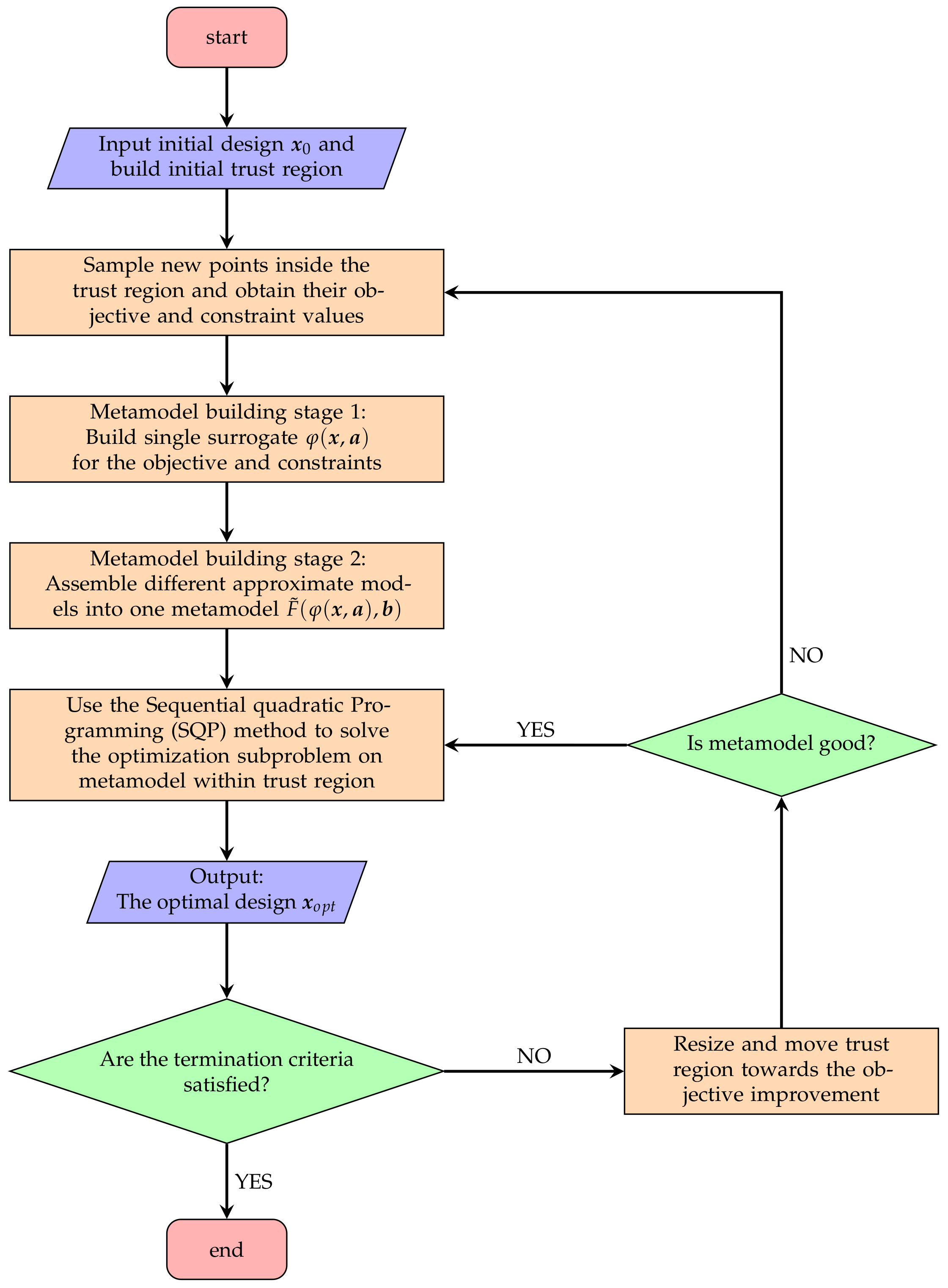
Compared with the time spent by evaluation of the actual response functions $g_j(\mathit{x})$, the selected form of approximate functions ${\tilde{g}}_j^k(\mathit{x}) (j=0,\dots M)$ remarkably reduces the computational expense and adequately improves the accuracy in a current trust region. This is achieved by appropriate planning of numerical experiments and use of the trust region defined by the side constraints $A_i^k$ and $B_i^k$. Once the current suboptimization problem is solved, the suboptimal solution becomes the starting point for the next step. Meanwhile, the move limits are modified and the trust region is resized [25,26]. Based on this information, the metamodel is updated in the next iteration until eventually the optimum is reached.

The process of metamodel building in MAM can be described as an assembly of multiple surrogates into one single metamodel using linear regression. Therefore, there are two stages of metamodel building.

In the first stage, the parameter ${\mathit{a}}_l$ of an individual surrogate ${\phi }_l$ is determined by solving a weighted least squares problem involving n fitting points as

$$min \sum _{i=1}^n{\omega }_i{\left[F({\mathit{x}}_i)-{\phi }_l({\mathit{x}}_i,{\mathit{a}}_l)\right]}^2$$

(3)

where ${\omega }_i$ denotes the weighting parameters and F is the original function that needs to be approximated. Here, the selection of weighting factors ${\omega }_i$ should reflect the quality of the objective function and the location of a design point with respect to the border between the feasible and the infeasible design subspace [30], which are defined as

$$\begin{array}{cc}\hfill w_i& =w_i^o\times w_i^c\hfill \end{array}$$

(4)

$$\begin{array}{cc}\hfill w_i^o& ={\left[\frac{f({\mathit{x}}^k)}{f({\mathit{x}}_i)}\right]}^{\beta }\hfill \end{array}$$

(5)

$$\begin{array}{cc}\hfill w_i^c& =\left\{\begin{array}{cc}1\hfill & \mathrm{for} \mathrm{objective} f(\mathit{x})\hfill \\ {[g(\mathit{x})+1]}^{\alpha }\hfill & \mathrm{if} g(\mathit{x})\le 0\hfill \\ {[g(\mathit{x})+1]}^{-\alpha }\hfill & \mathrm{if} g(\mathit{x})\ge 0\hfill \end{array}\right.\hfill \end{array}$$

(6)

where $\alpha ,\beta >0$ are user-defined constants, where, here, $\alpha =4$ and $\beta =1.5$ are used; ${\mathit{x}}^k$ is the starting point in the kth iteration; and ${\mathit{x}}_i$ is the ith design point in the fitting points. With this definition, a point with a larger objective function has a smaller weighting coefficient component $w_i^o$. For a constraint function $g(\mathit{x})$, a point that is much closer to the boundary of the feasible region of $g(\mathit{x})$ is given a larger weighting coefficient component $w_i^c$. For building a surrogate of the objective function $f(\mathit{x})$, the weighting coefficient $w_i$ only considers the component $w_i^o$. However, for building a surrogate of the constraint function $g(\mathit{x})$, the weighting coefficient $w_i$ will also take the constraint component $w_i^c$ into consideration.

It should be noted here that, in MAM, both the objective and constraint functions will be approximated by Equation (3). The simplest case of ${\phi }_l$ is the first-order polynomial metamodel, and more complex ones are intrinsically linear functions (ILF) that have been successfully applied for solving various design optimization problems [25,28,29]. ILFs are nonlinear but they can be led to linear ones by simple transformations. Currently, five functions are considered in the regressor pool $\left\{{\phi }_l(\mathit{x})\right\}$:

$$\begin{array}{cc}\hfill {\phi }_1(\mathit{x})& =a_0+\sum _{i=1}^N{a}_i{x}_i\hfill \\ \hfill {\phi }_2(\mathit{x})& =a_0+\sum _{i=1}^N{a}_i{x}_i^2\hfill \\ \hfill {\phi }_3(\mathit{x})& =a_0+\sum _{i=1}^N{a}_i/x_i\hfill \\ \hfill {\phi }_4(\mathit{x})& =a_0+\sum _{i=1}^N{a}_i/x_i^2\hfill \\ \hfill {\phi }_5(\mathit{x})& =a_0\prod _{i=1}^N{x}_i^{a_i}\hfill \end{array}$$

(7)

In the second stage, for each function ($f(\mathit{x})$ or $g(\mathit{x})$), different surrogates are assembled into one metamodel:

$$\tilde{F}(\mathit{x})=\sum _{l=1}^{n_l}{b}_l{\phi }_l(\mathit{x})$$

(8)

where $n_l$ is the number of surrogates applied in the model bank $\left\{{\phi }_l(\mathit{x})\right\}$ and $b_l$ is the regression coefficient corresponding to each surrogate ${\phi }_l(\mathit{x})$, which reflects the quality of the individual ${\phi }_l(\mathit{x})$ on the set of validation points. Similar to Equation (3), $b_l$ can be determined in the same manner:

$$min \sum _{i=1}^n{\omega }_i{\left[F({\mathit{x}}_i)-\tilde{F}({\mathit{x}}_i,\mathit{b})\right]}^2$$

(9)

It should be noted that, in the process of metamodel building, the design of experiments (DOE) is fixed, i.e., ${\omega }_i$ remains unchanged across the aforementioned stages.

Figure 1 illustrates the main steps in MAM. Note that, once the metamodels for the objective and constraint functions have been built, the constrained optimization subproblem formulated in the trust region (Equation (2)) could be solved by any existing optimizers. In this paper, the sequential quadratic programming (SQP) method [31] is applied to solve the constrained optimization subproblem for the optimal solution. Since numerical optimization solvers such as SQP are deterministic, the quality of the obtained solution is highly sensitive to the initial point. In other words, MAM could not perform the global search very well. To address this issue, the ASIM framework in Section 4 has been proposed to integrate the stochastic nature with the exploratory search ability of PSO for the global optimal solution.

Figure 1. Flow chart of the mulitpoint approximation method (MAM).

3. Brief Review of Particle Swarm Optimization (PSO)

Particle swarm optimization (PSO), inspired from swarm behaviors in nature such as fish and bird schooling, was developed by Kennedy and Eberhart [32]. Since then, PSO has attracted a lot of attention and been developed as a main representative form of swarm intelligence. PSO has been applied to many areas, such as image and video analysis applications, engineering designs and scheduling applications, classification and data mining, etc. [33]. There are at least twenty PSO variants as well as hybrid algorithms obtained by combining PSO with other existing algorithms, which are also becoming increasingly popular [34,35,36].

To integrate PSO with MAM to find the global optimum, adaptive multi-level search is proposed in this paper. PSO is employed for the global-level exploration in the first step. A number of particles are first placed in the search space of the optimization problem with initial positions and velocities. However, the particles can fly over the entire design space not only determined by the individual and collective knowledge of positions from the global-level search but also based on the “local” information of each particle. Here, the “local” information means the local-level exploitation in the second step. In the neighborhood of each particle, an adaptive metamodel is constructed using MAM in Section 2, which replaces the original optimization problem by a sequence of mathematical approximations that use much simpler objective and constraint functions. Hence, the critical information about individual constraint functions is kept and this leads to the improved accuracy of metamodels. During the process of metamodel building, each particle is endowed with a horizon in the surrounding region and then is refined with the current individual position to boost the possibility of finding an optimal position. Eventually, the swarm as a whole, similar to a flock of birds collectively foraging for food while each bird brilliantly and directly finds the most tasty food within the limited horizon, has the ability to move toward to a global optimum.

Each particle in PSO represents a point in the design space of an optimization problem with an associated velocity vector. In each iteration of PSO, the velocity vector is updated by using a linear combination of three terms shown in Equation (10). The first term called inertia or momentum reflects a memory of the previous flight direction and prevents the particle from changing directions thoroughly. The second term, called the cognitive component, describes the tendency of particles returning to the previously found best positions. The last term, called the social component, quantifies the group norm or standard that should be attained. In other words, each particle tends to move toward the position of the current global best $\mathit{gbest}$ and the location of the individual best $\mathit{pbest}$ while moving randomly [33]. The aim is to find the global best among all the current best solutions until the objective no longer improves or a certain number of iterations are reached. The standard iteration procedure of PSO is formulated as follows:

$$\begin{array}{cc}\hfill {\mathit{V}}_i^{t+1}& =\omega {\mathit{V}}_i^t+\alpha {\mathit{ϵ}}_1({\mathit{pbest}}_i^t-{\mathit{x}}_i^t)+\beta {\mathit{ϵ}}_2({\mathit{gbest}}_i^t-{\mathit{x}}_i^t)\hfill \\ \hfill {\mathit{x}}_i^{t+1}& ={\mathit{x}}_i^t+{\mathit{V}}_i^{t+1}\hfill \end{array}$$

(10)

where $\omega$ is the parameter called inertial weight, t is the current iteration number, $\alpha$ and $\beta$ are parameters called acceleration coefficients, and ${ϵ}_1$ and ${ϵ}_2$ are two homogeneously distributed random vectors generated within the interval $[0,1)$, respectively. If the values of $\omega$, ${ϵ}_1$, and ${ϵ}_2$ are properly chosen ($ϵ=\alpha +\beta >4$ and $\omega =\frac{2}{ϵ-2+\sqrt{{ϵ}^2-4ϵ}}$), it has been proven that PSO could converge to an optimum [37].

Even if PSO has been used in a variety of industry applications, it should be noted that the standard PSO suffers the disadvantages of information loss in the penalty function and high computational cost, especially in solving constrained optimization problems. Therefore, the proposed ASIM framework in the following section takes the advantage of PSO in global searching and reduces the burden on computation by introducing the metamodel building technique, model management, and trust region strategy.

4. Adaptively Integrated Swarm Intelligence-Metamodelling Framework

4.1. Methodology of the ASIM Framework

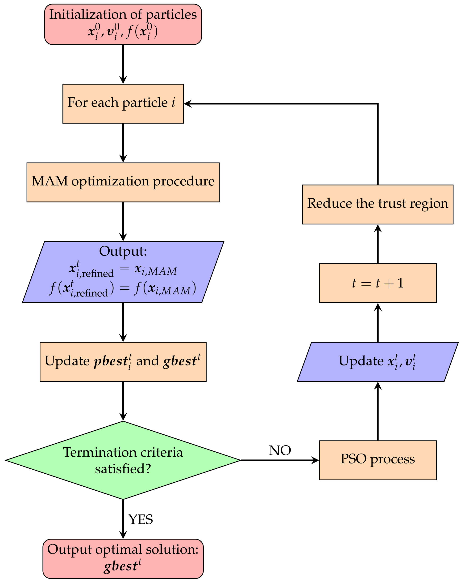
In this paper, an adaptively integrated swarm intelligence-metamodelling (ASIM) framework is proposed to perform a search for the optimal solution in two levels.

In the first level of optimization, also known as exploration, a number of entities are initially placed in the search space of the particular optimization problem with respective positions ${\mathit{x}}_i^t$ and velocities ${\mathbf{\upsilon }}_i^t$. Each particle i has its movement controlled by Equation (10). The final global best solution is obtained only if the objective no longer improves or after a certain number of iterations. However, distinguished from the conventional PSO, each particle also gains an insight within its neighborhood. That forces each particle to refine their personal best position by exploiting their neighborhood, which is known as the second level of optimization. In this local level search, an adaptive metamodel is built by MAM within a trust region surrounding the particle, and then the personal best solution ${\mathit{x}}_{i,MAM}$ obtained by MAM is regarded as a local refinement in position. Following that, the personal and global best position ${\mathit{pbest}}^t,{\mathit{gbest}}^t$ is determined and updated until the termination criterion is satisfied. To sum up, the surrogate helps guide the search direction of each particle and assists in refining the current overall best position until the final global best solution is found. Eventually, the swarm as a whole moves close to a global optimum of the objective function. The flowchart of the ASIM framework is depicted in Figure 2.

Figure 2. Flow chart of ASIM Framework.

It is worth noting that there are three rules applied to compare solutions during the optimization process:

1.

Any feasible solution is preferred to any infeasible solution;

2.

Among feasible solutions, the one with a better objective function value is preferred.

3.

Among infeasible solutions, the one having a fitness value with smaller constraint violations is preferred. In the current implementation, the fitness function is defined by

$$\begin{array}{c}\hfill Fitness(\mathit{x})=\left\{\begin{array}{cc}f(\mathit{x})\hfill & \mathrm{if} \mathit{x} \mathrm{is} \mathrm{feasible}\hfill \\ f(\mathit{x})\times \prod {\left[g_j(\mathit{x})\right]}^2\hfill & \mathrm{elseif} f(\mathit{x})\ge 0\hfill \\ f(\mathit{x})+\left|f(\mathit{x})\right|\times \prod {[g_j(\mathit{x})-1]}^2\hfill & \mathrm{elseif} f(\mathit{x})<0\hfill \end{array}\right.\end{array}$$

(11)

4.2. Model Management

4.2.1. Strategy for Particles “Flying out” in PSO

For particles located outside the boundary, they should adjust their positions according to the formulations determined by the current bounds, as follows:

$$x_{i,k}=\left\{\begin{array}{cc}a\left[k\right]+\gamma \times (b[k]-a[k])\hfill & if x_{i,k}\le a\left[k\right]\hfill \\ b\left[k\right]-\gamma \times (b[k]-a[k])\hfill & if x_{i,k}\ge b\left[k\right]\hfill \end{array}\right.$$

(12)

where $x_{i,k}$ means the kth dimensional position of ${\mathit{x}}_i^t$, $a\left[k\right]$ and $b\left[k\right]$ are kth dimensional side constraints, and $\gamma$ is a relatively small value randomly generated from the range $(0,0.1)$. This perturbation of positions could actually force the particles back into the design space if particles violate the boundary constraints during the entire search process and could ensure the efficiency and accuracy in local exploitation.

4.2.2. Modified Trust Region Strategy in MAM

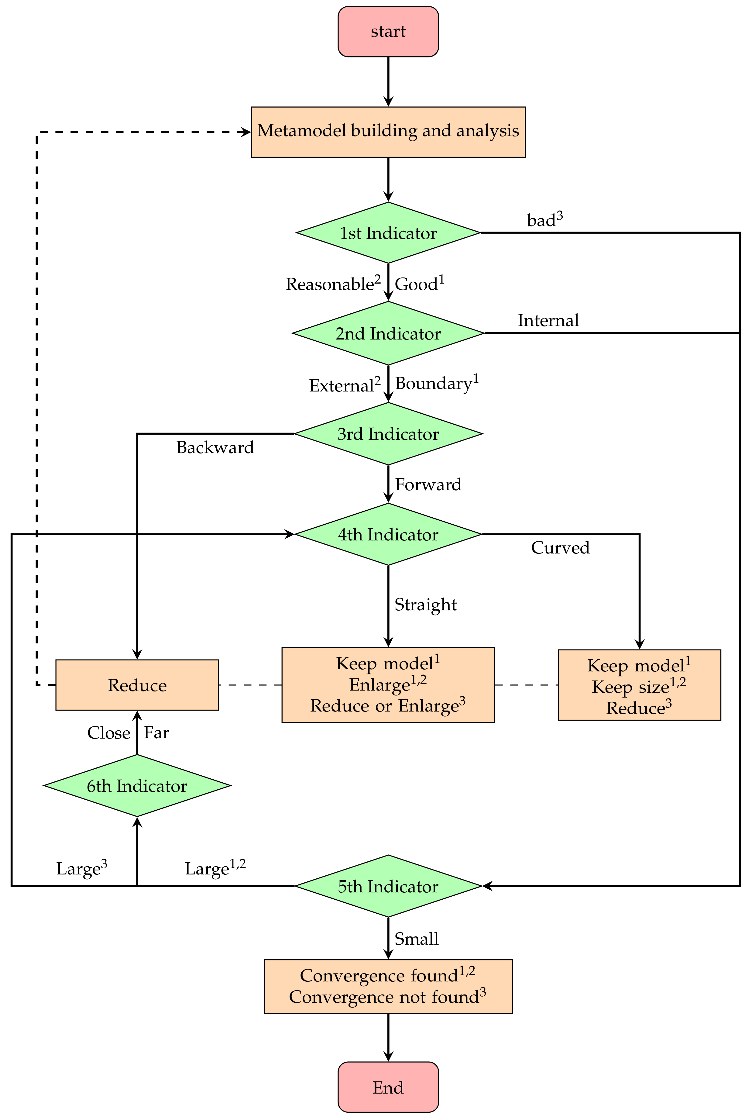
The aim of the trust region strategy in MAM is to control the quality of a metamodel constructed. When the approximation gets better, the trust region is further reduced for the optimal solution. The track of the trust regions also indicates a path of the direction from the initial starting point to the optimum over the entire search domain. At each iteration, a new trust region must be updated, i.e., its new size and its location have to be specified. Several indicators are formulated to support the control of the trust region and to facilitate the search process. The basic knowledge about these indicators was introduced in [38].

The first indicator is to evaluate the quality of the metamodel and focuses on the accuracy of the constraint approximations at the obtained suboptimal point ${\mathit{x}}^{k+1}$. This is based on the following equation:

$$E^k=Ma\mathit{x}\left(|\frac{\tilde{g}\left({\mathit{x}}^{k+1}\right)-g\left({\mathit{x}}^{k+1}\right)}{g\left({\mathit{x}}^{k+1}\right)}|\right)$$

(13)

where $\tilde{g}\left({\mathit{x}}^{k+1}\right)$ and $g\left({\mathit{x}}^{k+1}\right)$ are normalized functions of the approximate and true constraints at the suboptimal point ${\mathit{x}}^{k+1}$, respectively. In this way, a single maximal error quantity between explicit approximation and implicit simulation is defined. Then, the quality of metamodel can be labeled as “bad”, “reasonable”, or “good” shown below.

$$E^k\Rightarrow \left\{\begin{array}{cc}\ge 0.25\times S^k\hfill & \Rightarrow ‘\mathrm{Bad}’\hfill \\ \le 0.01\times S^k\hfill & \Rightarrow ‘\mathrm{Good}’\hfill \\ Else\hfill & \Rightarrow ‘\mathrm{Reasonable}’\hfill \end{array}\right.$$

(14)

where $S^k$ represents the maximum ratio of the dimension length between the present trust region, and the entire design space is defined by

$$S^k=Ma\mathit{x}\left(\frac{B_i^k-A_i^k}{B_i-A_i}\right) (i=1,\dots ,d)$$

(15)

The second indicator is for indicating the location of the current iterate ${\mathit{x}}^{k+1}$ in the present search subregion. For each dimension, if none of the current move limits (${\mathit{A}}^k,{\mathit{B}}^k$) is active, this solution is regarded as “internal”; otherwise, it is viewed as “External”.

The third and fourth indicators reflect the movement history for the entire optimization process. For this purpose, the angle between the last two move vectors is calculated. The formulation of this measure ${\theta }^k$ is given below:

$${\theta }^k=\frac{{\mathit{x}}^{k+1}-{\mathit{x}}^k}{\parallel {\mathit{x}}^{k+1}-{\mathit{x}}^k\parallel }\times \frac{{\mathit{x}}^k-{\mathit{x}}^{k-1}}{\parallel {\mathit{x}}^k-{\mathit{x}}^{k-1}\parallel }$$

(16)

If ${\theta }^k>0$ holds, the movement will be denoted as “forward”, while ${\theta }^k\le 0$ is denoted as moving “backward”. Moreover, if ${\theta }^k\le 0.3$, the convergence history is labelled as “curved”; otherwise, it is “Straight”.

The fifth indicator in MAM, as a termination criterion, is the size of the current search subregion. It can be marked as “small” or “large” according to the quality of the metamodel determined by the first indicator. When the approximations are “bad” and $S^k\le 0.0005$, the present search subregion is considered “small”. When the approximations are “reasonable” or “good”, the trust region is denoted as “small” if $S^k\le 0.001$.

The sixth indicator is based on the most active constraint. It is considered “close” to the boundary between the feasible and infeasible design space if ${\mathit{g}}_{ma\mathit{x}}({\mathit{x}}^{k+1})\in [-0.1,0.1]$; otherwise, it is denoted as “far”.

Both reduction and enlargement of the trust region is executed using

$$B_i^{k+1}-A_i^{k+1}=\frac{1}{\tau }\left(B_i^k-A_i^k\right) \left(i=1,\dots ,d\right)$$

(17)

where $\tau$ is the resizing parameter.

When the approximations are “bad” and the trust region is “small”, the current trust region is considered too small for any further reduction to achieve reasonable approximations and the process is aborted. When the approximations are “bad” and the trust region is “large”, a reduction in the search region should be applied in order to achieve better approximations. When the approximations are not “bad”, the trust region is “large” and the suboptimal point is not “internal”; a “backward” convergence history means that the iteration point progresses in a direction opposite to the previous move vector. In this situation, the trust region has to be reduced. If the iteration point moves “forward” and the approximations are “good”, the same metamodels are reutilized in the next iteration for the purpose of reducing the computational cost. If the optimization convergence history is labelled as “curved” and the approximations are “reasonable”, the trust region is enlarged as the optimization process moves in the same direction.

A summary of termination criteria as well as the move limit strategy is presented in Table 1 and Figure 3, respectively. Note that, in Figure 3, some processes are only executed when the indicators have the same superscript. For example, the process can only output the final optimum when the approximation is “good” (with superscript 1) and the current location (2nd indicator) of the solution is within a small (5th indicator) trust region. If the quality of the metamodel is “bad” with the superscript “3” and the 5th indicator has the value “large”, the 4th indicator is triggered and a move limit should be then determined.

Table 1. Six indicators in MAM.

1st indicator	The quality of metamodel approximation
	Good	Reasonable	Bad
2nd indicator	Location of the suboptimal point ${\mathit{x}}^{k+1}$ with respect to trust region
	Boundary	Internal	External
3rd indicator and 4th indicator	The angle between the last two move vectors
	Backward $\left(\frac{\pi }{2}\le \theta \le \frac{3\pi }{2}\right)$ Parallel		Forward $\left(-\frac{\pi }{2}\le \theta \le \frac{\pi }{2}\right)$ Curved
5th indicator	Termination criterion: size of the current region
	Small		Large
6th indicator	Value of the most active constraint
	Close from the boundary		Far from the boundary

Figure 3. Overview of trust region strategy in MAM.

4.2.3. Space Reduction Scheme in the ASIM Framework

As optimization proceeds, the particles narrow down their horizon to improve the local search ability. In other words, for each particle involved, the size of the individual trust region reduces from $1.0$ by a factor of 2 in each iteration, i.e., ${(\frac{1}{2})}^t$ times the size of the initial design space. Although the particles still fly through the whole design space, each individual seems to behave more cleverly and finds the local optimal position more precisely because the metamodel becomes more accurate.

5. Benchmark Problem

In this section, the parameters used in MAM and the proposed ASIM framework are given in Table 2 for solving complex optimization problems: one benchmark mathematical example and two real-world complex design problems. The MAM parameters (the maximum number of iteration, the number of required sampling points, the size of the initial trust region, and the minimum size of the trust region) are well configured for solving general optimization tasks, as proposed in our previous work [28]. The PSO parameters (the initial weight and the acceleration coefficients) are chosen as the values proposed in [37], which ensure the convergent behavior of the search process.

Table 2. Default parameters for MAM and ASIM.

Method	MAM Parameters				PSO Parameters
	MI a	NOP b	SIR c	SMR d	$\mathit{\omega }$e	$\mathit{\alpha }$f	$\mathit{\beta }$f
MAM	30	$n+5$	0.25	0.1	N.A.
ASIM	30	$n+5$	0.25	0.1	0.7298	1.49618	1.49618

^a The maximum number of iteration. ^b The number of required sampling points. ^c The size of the initial trust region. ^d The minimum size of the trust region. ^e The initial weight in PSO. ^f The acceleration coefficients in PSO.

5.1. Welded Beam

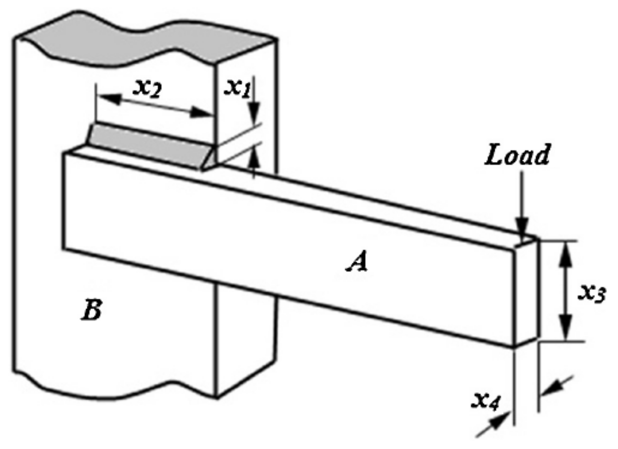
The design optimization of a welded beam in Figure 4 is a complex and challenging problem in nature with many variables and constraints. Usually, conventional optimization methods fail to find global optimal solutions. Hence, the welded beam design problem is often used to evaluate the performance of optimization methods. To determine the best set of design variables for minimizing the total fabrication cost of the structure, the minimum cost optimization is performed considering shear stress $(\tau )$, bending stress $(\sigma )$, buckling load $(p_c)$, and end deflection $\delta$ constraints. The design variables comprise the thickness of the weld $(x_1)$, the length of the welded joint $(x_2)$, the width of the beam $(x_3)$, and the thickness of the beam $(x_4)$, and the mathematical formulation of this problem can be expressed as follows:

$$\begin{array}{cc}\hfill min & f(\mathit{x})=1.10471x_1^2{x}_2+0.04811x_3{x}_4(14+x_2)\hfill \\ \hfill s.t. & g_1(\mathit{x})=\tau (\mathit{x})-{\tau }_{max}\le 0\hfill \\ \hfill & g_2(\mathit{x})=\sigma (\mathit{x})-{\sigma }_{max}\le 0\hfill \\ \hfill & g_3(\mathit{x})=x_1-x_4\le 0\hfill \\ \hfill & g_4(\mathit{x})=[0.10471x_1^2+0.04811x_3{x}_4(14+x_2)]-5\le 0\hfill \\ \hfill & g_5(\mathit{x})=0.125-x_1\le 0\hfill \\ \hfill & g_6(\mathit{x})=\delta (\mathit{x})-{\delta }_{max}\le 0\hfill \\ \hfill & g_7(\mathit{x})=p-p_c(\mathit{x})\le 0\hfill \\ \hfill where & P=6000 lb, L=14 in, E=30\times {10}^6 psi, G=12\times {10}^6 psi,\hfill \\ \hfill & {\tau }_{max}=13,600 psi, {\sigma }_{max}=30,000 psi, {\delta }_{max}=0.25 in\hfill \\ \hfill & {\tau }^{\prime }=\frac{P}{\sqrt{2}{x}_1{x}_2},{\tau }^{″}=\frac{MR}{J},M=P\left(L+\frac{x_2}{2}\right)\hfill \\ \hfill & R=\sqrt{\frac{x_2^2}{4}+{\left(\frac{x_1+x_3}{2}\right)}^2}\hfill \\ \hfill & \tau (x)=\sqrt{{\left({\tau }^{\prime }\right)}^2+2{\tau }^{\prime }{{\tau }^{″}}^{\frac{x_2}{2R}}+{\left({\tau }^{″}\right)}^2}\hfill \\ \hfill & J=2\left\{\sqrt{2}{x}_1{x}_2\left[\frac{x_2^2}{12}+{\left(\frac{x_1+x_3}{2}\right)}^2\right]\right\}\hfill \\ \hfill & \sigma (x)=\frac{6PL}{x_4{x}_3^2},\delta (x)=\frac{4P{L}^3}{E{x}_3^3{x}_4}\hfill \\ \hfill & p_c(x)=\frac{4.013\sqrt{E\left(\frac{x_3^2{x}_4^6}{36}\right)}}{L^2}\left(1-\frac{x_3}{2L}\sqrt{\frac{E}{4G}}\right)\hfill \\ \hfill & 0.1\le x_1\le 2, 0.1\le x_2\le 10, 0.1\le x_3\le 10, 0.1\le x_4\le 2\hfill \end{array}$$

(18)

Figure 4. Schematic of the welded beam structure with indication of design variables.

To solve the aforementioned problem, the GA-based method [39], co-evolutionary PSO method (CPSO) [22], ES-based method [40], charged system search (CSS) [41], and colliding bodies optimization (CBO) [42] were used to find the optimal solution.

In Table 3, the optimized design variables and cost obtained by MAM and ASIM have been compared with those obtained in literature. The best solutions ($1.724852$) by MAM and ASIM are more competitive than those obtained by other methods. Although Kaveh [42] claimed that $1.724663$ was the better cost, the solution actually violated the $g_1$ constraint and it was an infeasible solution. Based on the statistical results in Table 4, it is concluded that the ASIM technique is very robust and efficient because the standard deviation of different runs of simulations is almost 0 ($1.1\times {10}^{-7}$) and the number of function analysis (NFEs) is remarkably smaller (565) than that called by other methods except MAM. Both ASIM and MAM demonstrate efficiency in finding the optimal design owing to their accuracy approximations and adaptive trust region strategy at local level exploitation. On average, hundreds of evaluations are required to determine an optimum. It is noted that enhancement of global exploration for the optimal solution by the PSO process in the ASIM framework could be demonstrated by a standard deviation of zero ($1.1\times {10}^{-7}$) for statistical results, which is approximately four orders of magnitude smaller than the value by MAM (0.0031358). Furthermore, by comparison with the NFEs (200,000) obtained by co-evolutionary PSO [22], the accurate surrogates built by ASIM framework indeed assist each particle in finding the local refinement position and speed up the converged global optimum. In conclusion, ASIM needs less computational cost for a global optimum with improved accuracy and great robustness.

Table 3. Comparison of present optimized designs with the literature for welded beams.

Methods	${\mathit{x}}_1\left(\mathit{h}\right)$	${\mathit{x}}_2\left(\mathit{l}\right)$	${\mathit{x}}_3\left(\mathit{t}\right)$	${\mathit{x}}_4\left(\mathit{b}\right)$	Cost
GA-based [39]	0.205986	3.471328	9.020224	0.20648	1.728226
CPSO [22]	0.202369	3.544214	9.04821	0.205723	1.728024
ES-based [40]	0.199742	3.612060	9.037500	0.206082	1.737300
CSS [41]	0.20582	3.468109	9.038024	0.205723	1.724866
CBO [42]	0.205722	3.47041	9.037276	0.205735	1.724663
MAM	0.2057296	3.4704893	9.0366242	0.2057297	1.724852
ASIM	0.2057296	3.4704887	9.0366239	0.2057296	1.724852

Table 4. Statistical results from different optimization methods for the welded beam design problem.

Methods	Best	Average	Worst	S.D.	NFEs
GA-based [39]	1.728226	1.792654	1.993408	0.074713	80000
CPSO [22]	1.728024	1.748831	1.782143	0.012926	200000
ES-based [40]	1.737300	1.813290	1.994651	0.070500	25,000
CSS  [41]	1.724866	1.739654	1.759479	0.008064	4000
CBO  [42]	1.724662	1.725707	1.725059	0.0002437	4000
MAM	1.724852	1.725563	1.739605	0.0031358	122
ASIM	1.724852	1.724852	1.724852	1.10E-07	565

5.2. Design of a Tension/Compression Spring

This problem, first described by Belegundu [43], has arisen from the wide applications of vibration resistant structures in civil engineering. The design objective is to minimize the weight of a tension/compression spring subject to constraints on the minimum deflection $g_1$, shear stress $g_2$, and surge frequency $g_3$ and to limit on the outside diameter $g_4$. As shown in Figure 5, the design variables include the wire diameter d, the mean coil diameter D, and the number of active coils N. The mathematical description of this problem can be expressed as follows:

$$\begin{array}{cc}\hfill min & f\left(N, D, d\right)=\left(N+2\right)\times D{d}^2\hfill \\ \hfill s.t. & g_1(\mathit{x})=1-\frac{D^{3}N}{71,785d^4}\le 0\hfill \\ \hfill & g_2(\mathit{x})=\frac{4D^2-Dd}{12,566\left(D{d}^3-d^4\right)}+\frac{1}{5108d^2}-1\le 0\hfill \\ \hfill & g_3(\mathit{x})=1-\frac{140.45d}{D^{2}N}\le 0\hfill \\ \hfill & g_4(\mathit{x})=\frac{D+d}{1.5}-1\le 0\hfill \\ \hfill \mathrm{where} & 0.05\le d\le 1, 0.25\le D\le 1.3, 2\le N\le 15.\hfill \end{array}$$

(19)

Figure 5. Schematic of the tension/compression spring.

The statistical results by MAM are in Table 5. From the first row to the sixth row, every row is the optimal results of 40 independent runs of MAM and the last line concludes the average results of the 6 parallel experiments, i.e., each experiment comprises 40 independent runs of MAM with randomly generated starting points. The best optimal design represented by $[d,D,N]$ is [0.051656122, 0.355902943, 11.33791803] with the objective value of $0.012666692$. Moreover, the fourth column “Best” in Table 5 indicates that MAM cannot achieve a converged robust solution and falls into the local optima when faced with multimodal function optimization. The optimal result ranges from $0.01266$ (the best design in the fourth row) to $0.070$ (the worst design in the third row). As a general deficiency of the trajectory-based algorithm, MAM could not find the known optimum $0.0126652$ by balancing the efforts between exploration and exploitation.

Table 5. Statistical results for the tension/compression spring problem by MAM.

Number	Worst	Mean	Best	S.D.	NFEsa
1	0.032839737	0.015057587	0.0126692	0.004246608	8041
2	0.046478999	0.01537479	0.012677425	0.005275199	8536
3	0.070551755	0.015521846	0.012680762	0.009064574	7483
4	0.053871312	0.016530777	0.012666692	0.00857695	7483
5	0.030829567	0.014687079	0.012733211	0.003455907	7536
6	0.017557055	0.014067046	0.012667273	0.001247161	8149
Average	0.012733211	0.012682427	0.012666692	$2.55305\times {10}^{-5}$	7871

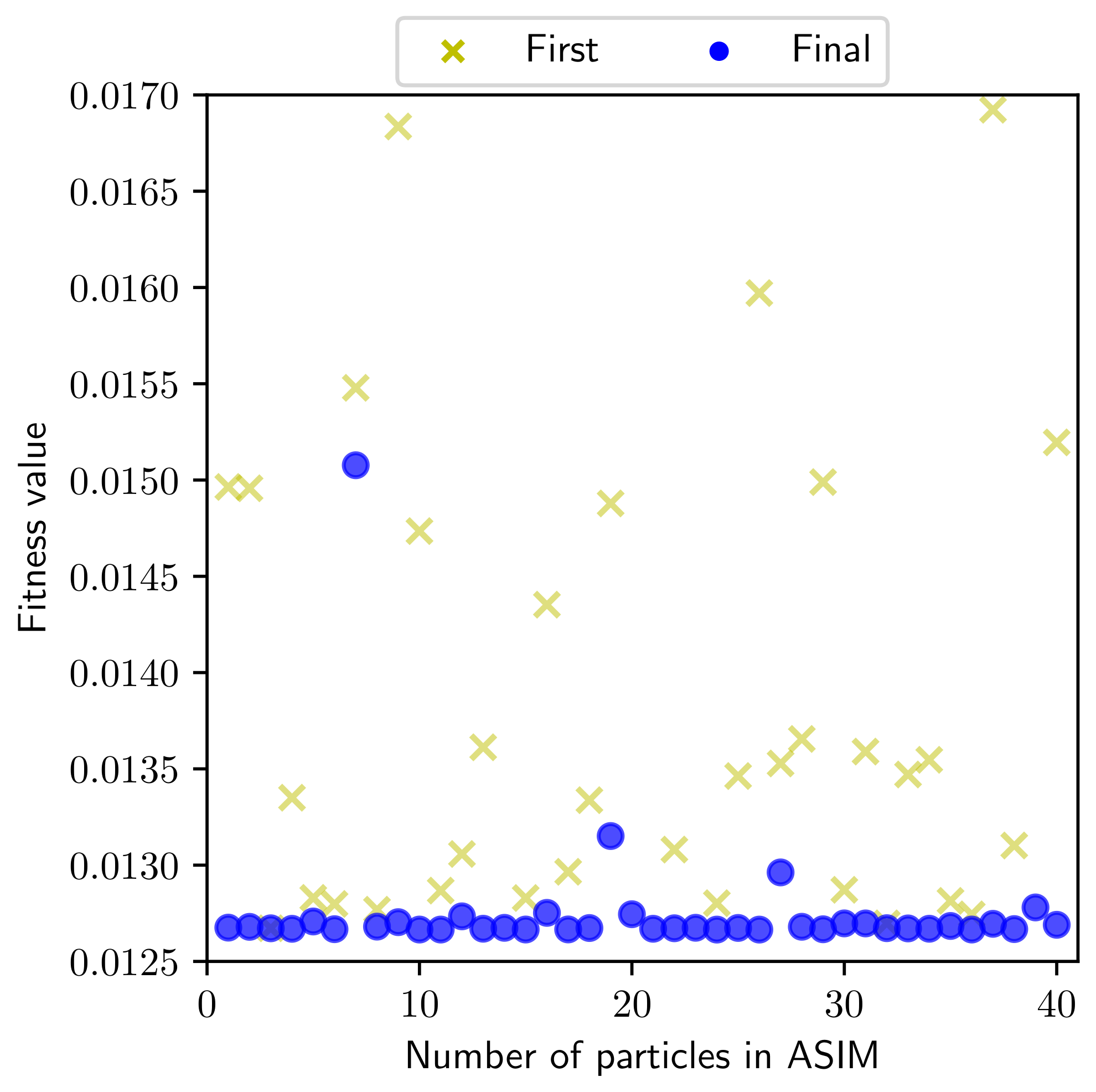
A more intuitive perspective for understanding the global search mechanism using the ASIM framework is represented in Table 6, which includes the optimal results obtained by 8 independent experiments, each of which is initialized with 5 particles. In Figure 6, the results show the objectives of initial designs and global optima for the tested 40 particles. Even the initial designs are remarkably different at the start of the optimization process due to the random nature of statistical tests; the developed ASIM has the capability to eventually find the converged global optimum. It is concluded that the ASIM algorithm can achieve a robust solution for random starting points, and it will not be trapped into local optima due to its multi-level search and model management strategies. Therefore, these 8 independent experiments could almost obtain the same global optimum. The best optimal design found by ASIM framework is $[0.051724501,0.357570887,11.23912608]$, with the objective value $0.012665259$, which has a good agreement with the known optimum. Additionally, the global solutions from 8 independent experiments have been proven feasible by function evaluations.

Table 6. Statistical results for the tension/compression spring problem by adaptively integrated swarm intelligence-metamodelling (ASIM).

Number	Worst	Mean	Best	S.D.	NFEs
1	0.012707419	0.01268076	0.012669372	$1.53792\times {10}^{-5}$	4891
2	0.015076822	0.013158868	0.012665512	0.001072278	5719
3	0.012734131	0.012681909	0.012665469	$2.94215\times {10}^{-5}$	5161
4	0.013151181	0.012797596	0.012666127	0.000201587	5233
5	0.012674725	0.012671127	0.012665294	$3.80784\times {10}^{-6}$	4882
6	0.012962267	0.012734387	0.012665259	0.000128041	5337
7	0.012787169	0.012679022	0.012669651	$1.17008\times {10}^{-5}$	4702
8	0.012780362	0.01269988	0.012665634	$4.68624\times {10}^{-5}$	5170
Average	0.012669651	0.01266654	0.012665259	$1.85492\times {10}^{-6}$	5141

Figure 6. First and final fitness values in ASIM for solving the tension/compression spring.

Other algorithms recently used to optimize this problem include co-evolutionary particle swarm optimization (CPSO) [22], differential evolution with dynamic stochastic selection (DEDS) [44], hybrid evolutionary algorithm with adaptive constraint-handling techniques (HEAA) [45], league championship algorithm (LCA) [46], water cycle algorithm (WCA) [24], and hybrid cuckoo search (HCS) [23]. A comparison of the optimal solutions by the aforementioned methods is given in Table 7, and the statistical results by ASIM, MAM, and other algorithms are shown in Table 8.

Table 7. Comparison of the best solutions obtained by various studies for the tension/compression spring design optimization problem.

Name	CPSO [22]	DEDS [44]	HEAA [45]	LCA [46]	WCA [24]	HCS [23]	MAM	ASIM
$x_1$	0.051728	0.051689	0.051689	0.051689	0.051680	0.051689	0.051656	0.051724
$x_2$	0.357644	0.356717	0.356729	0.356718	0.356522	0.356718	0.355902	0.357570
$x_3$	11.244543	11.288965	11.288293	11.28896	11.300410	11.28896	11.33791	11.239126
$g_1(x)$	$-8.25\times {10}^{-4}$	$1.45\times {10}^{-9}$	$3.96\times {10}^{-10}$	N.A./$2.00\times {10}^{-15}$	$-1.65\times {10}^{-13}$	$-6.41\times {10}^{-6}$	$-1.64\times {10}^{-5}$	$-1.13\times {10}^{-7}$
$g_2(x)$	$-2.52\times {10}^{-5}$	$-1.19\times {10}^{-9}$	$-3.59\times {10}^{-10}$	N.A./$-2.22\times {10}^{-15}$	$-7.9\times {10}^{-14}$	$-3.90\times {10}^{-6}$	$-5.16\times {10}^{-5}$	$-1.05\times {10}^{-7}$
$g_3(x)$	−4.051306	−4.053785	−4.053808	N.A./−4.053786	−4.053399	−4.053775	$-4.051810$	$-4.055466$
$g_4(x)$	−0.727085	−0.727728	−0.727720	N.A./−0.727728	−0.727864	−0.727729	$-0.728293$	$-0.727136$
$f(x)$	0.012674	0.012665	0.012665	0.01266523	0.012665	0.0126652	0.0126667	0.0126652

Table 8. Comparison of statistical results given by different algorithms for the tension/compression spring design optimization problem.

Methods	Worst	Mean	Best	S.D.	NFEs
CPSO [22]	0.012924	0.012730	0.012674	$5.20\times {10}^{-4}$	240,000
DEDS [44]	0.012738	0.012669	0.012665	$1.3\times {10}^{-5}$	24,000
HEAA [45]	0.012665	0.012665	0.012665	$1.4\times {10}^{-9}$	24,000
LCA [46]	0.01266667	0.01266541	0.01266523	$3.88\times {10}^{-7}$	15,000
WCA [24]	0.012952	0.012746	0.012665	$8.06\times {10}^{-5}$	11,750
HCS [23]	0.0126764	0.0126683	0.0126652	$5.37\times {10}^{-7}$	150,000
MAM	0.012733211	0.012682427	0.012666692	$2.55305\times {10}^{-5}$	7871
ASIM	0.012669651	0.01266654	0.012665259	$1.85492\times {10}^{-6}$	5141

In Table 7, the ASIM framework has the ability to find the optimal solution (0.0126652), which is the best available design compared to that which the other algorithms achieved. Although LCA [46] found a slighter better solution (0.01266523), the corresponding constraint $g_1(\mathit{x})$ was violated. Therefore, it was not a feasible solution. The same conclusion can be drawn for the results by DEDS [44] and HEAA [45]. Together with the statistical results shown in Table 8, it can be observed that the ASIM method is superior to other methods for the global solution in terms of the number of function evaluations and the accuracy throughout the optimization process. Obviously, the referenced methods used more than 10,000 calls to find the global optimum while ASIM finds the optimum with about half of those calls. Meanwhile, the ASIM could reduce the number of simulations by over $28\%$ compared to MAM.

As a general remark on the comparisons above, ASIM shows a very competitive performance over eight state-of-the-art optimization methods to find the global optimal solution in terms of the efficiency, the quality, and the robustness.

5.3. Mathematical Problem G10

This problem was first described in [47] and then was considered one of the benchmark problems at the 2006 IEEE Congress on Evolutionary Computation [48]. In this optimization example, there are eight variables and six inequality constraints (three linear and three nonlinear). The mathematical formulations are shown below.

$$\begin{array}{cc}\hfill min & f(\mathit{x})=x_1+x_2+x_3\hfill \\ \hfill s.t. & g_1(\mathit{x})=-1+0.0025(x_4+x_6)\le 0\hfill \\ \hfill & g_2(\mathit{x})=-1+0.0025(x_5+x_7-x_4)\le 0\hfill \\ \hfill & g_3(\mathit{x})=-1+0.01(x_8-x_5)\le 0\hfill \\ \hfill & g_4(\mathit{x})=-x_1{x}_6+833.33252x_4+100x_1-83,333.333\le 0\hfill \\ \hfill & g_5(\mathit{x})=-x_2{x}_7+1250x_5+x_2{x}_4-1250x_4\le 0\hfill \\ \hfill & g_6(\mathit{x})=-x_3{x}_8+1,250,000+x_3{x}_5-2500x_5\le 0\hfill \\ \hfill \mathrm{where} & 100\le x_1\le 10,000,1000\le x_i\le 10,000(i=2, 3),\hfill \\ \hfill & 10\le x_i\le 1000(i=4,\dots , 8)\hfill \end{array}$$

(20)

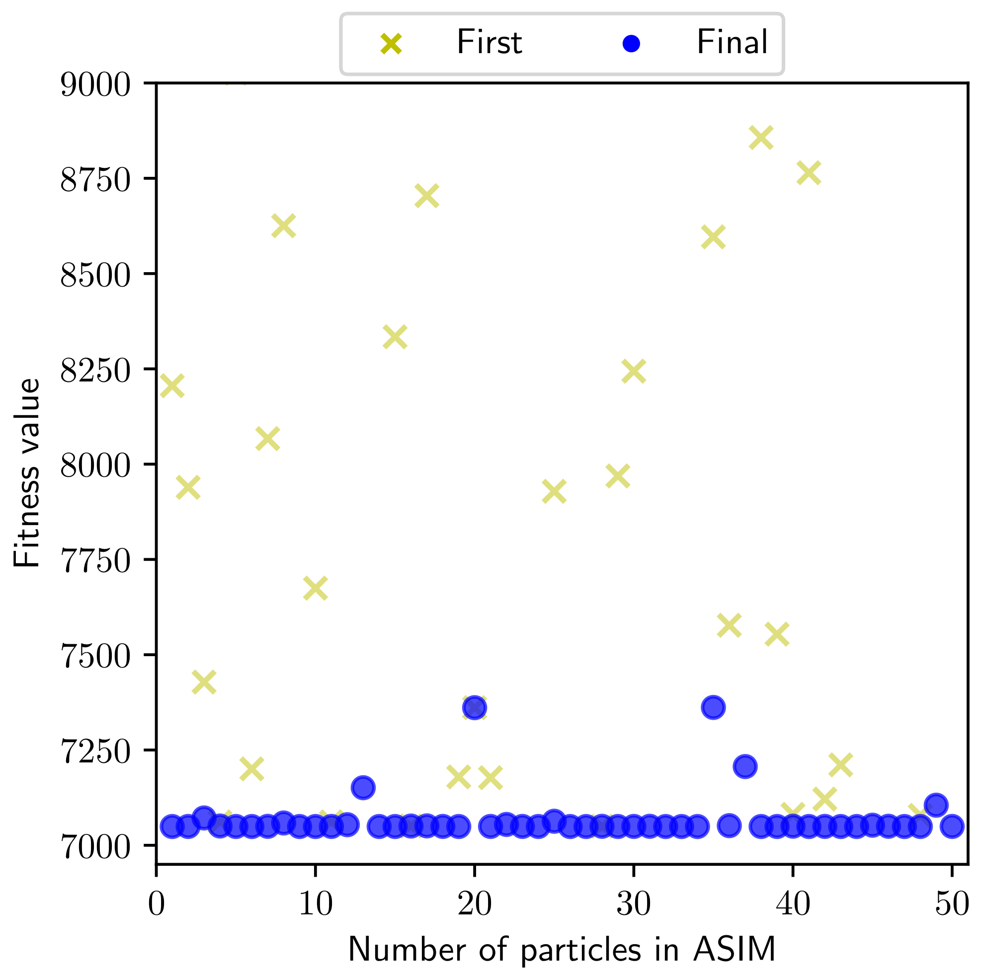
The optimal solutions found by ASIM and MAM are given in Table 9 as well as the known optimum. In Table 10, nine independent experiments have been performed and each experiment includes 40 parallel runs of MAM. Although each run by MAM is initialized with a random starting point, there is no guarantee that the converged global optimum can be achieved. As there has a very small feasible region $(0.0010\%)$ in this challenging example, limited runs by MAM could not find a feasible solution, and normally, a bad design with a very large value of the fitness function (up to 100,000) is obtained. However, a feasible solution could be achieved within 20,000 function evaluations. Applying the developed ASIM, the capability of the adaptive multi-level search for the global optimum was significantly improved, and the statistical results are shown in Table 11. Using the same parameter settings in the previous example, the worst solution found by the particles is about 7361, which is only $4.42\%$ higher than the global optimum $7049.248$. In the mean time, all nine independent experiments of ASIM could find a decent global optimum, which is slightly ${10}^{-5}$ higher than the global optimum even in the worst case (number 5 in Table 11). In Figure 7, it shows how 10 independent runs initialized with a total of 50 particles converge to the global optimum by ASIM. It is noted that the initial design varies dramatically for each particle, and finally, all particles succeed in finding the global optimum. It is concluded that the PSO process applied in ASIM remarkably boosts the exploration capability. Owing to advantages such as the guidance of personal memory for the best position and social cognition in addition to the stochastic search behavior, ASIM is a robust and efficient algorithm for solving such a challenging problem.

Table 9. Optimal solutions of G10 found by ASIM and MAM.

Description	Solution $[{\mathit{x}}_1,{\mathit{x}}_2,{\mathit{x}}_3,{\mathit{x}}_4,{\mathit{x}}_5,{\mathit{x}}_6,{\mathit{x}}_7,{\mathit{x}}_8]$	Objective Value
Known optimum [48]	[579.3066850, 1359.9706780, 5109.970657, 182.0176996, 295.6011737, 217.98230036, 286.4165259, 395.6011737]	7049.2480
ASIM	[579.0697378, 1360.029849, 5110.148583, 181.9979046, 295.5940579, 218.0020914, 286.4038427, 395.5940579]	7049.2481
MAM	[579.2439615, 1360.814966, 5109.189094, 182.0124631, 295.6324343, 217.9875329,286.380036, 395.6324333]	7049.2499

Table 10. Statistical results for G10 by MAM.

Number	Worst	Mean	Best	S.D.	NFEs
1	142,392.7156	17,882.82055	7069.390888	30,251.49815	18,436
2	68,065.07371	11,619.11583	7049.296446	11,320.46339	19,388
3	43,458.18348	10,426.99053	7049.249948	6247.162418	19,584
4	76,953.38912	12,669.27407	7052.442664	12,331.32358	18,478
5	53,761.55465	11,938.01326	7060.468503	8513.607171	19,122
6	38,601.51929	11,216.42827	7049.304236	5669.873504	17,274
7	133,020.3445	12,395.33809	7062.698763	19,714.98684	19,640
8	50,195.68872	12,527.61721	7061.831868	10,079.5634	19,668
9	86,553.78422	12,382.57366	7053.509331	13,257.22511	20,270
Average	7069.390888	7056.46585	7049.249948	7.334903947	19,095

Table 11. Statistical results for G10 by ASIM.

Number	Worst	Mean	Best	S.D.	NFEs
1	7071.746167	7054.064714	7049.24996	9.89925027	19,374
2	7058.554639	7051.206052	7049.248851	4.112416516	20,452
3	7151.048877	7070.606275	7049.248909	45.01472868	19,612
4	7361.05089	7112.256788	7049.275307	139.0818573	18,450
5	7063.107951	7053.22295	7049.318392	5.982378418	19,094
6	7049.802007	7049.418117	7049.248849	0.23813293	19,318
7	7361.648467	7111.850254	7049.248177	139.6416717	20,102
8	7206.603344	7081.369993	7049.26296	70.01358744	19,780
9	7052.697369	7049.999679	7049.251224	1.512797685	19,962
10	7105.192042	7060.643287	7049.261412	24.90483007	19,794
Average	7049.318392	7049.262676	7049.248177	0.024517331	19,522

Figure 7. First and final output fitness values for G10 in a hybrid optimization framework.

Recently, other algorithms including evolutionary optimization by approximate ranking and surrogate models (EOAS) [49], constraint optimization via particle swarm optimization (COPSO) [50], league championship algorithm (LCA) [46], hybrid cuckoo search (HCS) [23], and surrogate-assisted differential evolution (SADE) [51] have also solved this optimization problem. A comparison of results by ASIM, MAM, and other algorithms is given in Table 12. Although all methods listed are very competitive and has the ability to find global or near global optimum, ASIM demonstrates superiority over the others in terms of computational efficiency. Evolutionary algorithms usually need over 150,000 simulations to find the global optimum, while ASIM could reduce the number of function evaluations to 19,522 by more than $80\%$. Furthermore, the optimum $(7049.2481)$ achieved by ASIM is in a good agreement with the global optimum $(7049.2480)$. Although HCS [23] proposed a best optimum ($7049.237$), the fourth constraint is slightly violated and, therefore, is not a feasible design. Summarily, ASIM outperforms other methods in seeking the global optimal solutions of complex black-box optimization problems in terms of efficiency and accuracy.

Table 12. Statistical features of the results obtained by various algorithms on G10.

Methods	Worst	Mean	Best	S.D.	NFEs
EOAS [49]	7258.540	7082.227	7049.404	42.0	304,066
COPSO [50]	7049.668593	7049.278821	7049.248871	N.A.	240,000
LCA [46]	7049.2482816	7049.2480542	7049.2480206	$5.80\times {10}^{-5}$	225,000
HCS [23]	7250.957	7049.668	7049.237	86.5	150,000
SADE [51]	N.A.	7278.785	7049.249	N.A.	500,000
MAM	7069.390888	7056.46585	7049.249948	7.334903947	19,095
ASIM	7049.318392	7049.262676	7049.248177	0.024517331	19,522

6. Conclusions

In this paper, an adaptively integrated swarm intelligence-metamodelling (ASIM) technique that enables adaptive multi-level adaptive search for the global optimal solution was proposed for solving expensive and complex black-box constrained optimization problems. In the first step, the adaptive swarm-intelligence algorithm carries out global exploration for the near-optimal solution. In the second step, the metamodel-based optimization algorithm multipoint approximation method (MAM) is performed for local exploitation. Essentially, each particle’s current position in ASIM gains local refinement by optimization of metamodel building around their neighborhood and tends to move towards the global best position according to swarm intelligence. Eventually, the swarm as a whole, similar to a flock of birds collectively foraging for food while each bird brilliantly finds the most tasty food with limited horizon directly, possibly moves close to a global optimum position. One mathematical problem and two engineering optimization problems were studied in detail using the ASIM framework. By comparison of the results obtained from ASIM, MAM, and other state-of-art algorithms, it was demonstrated that ASIM has the capability to tackle expensive constrained black-box optimization problems with remarkably less computational effort, higher accuracy, and stronger robustness. The adaptive multi-level search ability of ASIM indeed makes up the local search deficiency and the sensitivity to the starting point observed in MAM. Consequently, the ASIM technique achieves a good balance between exploration and exploitation. Moreover, ASIM provides valuable insight into the development of nature-inspired metaheuristic algorithms for solving nonlinear optimization problems with less computational cost throughout the simulation-based optimization process.

References

1. Hickernell, F.J.; Yuan, Y.X. A Simple Multistart Algorithm for Global Optimization. OR Trans. 1997, 1, 1–12. [Google Scholar]
2. Rios, L.M.; Sahinidis, N.V. Derivative-free optimization: A review of algorithms and comparison of software implementations. J. Glob. Optim. 2013, 56, 1247–1293. [Google Scholar] [CrossRef] [Green Version]
3. Glover, F. Future paths for integer programming and links to artficial intelligence. Comput. Oper. Res. 1986, 13, 533–549. [Google Scholar] [CrossRef]
4. Kirkpatrick, S.; Gelatt, C.D., Jr.; Vecchi, M.P. Optim. Simulated Annealing. Science 1983, 220, 671–680. [Google Scholar] [CrossRef] [PubMed]
5. Holland, J.H. Adaptation in Natural and Artificial Systems: An introductory Analysis with Applications to Biology, Control and Artificial Intelligence; MIT Press: Cambridge, MA, USA, 1975; p. 183. [Google Scholar] [CrossRef]
6. Borowska, B. Genetic Learning Particle Swarm Optimization with Interlaced Ring Topology. In Computational Science—ICCS 2020; Krzhizhanovskaya, V.V., Závodszky, G., Lees, M.H., Dongarra, J.J., Sloot, P.M.A., Brissos, S., Teixeira, J., Eds.; Springer International Publishing: Cham, Switzerland, 2020; pp. 136–184. [Google Scholar]
7. Wang, S.; Liu, G.; Gao, M.; Cao, S.; Guo, A.; Wang, J. Heterogeneous Comprehensive Learning and Dynamic Multi-Swarm Particle Swarm Optimizer with Two Mutation Operators; Elsevier Inc.: Amsterdam, The Netherlands, 2020; Volume 540, pp. 175–201. [Google Scholar] [CrossRef]
8. Ahmad, R.; Choubey, N.S. Review on Image Enhancement Techniques Using Biologically Inspired Artificial Bee Colony Algorithms and Its Variants. In Biologically Rationalized Computing Techniques for Image Processing Applications; Hemanth, J., Emilia, B.V., Eds.; Springer International Publishing: Cham, Switzerland, 2018; pp. 249–271. [Google Scholar] [CrossRef]
9. Acevedo, H.G.S.; Escobar, C.M.; Andres Gonzalez-Estrada, O. Damage detection in a unidimensional truss using the firefly optimization algorithm and finite elements. arXiv 2018, arXiv:1706.04449. [Google Scholar]
10. Mortazavi, A.; Togan, V. Sizing and layout design of truss structures under dynamic and static constraints with an integrated particle swarm optimization algorithm. Appl. Soft Comput. 2016, 51, 239–252. [Google Scholar] [CrossRef]
11. soon Ong, Y.; Nair, P.B.; Keane, A.J.; Wong, K.W. Surrogate-Assisted Evolutionary Optimization Frameworks for High-Fidelity Engineering Design Problems. In Knowledge Incorporation in Evolutionary Computation; Yaochu, J., Ed.; Springer: Berlin, Germany, 2005; pp. 307–331. [Google Scholar] [CrossRef] [Green Version]
12. Kleijnen, J.P. Kriging metamodeling in simulation: A review. Eur. J. Oper. Res. 2009, 192, 707–716. [Google Scholar] [CrossRef] [Green Version]
13. Myers, R.H.; Montgomery, D.T.; Vining, G.G.; Borror, C.M.; Kowalski, S.M. Response Surface Methodology: A Retrospective and Literature Survey. J. Qual. Technol. 2004, 36, 53–78. [Google Scholar] [CrossRef]
14. Dyn, N.; Levin, D.; Rippa, S. Numerical procedures for surface fitting of scattered data by radial functions. SIAM J. Sci. Stat. Comput. 1986, 7, 639–659. [Google Scholar] [CrossRef]
15. Gerrard, C.E.; McCall, J.; Coghill, G.M.; Macleod, C. Exploring aspects of cell intelligence with artificial reaction networks. Soft Comput. 2014, 18, 1899–1912. [Google Scholar] [CrossRef]
16. Dong, H.; Song, B.; Dong, Z.; Wang, P. SCGOSR: Surrogate-based constrained global optimization using space reduction. Appl. Soft Comput. J. 2018, 65, 462–477. [Google Scholar] [CrossRef]
17. Zhou, Z.; Ong, Y.S.; Nair, P.B.; Keane, A.J.; Lum, K.Y. Combining Global and Local Surrogate Models to Accelerate Evolutionary Optimization. IEEE Trans. Syst. Man Cybern. Part C Appl. Rev. 2007, 37, 66–76. [Google Scholar] [CrossRef] [Green Version]
18. Regis, R.G. Evolutionary Programming for High-Dimensional Constrained Expensive Black-Box Optimization Using Radial Basis Functions. IEEE Trans. Evol. Comput. 2014, 18, 326–347. [Google Scholar] [CrossRef]
19. Bouhlel, M.A.; Bartoli, N.; Regis, R.G.; Morlier, J.; Regis, R.G.; Otsmane, A. Efficient global optimization for high-dimensional constrained problems by using the Kriging models combined with the partial least squares method. Eng. Optim. 2018, 50, 2038–2053. [Google Scholar] [CrossRef]
20. Tang, Y.; Chen, J.; Wei, J. A surrogate-based particle swarm optimization algorithm for solving optimization problems with expensive black box functions. Eng. Optim. 2013, 45, 557–576. [Google Scholar] [CrossRef]
21. Regis, R.G. Particle swarm with radial basis function surrogates for expensive black-box optimization. J. Comput. Sci. 2014, 5, 12–23. [Google Scholar] [CrossRef]
22. He, Q.; Wang, L. An effective co-evolutionary particle swarm optimization for constrained engineering design problems. Eng. Appl. Artif. Intell. 2007, 20, 89–99. [Google Scholar] [CrossRef]
23. Long, W.; Liang, X.; Huang, Y.; Chen, Y. An effective hybrid cuckoo search algorithm for constrained global optimization. Neural Comput. Appl. 2014, 25, 911–926. [Google Scholar] [CrossRef]
24. Eskandar, H.; Sadollah, A.; Bahreininejad, A.; Hamdi, M. Water cycle algorithm—A novel metaheuristic optimization method for solving constrained engineering optimization problems. Comput. Struct. 2012, 110–111, 151–166. [Google Scholar] [CrossRef]
25. Toropov, V.V.; Filatov, A.A.; Polynkin, A.A. Multiparameter structural optimization using FEM and multipoint explicit approximations. Struct. Optim. 1993, 6, 7–14. [Google Scholar] [CrossRef]
26. Keulen, F.V.; Toropov, V.V. New Developments in Structural Optimization Using Adaptive Mesh Refinement and Multipoint Approximations. Eng. Optim. 1997, 29, 217–234. [Google Scholar] [CrossRef]
27. Polynkin, A.; Toropov, V.V. Mid-range metamodel assembly building based on linear regression for large scale optimization problems. Struct. Multidiscip. Optim. 2012, 45, 515–527. [Google Scholar] [CrossRef]
28. Liu, D.; Toropov, V.V. Implementation of Discrete Capability into the Enhanced Multipoint Approximation Method for Solving Mixed Integer-Continuous Optimization Problems. Int. J. Comput. Methods Eng. Sci. Mech. 2016, 17. [Google Scholar] [CrossRef] [Green Version]
29. Caloni, S.; Shahpar, S.; Toropov, V.V. Multi-Disciplinary Design Optimisation of the Cooled Squealer Tip for High Pressure Turbines. Aerospace 2018, 5, 116. [Google Scholar] [CrossRef] [Green Version]
30. Toropov, V.V. Simulation approach to structural optimization. Struct. Optim. 1989, 1, 37–46. [Google Scholar] [CrossRef]
31. Kraft, D. A Software Package for Sequential Quadratic Programming; Technical Report; Institut fuer Dynamik der Flugsysteme: Oberpfaffenhofen, Germany, 1988. [Google Scholar]
32. Kennedy, J.; Eberhart, R. Particle swarm optimization. In Proceedings of the ICNN’95—International Conference on Neural Networks, Perth, Australia, 27 November–1 December 1995; Volume 4, pp. 1942–1948. [Google Scholar] [CrossRef]
33. Poli, R.; Kennedy, J.; Blackwell, T. Particle swarm optimization. Swarm Intell. 2007, 1, 33–57. [Google Scholar] [CrossRef]
34. Zhan, Z.; Zhang, J.; Li, Y.; Chung, H.H. Adaptive Particle Swarm Optimization. IEEE Trans. Syst. Man, Cybern. Part B Cybern. 2009, 39, 1362–1381. [Google Scholar] [CrossRef] [Green Version]
35. Garg, H. A hybrid PSO-GA algorithm for constrained optimization problems. Appl. Math. Comput. 2016, 274, 292–305. [Google Scholar] [CrossRef]
36. Guo, D.; Jin, Y.; Ding, J.; Chai, T. Heterogeneous Ensemble-Based Infill Criterion for Evolutionary Multiobjective Optimization of Expensive Problems. IEEE Trans. Cybern. 2019, 49, 1012–1025. [Google Scholar] [CrossRef]
37. Clerc, M.; Kennedy, J. The particle swarm-explosion, stability, and convergence in a multidimensional complex space. IEEE Trans. Evol. Comput. 2002, 6, 58–73. [Google Scholar] [CrossRef] [Green Version]
38. Toropov, V.V.; van Keulen, F.; Markine, V.; Alvarez, L. Multipoint approximations based on response surface fitting: A summary of recent developments. In Proceedings of the 1st ASMO UK/ISSMO Conference on Engineering Design Optimization, Ilkley, UK, 8–9 July 1999; pp. 371–381. [Google Scholar]
39. Coello Coello, C.A.; Montes, E.M.; Mezura Montes, E. Constraint-handling in genetic algorithms through the use of dominance-based tournament selection. Adv. Eng. Inform. 2002, 16, 193–203. [Google Scholar] [CrossRef]
40. Mezura-Montes, E.; Coello Coello, C.A. An empirical study about the usefulness of evolution strategies to solve constrained optimization problems. Int. J. Gen. Syst. 2008, 37, 443–473. [Google Scholar] [CrossRef]
41. Kaveh, A.; Talatahari, S. A novel heuristic optimization method: Charged system search. Acta Mech. 2010, 213, 267–289. [Google Scholar] [CrossRef]
42. Kaveh, A.; Mahdavi, V.R. Colliding bodies optimization: A novel meta-heuristic method. Comput. Struct. 2014, 139, 18–27. [Google Scholar] [CrossRef]
43. Belegundu, A.D. A Study of Mathematical Programming Methods for Structural Optimization. Ph.D. Thesis, University of Iowa, Iowa City, IA, USA, 1982. [Google Scholar]
44. Zhang, M.; Luo, W.; Wang, X. Differential evolution with dynamic stochastic selection for constrained optimization. Inf. Sci. 2008, 178, 3043–3074. [Google Scholar] [CrossRef]
45. Wang, Y.; Cai, Z.; Zhou, Y.; Fan, Z. Constrained optimization based on hybrid evolutionary algorithm and adaptive constraint-handling technique. Struct. Multidiscip. Optim. 2009, 37, 395–413. [Google Scholar] [CrossRef]
46. Kashan, A.H. An efficient algorithm for constrained global optimization and application to mechanical engineering design: League championship algorithm (LCA). Comput. Aided Des. 2011, 43, 1769–1792. [Google Scholar] [CrossRef]
47. Hock, W.; Schittkowski, K. Test Examples for Nonlinear Programming Codes; Springer: Berlin/Heidelberg, Germany, 1981. [Google Scholar]
48. Liang, J.; Runarsson, T.; Mezura-Montes, E.; Clerc, M.; Suganthan, P.; Coello, C.A.C.; Deb, K. Problem Definitions and Evaluation Criteria for the CEC 2006 Special Session on Constrained Real-Parameter Optimization; Nangyang Technological University: Singapore, 2006; Volume 41. [Google Scholar]
49. Runarsson, T.P. Constrained Evolutionary Optimization by Approximate Ranking and Surrogate Models. In Parallel Problem Solving from Nature—PPSN VIII; Yao, X., Burke, E.K., Lozano, J.A., Smith, J., Merelo-Guervós, J.J., Bullinaria, J.A., Rowe, J.E., Tiňo, P., Kabán, A., Schwefel, H.P., Eds.; Springer: Berlin/Heidelberg, Germany, 2004; pp. 401–410. [Google Scholar] [CrossRef]
50. Aguirre, A.H.; Zavala, A.E.M.; Diharce, E.V.; Rionda, S.B. COPSO: Constrained Optimization via PSO Algorithm; Technical Report; Center for Research in Mathematics, CIMAT: Guanajuato, Mexico, 2007. [Google Scholar]
51. Garcia, R.d.P.; de Lima, B.S.L.P.; Lemonge, A.C.D.C. A Surrogate Assisted Differential Evolution to Solve Constrained Optimization Problems. In Proceedings of the 2017 IEEE Latin American Conference on Computational Intelligence (LA-CCI), Arequipa, Peru, 8–10 November 2017; pp. 1–6. [Google Scholar]