Article

Neuroscope: An Explainable AI Toolbox for Semantic Segmentation and Image Classification of Convolutional Neural Nets

German Research Centre for Artificial Intelligence, 66123 Saarbrucken, Germany
*
Author to whom correspondence should be addressed.
Appl. Sci. 2021, 11(5), 2199; https://doi.org/10.3390/app11052199
Submission received: 29 January 2021 / Revised: 24 February 2021 / Accepted: 26 February 2021 / Published: 3 March 2021
(This article belongs to the Special Issue Explainable Artificial Intelligence (XAI))

Abstract

:

Featured Application

Using Neuroscope to evaluate CNNs for semantic segmentation of traffic scenes for autonomous driving.

Abstract

Trust in artificial intelligence (AI) predictions is a crucial point for a widespread acceptance of new technologies, especially in sensitive areas like autonomous driving. The need for tools explaining AI for deep learning of images is thus eminent. Our proposed toolbox Neuroscope addresses this demand by offering state-of-the-art visualization algorithms for image classification and newly adapted methods for semantic segmentation of convolutional neural nets (CNNs). With its easy to use graphical user interface (GUI), it provides visualization on all layers of a CNN. Due to its open model-view-controller architecture, networks generated and trained with Keras and PyTorch are processable, with an interface allowing extension to additional frameworks. We demonstrate the explanation abilities provided by Neuroscope using the example of traffic scene analysis.

1. Introduction

Over the last few years, the capabilities of artificial intelligence (AI) have dramatically increased, while modern techniques like deep neural nets have grown ever more complex and become as inscrutable as a black box. This raises the question of how trustworthy AI predictions are—which is essential in gaining widespread acceptance in society and industry. As a result, tools that answer this question and thus allow for explainable AI (XAI) are in very high demand.
In this paper, we focus on two applications of AI: image classification and semantic segmentation. The classification of images predicts either a single or multiple categories to which the image content belongs to, but without spatial information. Semantic segmentation on the other hand, divides the image into different regions belonging to different categories. With classification one can predict that an image contains a specific object like for example a car, while semantic segmentation also provides the actual pixels where the car is predicted to be in the image [1].
Over the past decade, convolutional neural networks (CNNs) became the state of the art for image understanding tasks like image classification, object recognition, or semantic segmentation. However, end-to-end learning strategies, i.e., only considering the inputs and outputs, make CNNs black boxes due to their complex network architecture and non-linear nature. In many cases, understanding why the model predicts a given outcome is a crucial detail for model users and a necessary diagnostic to ensure the model makes decisions based on the correct information contained in the input. With growing usage of neural networks in various areas, consequently, there is a need to explain and understand their decisions. In the case of medical diagnosis or autonomous driving in particular, it is crucial to elucidate how a particular decision was arrived at. When an incomprehensible prediction is proposed which the user cannot understand, trust in the model declines.
To achieve state-of-the art performance, deep network architectures [2,3] are widely used, however these highly non-linear systems are difficult to understand. While the weights of the first layer of a convolutional neural network can readily be understood as convolution kernels, the weights of consecutive layers are difficult to interpret. To facilitate interpretation, various methods have been developed, including feature visualization [4,5,6] and attribution [7]. Common to these techniques is that rather than interpreting the weights directly, an input image is propagated through the network, and the resulting activations are projected back to the image plane.
While all of these methods were originally intended for classification networks, this paper proposes adaptions to semantic segmentation as well. They are included in our toolbox Neuroscope, thereby offering state-of-the-art visualization algorithms for both image classification and semantic segmentation with CNNs. We demonstrate that by utilizing visualization methods, understanding of the network architecture and its internal functionality can be improved, thus increasing user trust in the results.

2. Materials and Methods

We first present the state-of-the-art visualization methods for neural networks regarding image classification. The next section deals with the principles of semantic segmentation, while the last section gives an overview on open source and commercially available tools for XAI with a focus on both image classification and semantic segmentation.

2.1. Explainable Artificial Intelligence (AI) Methods for Convolutional Neural Networks

Visualization methods in CNNs can be categorized into two groups: global and local visualizations. Kernel weights and features can be grouped as global visualizations. They are not related to a specific input and explain the desired network as a general case. On the other hand, attributions are local visualizations which are generated using selected input images. Neural network interpretability is a still nascent field of research so it does not yet have standardized terminology. Different publications used different denominations to address attributions, e.g., “feature visualization”, “saliency maps”, or “heat map”, but recently the term “attribution” is becoming more widely used. Two main categories used to generate attributions are “activation maps” and “gradients”.
Attributions are methods and algorithms which identify important features of inputs for a network decision [6]. These methods try to highlight important features (pixels) for the network in the input. There are two types of method to generate such a visualization: gradient-based [8] and occlusion-based methods [4,9]. Occlusion methods perturb single pixels, random pixels, or super-pixels in the output images by replacing them with black, gray, or blur masks. The impact of this perturbation on the input is a measure of the corresponding pixels’ importance for the prediction. However, in this paper we focus on gradient-based methods. A widely used family of gradient-based visualizations encompasses class activation mapping (CAM) [10] and its enhancements Grad-CAM [11], Guided Grad-CAM [11], and Grad-CAM++ [12]. Other algorithms employ class activation maps [13,14], saliency maps [15,16], or guided back-propagation [5]. Those methods, as they are adapted and integrated into Neuroscope (Supplementary Materials) are explained in greater detail in chapter 2.

2.2. Semantic Segmentation Using Deep Learning

Semantic segmentation is the process of linking each pixel in an image to a class label. Applications of semantic segmentation include autonomous driving, robotics, medical research, space imaging, etc. Various methods have been proposed to perform this task, with the most common methods recently shifting to deep learning algorithms. Long et al. [3] proposed a fully convolutional network (FCN), trained end-to-end for image segmentation tasks. It is a conventional classification neural network in which all fully connected layers are replaced by convolutional layers. An additional advantage of replacing fully connected layers is that the modified network is not limited to fixed-size input dimensions and thus can be applied to input images of any size. Because high-level activation maps are small in size, the final maps cannot represent an object’s details very well. Instead, a remedy in form of an up-sampling layer is used to generate a final map with the same size as the input. DeconvNet is a novel semantic segmentation algorithm presented by Noh et al. [17], which is composed of two separate parts: encoder and decoder. The encoder is a convolutional network with a VGG16 architecture generating a vector of features, while the decoder is a deconvolutional network taking the vector of features as input and generating a probability map of each pixel. The deconvolution network expands the dimensions of feature maps while keeping the class information-dense, whereas the unpooling layers preserve the information’s location in the feature maps. Ronneberger et al. [2] suggested an extended version of FCN for biological microscopy applications called U-Net. Similar to DeconvNet, U-Net is composed of encoding and decoding parts. During the encoding process the number of features increases while the dimensionality decreases. Conversely, the decoding part increases dimensionality and decreases the number of features. To keep the pattern information, U-Net includes “skip connections” after each block, copying feature maps from the encoder to the decoder part. DeepLabv1, proposed by [18], uses the concept of atrous convolution to explicitly control the resolution of feature maps within deep convolutional neural networks. DeepLabv3 [19] is a newer variant of the first network using spatial pyramid pooling to segment objects at multiple scales with filters at multiple sampling rates and effective field-of-views. Atrous convolution captures multiple scales of an input image. Without the max-pooling layer, the resolution of the final output does not decrease, but the number of weights remains the same. Atrous Spatial Pyramid Pooling (ASPP) is a set of several atrous convolutions with different rates that are applied to the same input. It processes feature maps into separate branches and then concatenates them.

2.3. State-of-the-Art Visualization Tools for Convolutional Neural Networks

A plethora of state-of-the-art visualization tools for convolutional neural networks exists, both academic and commercial. Some are general purpose applications for all types of data, others are focused solely on image data. Most of the available tools are limited to networks generated with a certain framework like TensorFlow [20] or require a proprietary platform like Facebook to use. As an add-on for TensorFlow, Tensorboard [21] is an obvious candidate. It provides visualization for machine learning experimentation but focuses on metrics such as loss and accuracy, showing the model graph and histograms of weights, biases, and their evolution over model training time. Users have to incorporate the TensorBoard commands in the TensorFlow code of the actual model training. Although it has a multitude of options, there is no dedicated module for image classification or semantic segmentation visualization. Therefore, an analysis of given models is not possible, making TensorBoard no stand-alone solution. The intention of Tensorflow Playground [22] is to illustrate the general workings to beginners by interactively visualizing the weights and flow of a small neural network. TensorFlow Graph Visualizer, a TensorFlow component tool visualizing deep learning model architectures and their underlying dataflow graphs, is examined by [23]. It uses graph transformations and decoupling of non-critical nodes on a low-level directed dataflow graph to produce an interactive high-level structure diagram for model explanation. The tool was used on the Inception network for image classification to demonstrate its performance. Although it simplifies the interpretability of deep learning models, it has no visual components for an explicit explanation of image classification and semantic segmentation models. ShapeShop, a rather basic tool for general model understanding of both multi-layer perceptrons and convolutional neural networks, is presented by [24]. Only simple basic shapes are implemented and no maps are returned, though, limiting its explanation capability. In a more recent publication [25], the same authors propose an interactive system called SUMMIT, that summarizes and visualizes which features a deep learning model has learned and how those features interact to make predictions. They propose activation aggregation to identify important neurons and neuron-influence aggregations to analyze the relationships among these neurons. These two techniques are combined to synthesize a novel attribution graph revealing and summarizing crucial neuron associations as well as substructures contributing to a model’s predictions. However, they focus on classification and include no visualization options for semantic segmentation. A tool for beginners and students proposed by [26] is CNN EXPLAINER, which focuses on explaining the mathematics behind CNNs with visual depictions. No semantic segmentation is integrated. NeuralDivergence is an interactive visualization system developed by [27] which uses activation distributions as a high-level summary of what a model has learned. It enables users to interactively summarize and compare activation distributions across layers and classes, helping them gain a better understanding of neural network models—yet there are no maps, only graphs of activation distributions. Another tool is ActiVis [28], an interactive visualization system for interpreting large-scale deep learning models and results. By tightly integrating multiple coordinated views, such as a computation graph overview of the model architecture as well as a neuron activation view for pattern discovery and comparison, users can explore complex deep neural network models at both the instance- and subset-level. ActiVis has been deployed on Facebook’s machine learning platform.

2.4. Adaption of Image Classification Explanation Algorithms to Semantic Segmentation

The state-of-the-art methods presented in chapter two were originally developed for classification tasks only. As such, most of them are integrated in Neuroscope. [29] and [30] present approaches to adapt some of these XAI algorithms from image classification to semantic segmentation. The results from [29] were implemented in Neuroscope and the necessary adaptions are explained in the following for each method.

2.5. Activation Maps

The intermediate outputs of network layers during the forward pass for a specific input are called activation maps. They are computed by applying filters on inputs of the corresponding layer. Activations usually start with relatively dense maps at the first layers and get more localized for deeper layers. Correspondingly, activation maps of lower layers tend to show more basic patterns, while those derived from deeper layers are smaller and may localize semantically meaningful regions of the input objects. Activation maps illustrate the network behavior for the selected input, however one layer may contain more than a thousand filters and the same number of activation maps. Thus, understanding network decisions by studying all activation maps of a single input is not a feasible endeavor. Activation maps are also not easily interpreted. Different methods [13,14] have been proposed to find a meaningful interpretation of activation maps.
In CNNs, outputs of a layer become inputs for the next layers. Finding the strongest activation map (and corresponding filter) for a selected layer and desired class does not mean that the subsequent layers will only use the most powerful result to decide. A network can amplify some other important intermediate results by applying weights to the next layers. Furthermore, some activations with higher values may be reduced by subsequent filters of the next layers. To find out which filters in a selected layer are more important for a specific class in the final layer, weights are be applied to them. Gradients are one of the existing solutions to computing these weights for the desired activation maps. Because functions of neural networks are differentiable, it is possible to compute the desired class’ gradient with respect to the selected layer. The result is a measure for the sensitivity of the desired class to each activation map, with higher values corresponding to more relevance. For segmentation networks it is possible to find more important activation maps (with respect to a specific class) by exploiting localization information from the final layer.

2.6. Class Saliency

Image-specific class saliency is a concept first introduced by [15]. It allows to determine important pixels (features) in the input image by generating saliency maps showing the impact of a pixel on the final score. Pixels with high magnitude can be interpreted as the target object’s location in the input image. Class saliency for a given input image and class is generated using the derivative of the score map, which is in turn computed using a single back-propagation pass. In segmentation networks, the output score corresponding to the class is a 2D array and not a 1D array as is the case for classification networks. To generate the saliency map, gradients of this map are computed with respect to the input image. Figure 1 illustrates the process of computing a gradient saliency map for a semantic segmentation network. The method offers the advantage that all of the conventional machine learning frameworks like PyTorch or Keras support gradients and back-propagation. This enables direct application of the method to a model without having to change the architecture. A study was conducted by [31] for classification models using a model parameter randomization as well as a data randomization test and it found the method faithful to the addressed model. Since the characteristics for segmentation are also derived from the gradients, it is assumed the general results of the study are valid for segmentation models, too.

2.7. Guided Back-Propagation

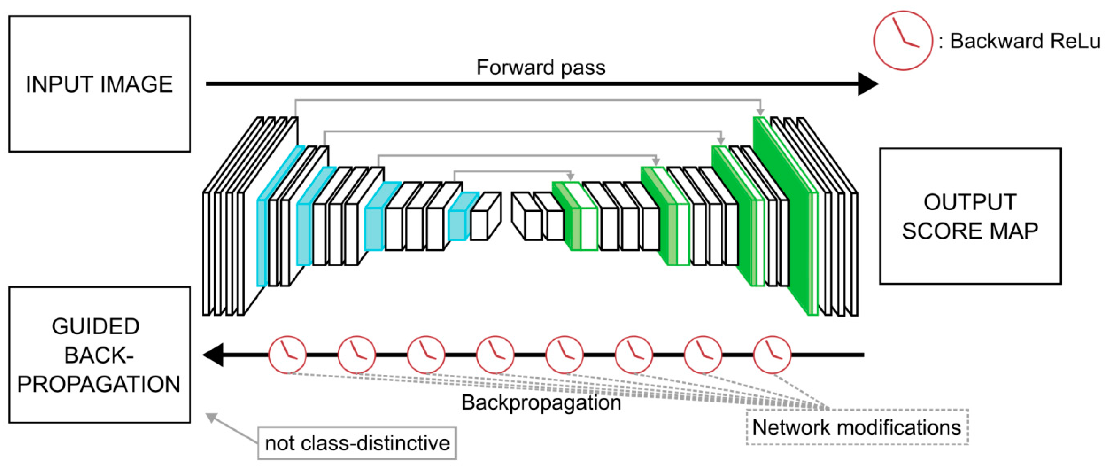
Relying on gradients can be problematic. CNNs are highly non-linear networks and some important features may have a large contribution globally but small effects on local scales. One approach to this is changing the network in such a way that only positive contributions pass during back-propagations, with all negative values being eliminated. One such strategy is guided back-propagation [5], which modifies the gradients of the rectified linear unit (ReLU) functions by discarding all negative values during the back-propagation calculation, thereby avoiding the problem. To adapt the guided back-propagation method to semantic segmentation, the back-propagation behavior of the model has to be modified. Given an input image, a forward pass to the last layer is performed, then all activations except one are set to zero and the gradient of the output map with respect to the input image computed. Figure 2 illustrates the computation of guided back-propagation in a sample segmentation network. As expected, the new map is much sharper and more detailed than the saliency map. Although guided back-propagation maps are easier to interpret, they are neither completely faithful to the model nor truly class distinctive [31]. An example is presented in Section 3.2.

2.8. Grad-CAM

The Grad-CAM [11] method is an improvement of CAM [10] and designed to address the shortcomings of CAM’s issues. It is possible to apply Grad-CAM to any convolutional neural network without any architectural modification where the networks’ final result map is differentiable with respect to its activation maps. As the output of a typical segmentation network is a 2D array, it is possible to use Grad-CAM to visualize features in the desired layer of a network. The method is highly class-distinctive and localizes different objects in a single input image. It produces regions with inherent smoothing and mapping from a lower resolution convolutional layer to the input layer produces maps that often correspond to intuition, since it is easier for humans to understand regions instead of discrete pixels [7]. The adapted method for semantic segmentation is shown in Figure 3. The selected layer to extract the Grad-CAM from is an additional hyper-parameter. In networks with an encoder-decoder architecture, selecting one of the last layers from the encoder network generates smoother maps. In an encoder-decoder architecture, dimensions of the middle layers’ feature maps (from the encoder network) are smallest among the network features. Upscaling (with interpolation) these small maps to match the input map generates smoother maps compared to the layers with larger dimensions, because much more upscaling is required. On the other hand, by selecting layers in the decoder part, the final map shows more detail and may highlight separated regions. This is because the generated map is computed using feature maps of the selected layer as well as the gradients of the output class with respect to the selected layer. Thus changing the layer generates different maps which are dependent on the selected layer. Maps generated with Grad-CAM can be considered as intermediate results for a segmentation network. Although this method is model-specific for CNNs and therefore not applicable to every network, it can help in understanding their internal functionality.

2.9. Guided Grad-CAM

Grad-CAM visualizations are class-discriminative and localize important regions in input images, but unlike gradient visualization methods they do not provide highly detailed pixel-space maps. Using pointwise multiplication combines the advantages of both guided back-propagation and Grad-CAM visualizations. The resulting guided Grad-CAM visualization is class-distinctive and of high resolution. The adaptation to semantic segmentation is shown in Figure 4. The process is similar to the original method [11], which aims to explain the decisions of classification networks. Based on guided Grad-CAM’s class-distinctness and high-resolution maps, it seems to be a superior visualization method. However, this assumption is only true if only interpretability, but not faithfulness is taken into account as well. Faithfulness is the ability to accurately explain the internal process of the model. Intuitively, there is a tradeoff between the interpretability and faithfulness: a more faithful visualization is typically less interpretable and vice versa [11]. The problem of measuring faithfulness and interpretability is that there is no actual ground truth for comparison. It is stated by [31] that Guided Grad-CAM is not faithful to a trained network and the results would be visually similar if the guided back-propagation map were replaced by an edge detection algorithm in the guided Grad-CAM method. It is a widely used visualization method nonetheless and can contribute to the understanding of a model.

2.10. Segmentation Score Maps

Segmentation score maps are a widely used means of evaluating a model’s performance. For segmentation networks, different measurements, like intersection over union (IoU) or pixel accuracy, exist. However, here we are interested in highlighting important pixels which contribute more to final predictions. A segmentation network generates a 2D score map for each class at the output layer as the result of the training process. The most commonly used loss function for this training is pixel-wise cross entropy loss and the target is the segmentation ground truth. Thus the ideal case is when these score maps are equal to the ground truth maps. It should be pointed out that there is an important difference between saliency and score maps. Saliency maps only take the pixels belonging to the chosen class into account, while score maps also consider pixels in the vicinity of the actual object pixels and the general context. True, it can be dependent on the architecture and use case: one example is context-aware architecture, but it also might occur in a biased model. Generally, not all features used in a network’s decision-making process are presented in the final layer because some of them might be removed. On the other hand, the network can be sensitive (for a class) to some features of the input image, but a different class wins the final pixel. In that case those passed over features might be interesting and worth studying.

2.11. Segmented Score Mapping

Score maps of the very last layer in a segmentation network can be interpreted as attributions of the model. They are information-rich and mappable to the input image. When compared to the final segmented map, score maps contain more information, but this information is not mapped to the segmented regions. One strategy is to merge information from different maps, for example score maps and segmentation maps. An example is segmented score mapping (SSM) based on the XRAI algorithm, introduced by [32]. XRAI identifies regions which are relevant to the predicted class by operating on the output of the integrated gradient. It targets semantic segmentation networks and uses score maps for attribution. To implement SSM, the so-called Felzenszwalb method is utilized [33]. It is governed by a set of hyper-parameters whose selection may affect the segmentation result. Performing the algorithm multiple times using different parameters is equivalent to over-segmenting. The final output result is a set of overlapping segmented regions. The SSM can be implemented in the following manner. First, the sum of attribution values for each area is computed to find the important regions. Subsequently the area with the maximum average value is added to an initially empty mask. The convergence criterion is reached when the mask size is equal to the input image.

2.12. Guided Segmented Score Mapping

A drawback of segmented score mapping is its independence upon the desired class. In order to remedy this, SSM can be augmented by additionally incorporating the final segmentation maps of all classes, resulting in the guided segmentation mapping (GSSM) method. The provided segmentation maps are over-segmented using an independent algorithm, Felzenszwalb for example, and all generated maps from the network output.

2.13. Similarity Mapping

A “similarity map” (SM) is a simplified version of a segmented score map (SSM) (see Section 3.2). It generates a visual representation for the similarity between classes in a semantic segmentation network by comparing a class attribution to output segmentation maps.

2.14. Fusion Score Mapping

Score maps are a result of the prediction process in a segmentation network. They are highly class-distinctive and provide scores for each pixel in each class. It is possible to examine them one by one—each time for a different class—which can be tedious for large numbers of classes, though. Combining all maps into a fusion score map can alleviate this problem by providing the combined information at a glance. A general approach to check outputs of segmentation networks is finding the maximum value for each pixel and then replacing it with the corresponding class, which is equivalent to the argmax function. The desired fusion score map can thus be generated by applying the max function without replacing corresponding classes. For a perfect segmentation model, the resulting fusion score map would be uniformly 1 for all pixels. In practice, however, model predictions are not without errors and thus different classes can be identified in the resulting map. Figuratively speaking, the fusion score map can be seen as a visualization of prediction probability.

2.15. Integration into Neuroscope

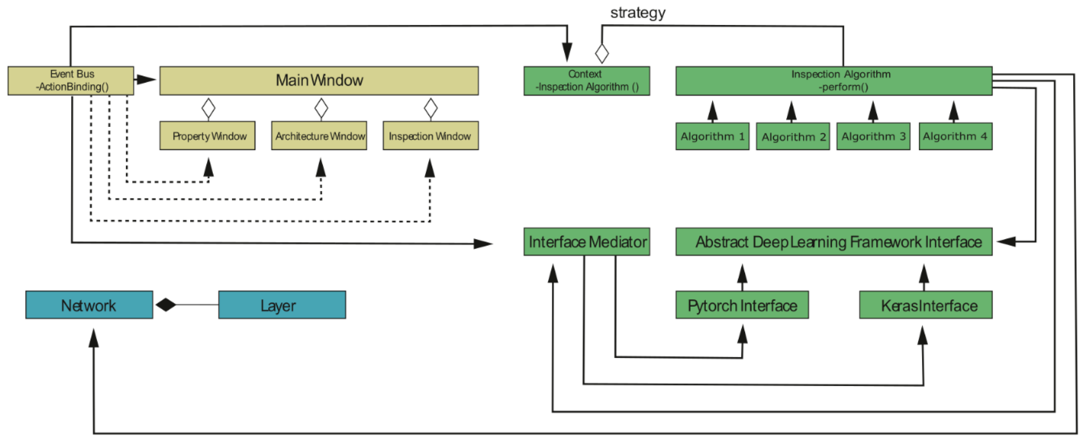
The graphical user interface of Neuroscope follows the model-view-controller (MVC) architecture design pattern [34], separating presentation and interaction from the system data, so that the system structure is divided into the three logical components model, view, and controller which interact with each other. Figure 5 shows the structure of Neuroscope in detail [35]. The classes in yellow in the diagram belong to the view component, including several windows and an event bus to bind the action in the window to the functionality implemented in the controller component. It is shown in green and is composed of two parts: strategy pattern and mediator pattern [34]. The strategy pattern includes the visualization algorithms presented in the previous chapter as well as several other algorithms. The mediator pattern contains the deep learning framework interfaces. The models themselves are handled by the model component rendered in blue.

3. Results

Section 3 explains the structure of Neuroscope and presents our adapted visualization methods for semantic segmentation. We demonstrate the functionality of Neuroscope using traffic images relevant to autonomous driving from the nuScenes data set [36]. It contains typical street situations with cars, pedestrians, and bicyclists from German, Swiss, and French cities.

3.1. Neuroscope Components

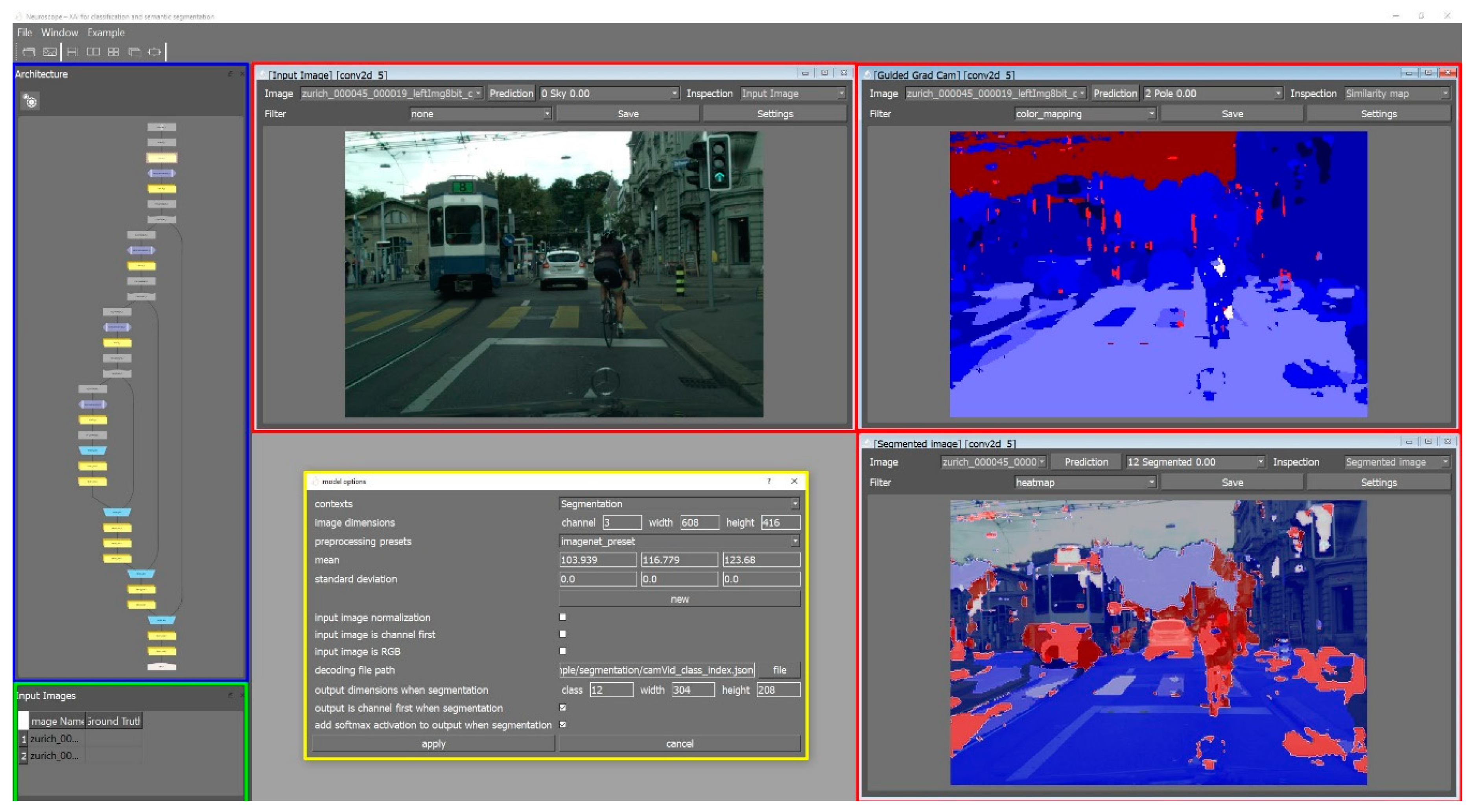
The Neuroscope graphical user interface (GUI) is composed of four main components: architecture view, model options, image list, and inspection windows, as shown in Figure 6.

3.1.1. Architecture View

A fundamental part of the Neuroscope GUI is the architecture window. It displays all layers of the chosen neural network and distinguishes between different layer types using both color coding and different shapes. This view allows layers of interest to be chosen for subsequent inspection. Following the layers from input to output in conjunction with suitable inspection views illustrates the development of a model’s internal behavior and thus helps the predictions to be better understood.

3.1.2. Model Options

Neural networks have many parameters required for an analysis of their behavior. The model options component queries the user to supply the relevant information about the model to be inspected. Parameters like input and output image dimensions and formats, preprocessing options, decoding files, and whether the model is intended for classification or segmentation, are set within this component.

3.1.3. Image List

The image list displays all images loaded for analysis by the user. For each of them, there may also be uploaded a corresponding ground truth image. This allows confusion matrices to be computed and the prediction to be evaluated according to a given metric, which can be chosen in the inspection window.

3.1.4. Inspection Window

The heart of Neuroscope is the inspection window. A selected image from the image list can be analyzed using a variety of visualization methods depending on the type of model—classification (C) or segmentation (S): input image (C,S), activation maps (C,S), saliency map (C,S), guided back-propagation (C,S), Grad-CAM (C,S), Guided Grad-CAM (C,S), Grad-CAM++ (C), score map (C,S), segmented score map SSM (S), guided segmented score map GSSM (S), similarity map (S), fusion score map FSM (S), confusion matrix (S, in conjunction with provided ground truth).

3.2. Application of Neuroscope to Real World Data

In this paper the focus is on presenting the novel semantic segmentation visualization capabilities of Neuroscope. The corresponding classification variants are implemented according to the state-of-the-art as detailed in the respective papers listed in Section 2, hence not demonstrated here explicitly.
As a state-of-the-art model for classification we employ VGG16 [37], while the semantic segmentation methods are illustrated using U-Net [2].

3.2.1. Comparing Different Visualization Methods

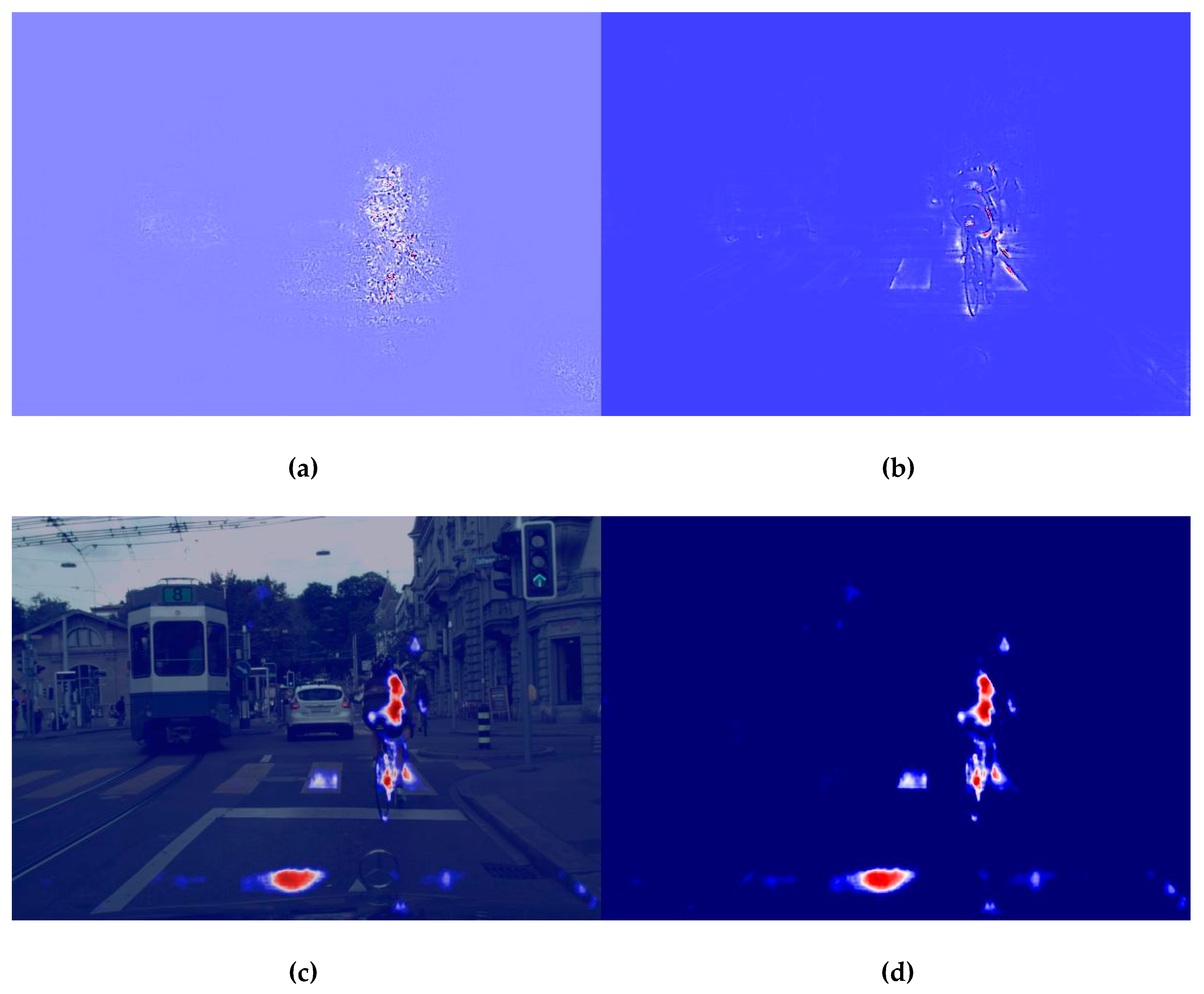
In Figure 7 different gradient-based visualization methods are compared for the class ‘bicyclist’. The saliency map (a) as the most basic algorithm shows a diffuse activation in the general vicinity of the bicyclist in the image but without sharp borders. Applying guided back-propagation (b) to the input image delivers a visually preferable result. The outlines of the bicyclist are clearly recognizable, as well as part of the pedestrian crossing’s stripes. The result of the Grad-CAM method (c) also highlights the bicyclist, but only the right-side part of the torso while ignoring the rest as well as the head. This is a consequence of the unpooling process during the decoding step of the U-Net–VGG16 network used for prediction. Compared to the previous two methods, a strong activation can also be observed in the lower middle of the image, where there is clearly no bicyclist located, but only a uniform patch of road. The same problem can be seen when using Guided Grad-CAM instead (d). Although the saliency map and guided back-propagation show the network is focusing on the correct part of the image, the result of the (Guided) Grad-CAM methods clearly indicates that there is an issue somewhere in the network, which should be addressed to further improve the prediction.
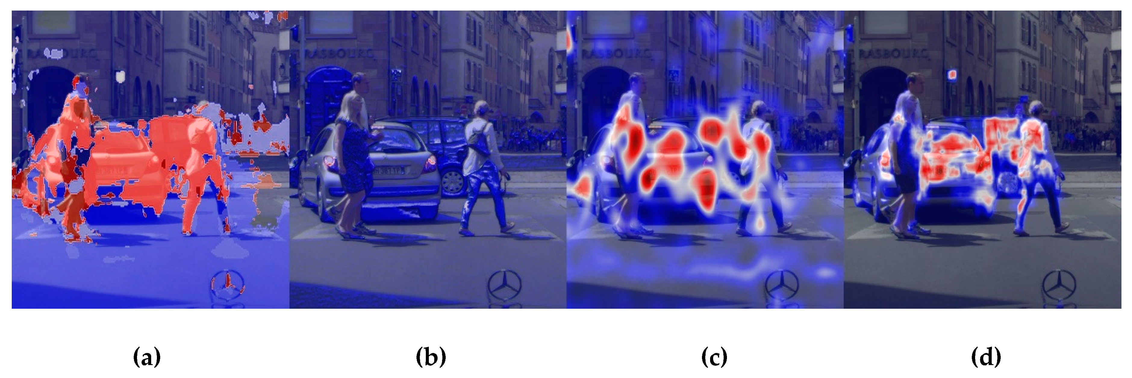
Figure 8 illustrates the behavior of a segmentation network when following the layers from input to output image. The Grad-CAM visualization for the class ‘car’ in an early layer (b) shows no distinct activation areas, the network at this stage is not predicting anything yet. The middle layer (c) on the other hand displays activity in the center of the image around the two cars, but includes both pedestrians as well. Inspecting the results of the final layer (d), the model has focused on both cars and excluded the left pedestrian while keeping the right one, compared to the middle layer. This visualization of a network’s evolution on different layers helps to understand how it arrives at its predictions. A conclusion drawn from the analysis with Neuroscope is that these two classes have shared features in this model. Thus adding more training images with cars and pedestrians, to increase the model’s distinction ability between these two classes could be a possible solution.

3.2.2. Guided Grad-CAM for Different Model Layers

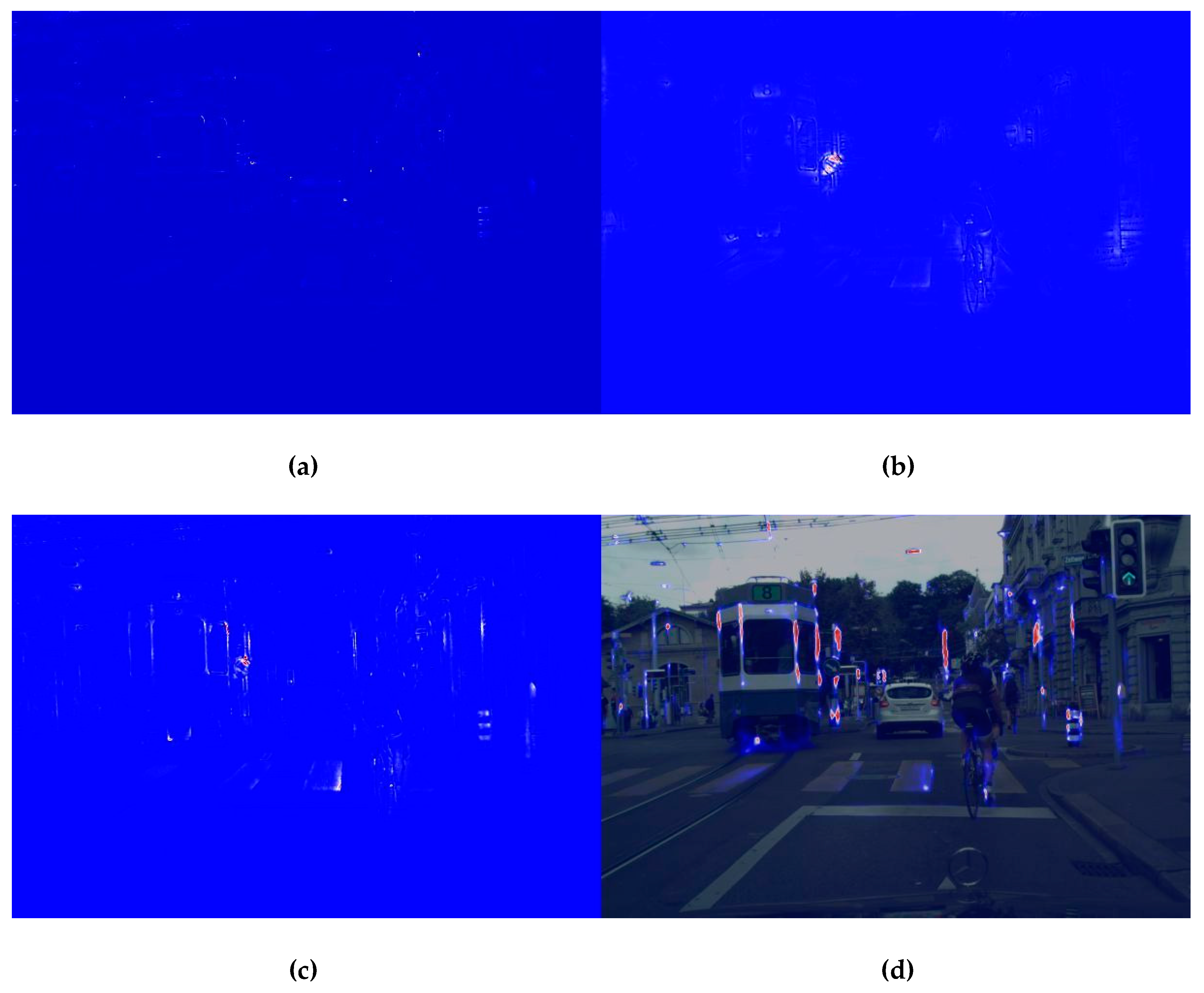
The visualization of the class pole with Guided Grad-CAM for various layers of a segmentation model is shown in Figure 9. Again, an evolution of the intermediate results can be seen by progressing from early through middle to final layers. In image (a) the network is not yet able to detect poles and shows a diffuse activation behavior. The middle layer (b) on the other hand focuses on a small patch of the tram and the bicyclist, both not pole-like structures. The final layer (c), however, exhibits several pole-like objects at first glance. Switching to a heat map view of the predicted segmentation (d), it can be seen that some of the poles predicted by the model are not poles at all, but part of the tram’s structure. Some poles in the middle and the right area of the image are correctly detected, but the right-hand side pole with the traffic lights is not recognized. The prediction thus contains both false negatives and false positives. The visualization with Neuroscope helps to detect the fact that the model starts heading in the wrong direction in the middle layer (b), where it focuses almost exclusively on the tram. Tweaking the layer topology in this part could remedy the problem.

3.2.3. Score Maps for Semantic Segmentation

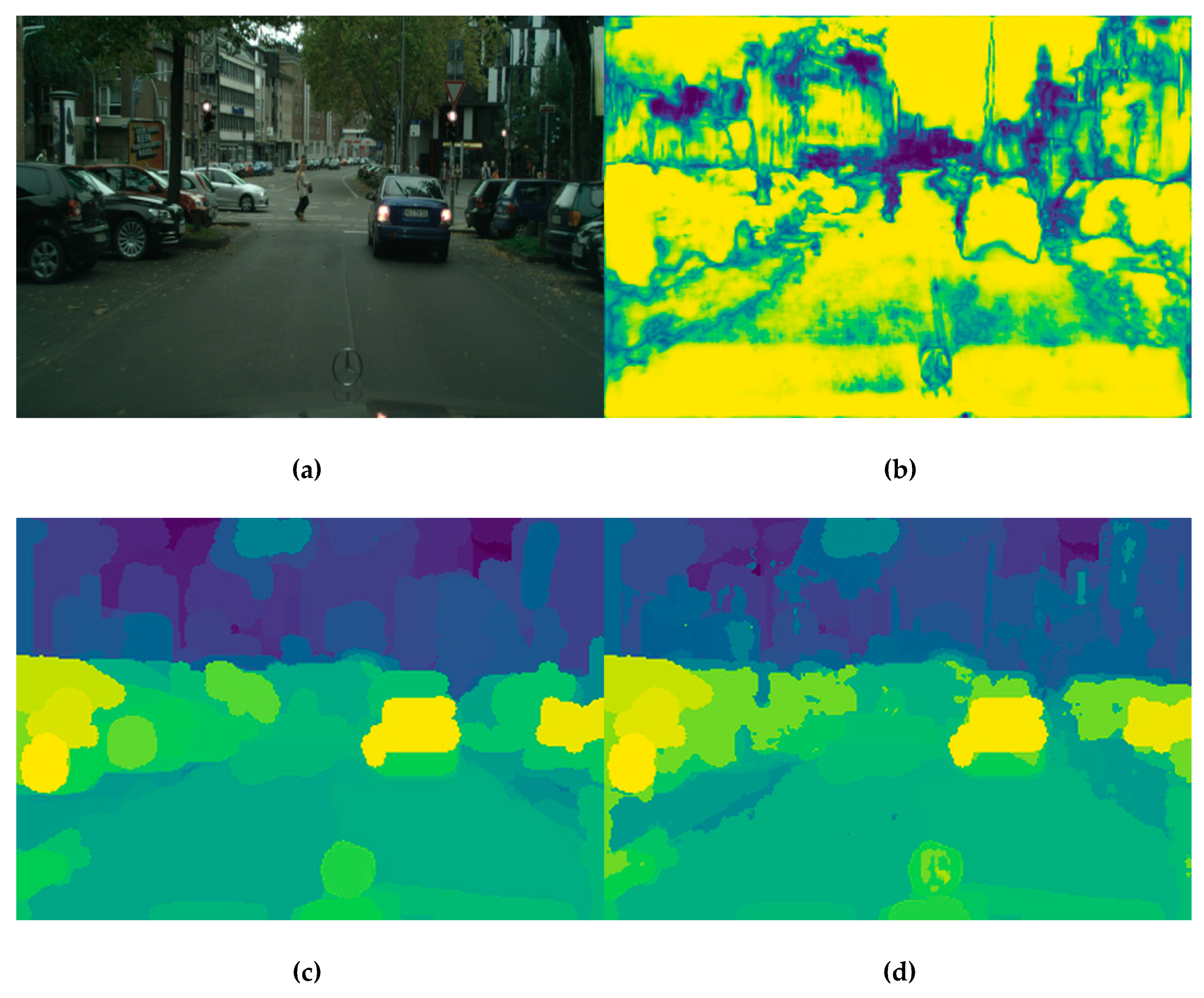
In Figure 10 the results of applying different segmentation score mappings on a traffic scene image for the class ‘car’ is shown. The fusion map (b) illustrates the scores of all classes simultaneously. The cars in the foreground of the image are highlighted in yellow while the smaller ones parking further along the street are rendered in dark blue, signaling their lower prediction probability. The pedestrian at the center of the image is shown in the same color and is thus also not reliably detected by the network. Compared to the basic segmentation score mapping (c) the guided version (d) shows finer details. Especially in the upper right corner of the image and to the left in the region of the parking cars. Note that the front wheel of the second car from the left is clearly recognizable in the SSM but not visible as a separate object in the GSSM visualization. Although the latter supplies a more detailed map, the former is more helpful in understanding the segmentation model.

4. Discussion

The field of explainable artificial intelligence is an evolving and highly debated one. Even the definition of ‘explanation’ in this context alone is not without controversy; for a comprehensive attempt to clarify the terminology refer to [38]. A general concern that has been raised in the scientific community is the question of whether post hoc methods are capable of really explaining black box-style deep neural networks or whether this approach is ultimately a dead end and research should be focused on inherently interpretable model designs. A comprehensive plea for this position is given in [39]. Especially for critical high stakes applications—like healthcare or recidivism prediction in the legal system—a fundamental understanding of the models may literally be a matter of life and death. A proposed solution is to design the models in such a way that they are inherently interpretable by humans and not only explainable in hindsight [40].
However, the vast majority of state-of-the-art models do not adhere to this design concept. At the moment it is much faster and cheaper for companies to implement deep neural networks using publicly available frameworks, like Tensorflow and out-of-the-box models like VGG16 or U-Net [2], rather than building interpretable models. Insight into the behavior of these already trained models may only be gained through post hoc methods like those provided by Neuroscope. The demand for such tools is obvious. Special care has to be taken in their application though. It must be kept in mind that it is difficult to distinguish errors of the model from errors of the attribution method explaining the model [7]. Thus, visualization-based evaluation tends to be qualitative in nature and partially biased by the humans performing it [41], caused by their preference for methods producing explanations matching their expectations over unexpected results. [31] has demonstrated that the widely used visualization method Guided Grad-CAM [11] delivers the same visual explanations when substituting the back-propagation step with an edge detection, so its explanations may not necessarily describe how the network really works. Therefore, it is critical to validate a preliminary explanation by additionally using different visualization methods and comparing the results to arrive at a conclusive explanation of the models’ behavior.

5. Conclusions

Neuroscope implements a wide range of visualization methods helping to understand how a neural network reaches its predictions. Exemplary application to real world traffic scenes from the nuScenes [36] data set shows that there is not one single visual explanation method which works best for all models and all input images. Different methods can be helpful in different situations, depending on their inherent advantages and disadvantages. For a meaningful and reliable explanation, multiple methods should be applied to the same data and their respective results fused into one comprehensive explanation. Neuroscope supports this task by allowing the analysis of a deep neural network step by step through all individual layers of its architecture.

Supplementary Materials

Neuroscope is available online at https://github.com/c3di/neuroscope (accessed on 3 March 2021), the nuScape data set can be downloaded at www.nuscenes.org (accessed on 3 March 2021).

Author Contributions

Conceptualization, F.C., P.G. and T.D.; software, F.C. and P.G.; writing—original draft preparation, C.S.; writing—review and editing, C.S.; visualization, C.S.; supervision, T.D. All authors have read and agreed to the published version of the manuscript.

Funding

This research was partly funded by European Commission, grant number 870130 in the course of the project COGNITWIN (Cognitive plants through proactive self-learning hybrid digital twins) in the program H2020. Parts of the research were also funded by the German Federal Ministry of Education and Research under grant number 19A19005G in the project KI-Absicherung.

Institutional Review Board Statement

Not applicable.

Informed Consent Statement

Not applicable.

Data Availability Statement

Data available in a publicly accessible repository, see Section 3.

Conflicts of Interest

The authors declare no conflict of interest.

References

  1. Gonzalez, R.C.; Woods, R.E. Digital Image Processing, 4th ed.; Pearson: New York City, NY, USA, 2018. [Google Scholar]
  2. Ronneberger, O.; Fischer, P.; Brox, T. U-Net: Convolutional Networks for Biomedical Image Segmentation. In Proceedings of the Medical Image Computing and Computer-Assisted Intervention—MICCAI 2015, Munich, Germany, 5–9 October 2015; Navab, N., Hornegger, J., Wells, W., Frangi, A., Eds.; Lecture Notes in Computer Science. Springer: Cham, Switzerland, 2015; Volume 9351, pp. 234–241. [Google Scholar] [CrossRef] [Green Version]
  3. Long, J.; Shelhamer, E.; Darrell, T. Fully convolutional networks for semantic segmentation. In Proceedings of the 2015 IEEE Conference on Computer Vision and Pattern Recognition (CVPR), Boston, MA, USA, 7–12 June 2015; pp. 3431–3440. [Google Scholar] [CrossRef] [Green Version]
  4. Zeiler, M.D.; Fergus, R. Visualizing and Understanding Convolutional Networks. In Proceedings of the Computer Vision–ECCV 2014, Zurich, Switzerland, 6–12 September 2014; Fleet, D., Pajdla, T., Schiele, B., Tuytelaars, T., Eds.; Lecture Notes in Computer Science. Springer: Cham, Switzerland, 2014; Volume 8689, pp. 818–833. [Google Scholar] [CrossRef] [Green Version]
  5. Springenberg, J.T.; Dosovitskiy, A.; Brox, T.; Riedmiller, M. Striving for Simplicity: The All Convolutional Net. In Proceedings of the Workshop Track Proceedings, 3rd International Conference on Learning Representations (ICLR), San Diego, CA, USA, 7–9 May 2015. [Google Scholar]
  6. Olah, C.; Satyanarayan, A.; Johnson, I.; Carter, S.; Schubert, L.; Ye, K.; Mordvintsev, A.R. The Building Blocks of Interpretability. Distill 2018, 3. [Google Scholar] [CrossRef]
  7. Sundararajan, M.; Taly, A.; Yan, Q. Axiomatic attribution for deep networks. In Proceedings of the 34th International Conference on Machine Learning Research (PMLR), Sydney, NSW, Australia, 6–11 August 2017; pp. 3319–3328. [Google Scholar]
  8. Bach, S.; Binder, A.; Montavon, G.; Klauschen, F.; Müller, K.-R.; Samek, W. On Pixel-Wise Explanations for Non-Linear Classifier Decisions by Layer-Wise Relevance Propagation. PLoS ONE 2015, 10. [Google Scholar] [CrossRef] [PubMed] [Green Version]
  9. Fong, R.; Vedaldi, A. Interpretable Explanations of Black Boxes by Meaningful Perturbation. In Proceedings of the IEEE International Conference on Computer Vision (ICCV), Venice, Italy, 22–29 October 2017; pp. 3429–3437. [Google Scholar] [CrossRef] [Green Version]
  10. Zhou, B.; Khosla, A.; Lapedriza, A.; Oliva, A.; Torralba, A. Learning Deep Features for Discriminative Localization. In Proceedings of the 2016 IEEE Conference on Computer Vision and Pattern Recognition (CVPR), Las Vegas, NV, USA, 27–30 June 2016; pp. 2921–2929. [Google Scholar] [CrossRef] [Green Version]
  11. Selvaraju, R.R.; Cogswell, M.; Das, A.; Vedantam, R.; Parikh, D.; Batra, D. Grad-CAM: Visual Explanations from Deep Networks via Gradient-Based Localization. In Proceedings of the 2017 IEEE International Conference on Computer Vision (ICCV), Venice, Italy, 22–29 October 2017; pp. 618–626. [Google Scholar] [CrossRef] [Green Version]
  12. Chattopadhay, A.; Sarkar, A.; Howlader, P.; Balasubramanian, V.N. Grad-CAM++: Generalized Gradient-Based Visual Explanations for Deep Convolutional Networks. In Proceedings of the 2018 IEEE Winter Conference on Applications of Computer Vision (WACV), Lake Tahoe, NV, USA, 12–15 March 2018; pp. 839–847. [Google Scholar] [CrossRef] [Green Version]
  13. Bau, D.; Zhou, B.; Khosla, A.; Oliva, A.; Torralba, A. Network Dissection: Quantifying Interpretability of Deep Visual Representations. In Proceedings of the 2017 IEEE Conference on Computer Vision and Pattern Recognition (CVPR), Honolulu, HI, USA, 21–26 July 2017; pp. 3319–3327. [Google Scholar] [CrossRef] [Green Version]
  14. Dhamdhere, K.; Sundararajan, M.; Yan, Q. How Important Is a Neuron? arXiv 2018, arXiv:1805.12233. [Google Scholar]
  15. Simonyan, K.; Vedaldi, A.; Zisserman, A. DeepInside Convolutional Networks: Visualising Image Classification Models and Saliency Maps. arXiv 2014, arXiv:1312.6034v2. [Google Scholar]
  16. Ribeiro, M.T.; Singh, S.; Guestrin, C. ‘Why Should I Trust You?’: Explaining the Predictions of Any Classifier. In Proceedings of the 22nd ACM SIGKDD International Conference on Knowledge Discovery and Data Mining, San Francisco, CA, USA, 13–17 August 2016; Association for Computing Machinery: New York, NY, USA, 2016; pp. 1135–1144. [Google Scholar] [CrossRef]
  17. Noh, H.; Hong, S.; Han, B. Learning Deconvolution Network for Semantic Segmentation. arXiv 2015, arXiv:1505.04366v1. [Google Scholar] [CrossRef] [Green Version]
  18. Mahendran, A.; Vedaldi, A. Visualizing Deep Convolutional Neural Networks Using Natural Pre-images. Int. J. Comput. Vis. 2016, 120, 233–255. [Google Scholar] [CrossRef] [Green Version]
  19. Chen, L.-C.; Papandreou, G.; Schroff, F.; Adam, H. Rethinking Atrous Convolution for Semantic Image Segmentation. arXiv 2017, arXiv:1706.05587. [Google Scholar]
  20. Tensorflow. Available online: https://wwwtensorflow.org (accessed on 11 December 2020).
  21. Tensorboard. Available online: https://www.tensorflow.org/tensorboard (accessed on 11 December 2020).
  22. Tensorflow Playground. Available online: https://playground.tensorflow.org (accessed on 11 December 2020).
  23. Wongsuphasawat, K.; Smilkov, D.; Wexler, J.; Wilson, J.; Mane, D.; Fritz, D.; Krishnan, D.; Viegas, F.; Wattenberg, M. Visualizing Dataflow Graphs of Deep Learning Models in TensorFlow. Trans. Vis. Comput. Graph. 2018, 24, 1–12. [Google Scholar] [CrossRef] [PubMed]
  24. Hohman, F.; Hodas, N.N.; Chau, D.H. ShapeShop: Towards Understanding Deep Learning Representations via Interactive Experimentation. Ext. Abstr. Hum. Factors. Comput. Syst. 2017. [Google Scholar] [CrossRef] [Green Version]
  25. Hohman, F.; Park, H.; Robinson, C.; Chau, D.H. SUMMIT: Scaling Deep Learning Interpretability by Visualizing Activation and Attribution Summarizations. Trans. Vis. Comput. Graph. 2019, 26, 1096–1106. [Google Scholar] [CrossRef] [PubMed] [Green Version]
  26. Wang, Z.J.; Turko, R.; Shaikh, O.; Park, H.; Das, N.; Hohman, F.; Kahng, M.; Chau, D.H. CNN EXPLAINER: Learning Convolutional Neural Networks with Interactive Visualization. Trans. Vis. Comput. Graph. 2020. [Google Scholar] [CrossRef]
  27. Park, H.; Hohman, F.; Chau, D.H. NeuralDivergence-Exploring and Understanding Neural Networks by Comparing Activation Distributions. arXiv 2019, arXiv:1906.00332v1. [Google Scholar]
  28. Kahng, M.; Andrews, P.; Kalro, A.; Chau, D.H. ActiVis: Visual Exploration of Industry-Scale Deep Neural Network Models. Trans. Vis. Comput. Graph. 2017, 24, 88–97. [Google Scholar] [CrossRef] [Green Version]
  29. Goodarzi, P. Visualizing and Understanding Convolutional Networks for Semantic Segmentation. Master’s Thesis, Saarland University, Saarbrücken, Germany, 2020. [Google Scholar]
  30. Vinogradova, K.; Dibrov, A.; Myers, G. Towards Interpretable Semantic Segmentation via Gradient-weighted Class Activation Mapping. In Proceedings of the Thirty-Fourth AAAI Conference on Artificial Intelligence, New York, NY, USA, 7–12 February 2020; AAAI Press: Palo Alto, CA, USA, 2020; pp. 13943–13944. [Google Scholar] [CrossRef]
  31. Adebayo, J.; Gilmer, J.; Muelly, M.; Goodfellow, I.; Hardt, M.; Kim, B. Sanity Checks for Saliency Maps. In Proceedings of the Advances in Neural Information Processing Systems 31, Annual Conference on Neural Information Processing Systems 2018 (NeurIPS), Montréal, QC, Canada, 3–8 December 2018; pp. 9505–9515. [Google Scholar]
  32. Kapishnikov, A.; Bolukbasi, T.; Viégas, F.; Terry, M. Segment Integrated Gradients: Better attributions through regions. CoRR 2019. [Google Scholar]
  33. Felzenszwalb, P.F.; Huttenlocher, D.P. Efficient Graph-Based Image Segmentation. Int. J. Comput. Vis. 2004, 59, 167–181. [Google Scholar] [CrossRef]
  34. Gamma, J.V.E.; Helm, R.; Johnson, R.E. Design Patterns. In Elements of Reusable Object-Oriented Software, 1st ed.; Addison-Wesley Publishing Company: Upper Saddle River, NJ, 1995. [Google Scholar]
  35. Chen, F. A Visual Explanation Tool on Multiple Deep Learning Frameworks for Classification Tasks. Master’s Thesis, Saarland University, Saarbrücken, Germany, 2019. [Google Scholar]
  36. Caesar, H.; Bankiti, V.; Lang, A.H.; Vora, S.; Liong, V.E.; Xu, Q.; Krishnan, A.; Pan, Y.; Baldan, G.; Beijbom, O. nuScenes: A multimodal dataset for autonomous driving. In Proceedings of the 2020 IEEE/CVF Conference on Computer Vision and Pattern Recognition (CVPR), Seattle, WA, USA, 14–19 June 2020; pp. 11618–11628. [Google Scholar] [CrossRef]
  37. Simonyan, K.; Zissermann, A. Very Deep Convolutional Networks for Large-Scale Image Recognition. arXiv 2014, arXiv:1409.1556v6. [Google Scholar]
  38. Roscher, R.; Bohn, B.; Duarte, M.F.; Garcke, J. Explainable Machine Learning for Scientific Insights and Discoveries. IEEE Access 2020. [Google Scholar] [CrossRef]
  39. Rudin, C. Stop Explaining Black Box Machine Learning Models for High Stakes Decisions and Use Interpretable Models Instead. Nat. Mach. Intell. 2019, 1, 206–2015. [Google Scholar] [CrossRef] [Green Version]
  40. Chen, C.; Lin, K.; Rudin, C.; Shaposhnik, Y.; Wang, S.; Wang, T. An Interpretable Model with Globally Consistent Explanations for Credit Risk. In Proceedings of the NeurIPS 2018 Workshop on Challenges and Opportunities for AI in Financial Services: The Impact of Fairness, Explainability, Accuracy, and Privacy, Montreal, QC, Canada, 3–8 December 2018. [Google Scholar]
  41. Ancona, M.; Ceolini, E.; Öztireli, C.; Gross, M. A unified view of gradient-based attribution methods for Deep Neural Networks. CoRR 2017. [Google Scholar]
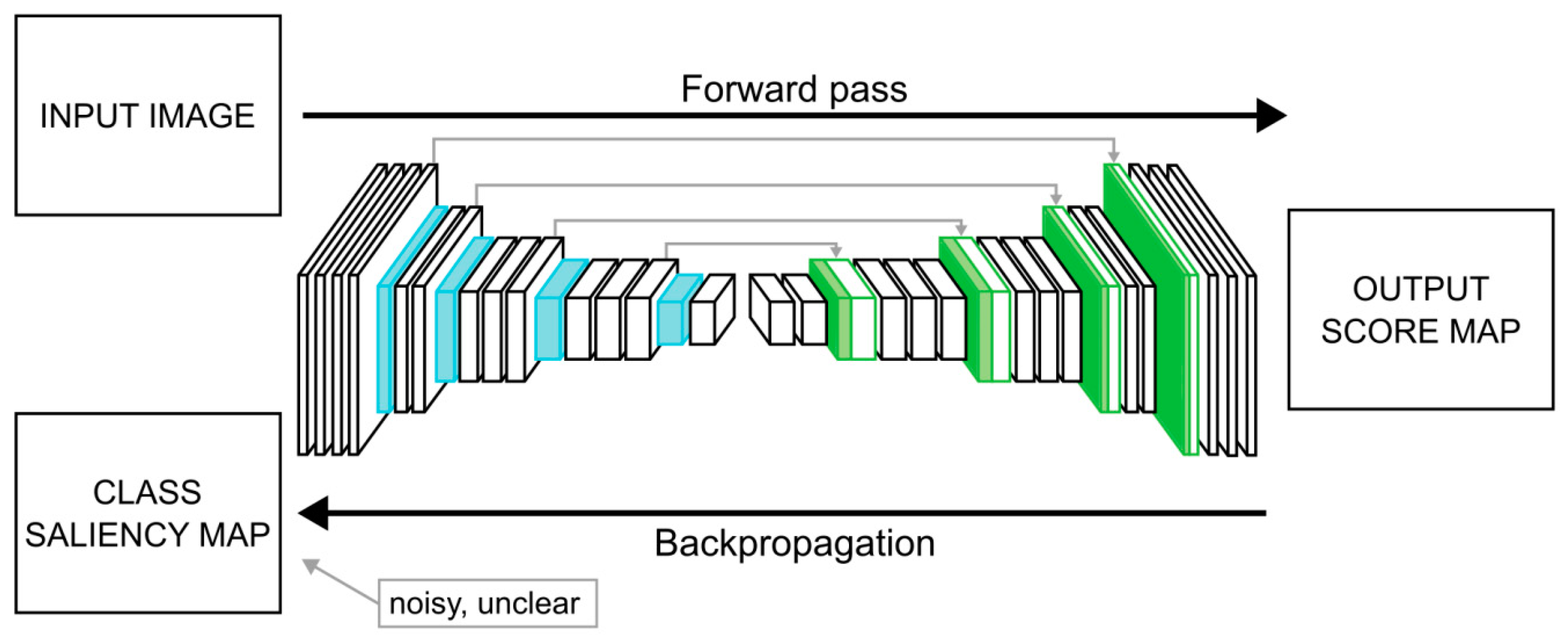
Figure 1. Class saliency map generation for semantic segmentation, computing the class saliency map of the output score map (class ‘car’) with respect to the input image. Brighter pixels indicate partial derivatives with higher absolute values.
Applsci 11 02199 g001
Figure 2. Applying guided back-propagation to a semantic segmentation network.
Applsci 11 02199 g002
Figure 3. Grad-CAM method for a segmentation network.
Applsci 11 02199 g003
Figure 4. Guided Grad-CAM for semantic segmentation.
Applsci 11 02199 g004
Figure 5. Schematic image of the structure of Neuroscope: model (model), view (yellow), controller (green).
Applsci 11 02199 g005
Figure 6. Screenshot of the Neuroscope graphical user interface (GUI): blue: architecture view, green: image list, yellow: model options, red: inspection windows.
Applsci 11 02199 g006
Figure 7. Different visualization methods for class ‘bicyclist’: (a) saliency map, (b) guided back-propagation, (c) Grad-CAM, (d) Guided Grad-CAM.3.2.2. Grad-CAM for Different Model Layers
Applsci 11 02199 g007
Figure 8. Grad-CAM visualizations for class ‘car’ on different layers of a model: (a) segmented image, (b) early layer, (c) middle layer, (d) final layer.
Applsci 11 02199 g008
Figure 9. Guided Grad-CAM visualizations for class ‘pole’ on different layers of a model: (a) early layer, (b) middle layer, (c) final layer, (d) segmented image.
Applsci 11 02199 g009
Figure 10. (a) Input image, (b) fusion score map (FSM), (c) segmented score mapping (SSM) for class ‘car’, (d) guided segmentation mapping (GSSM) for class ‘car’.
Applsci 11 02199 g010
Publisher’s Note: MDPI stays neutral with regard to jurisdictional claims in published maps and institutional affiliations.