Article

Hole Concealment Algorithm Using Camera Parameters in Stereo 360 Virtual Reality System

Department of Electrical Engineering, Sejong University, Seoul 05006, Korea
*
Author to whom correspondence should be addressed.
Appl. Sci. 2021, 11(5), 2033; https://doi.org/10.3390/app11052033
Submission received: 23 December 2020 / Revised: 15 February 2021 / Accepted: 22 February 2021 / Published: 25 February 2021
(This article belongs to the Section Electrical, Electronics and Communications Engineering)

1. Introduction

Virtual reality (VR) has been one of the most important topics in the field of multimedia signals and systems for approximately 10 years. There are many applications for 360 VR systems, such as broadcasting, movies, social media communication, remote education, and virtual tourism [1]. 360 VR images and videos are generated using a 360 VR camera rig or a spinning VR camera, which is usually expensive or consists of heavy equipment.
As the technologies related to VR have been studied, methods that use a general purpose camera or cheap smartphone instead of the technical equipment to generate a 360 VR image have been developed [2,3,4,5]. In [2], the authors explained a method to stitch images using direct alignment or feature-based alignment. When the feature-based alignment approach is employed, feature points are searched in each picture to be stitched using one of the related algorithms [6,7,8,9,10,11]. Then, the feature points are matched by RANSAC [12], which provides homography matrixes to represent the relationship between neighboring pictures with overlapping common regions. Intrinsic and extrinsic matrixes of each picture can be derived from the homography matrix. The intrinsic and extrinsic matrixes of all pictures to be used for generating a VR image are jointly optimized through a bundle adjustment procedure [13]. In [3], a real time algorithm was proposed to make a panoramic image from pictures taken by the camera of a mobile phone, where the resulting image is shown on a cylindrical surface. The pictures taken by a mobile phone have different colors and brightness values compared to other pictures because these depend on the direction and position of the camera used in taking the pictures. This difference produces various artifacts in the VR image. In order to reduce the degradation, an algorithm to find the seams and blend the overlapping regions was proposed in [4]. Automatic Panoramic Image Stitching (APIS) [5] is one of the most efficient methods to make the panorama image or VR pictures. APIS consists of a variety of modules explained in [2,7,8,11,12] which include the feature-based alignment, Scale Invariant Feature Transform (SIFT), Speed-Up Robust Features (SURF), Oriented FAST and Rotated BRIEF (ORB), Random Sample Consensus (RANSAC), bundle adjustment, straightening, and multiband blending.
In order to increase the quality of the stitched VR image, we can use high-end specialized equipment, for example GoPro VR cameras. When high-end specialized equipment is used to generate 360° VR images, it is considerably easier to align pictures without notable seam artifacts than that when using conventional cameras. Although VR images obtained from high-end specialized equipment have higher quality than those obtained from conventional cameras, conventional cameras are more affordable and simpler to use than specialized equipment. In fact, specialized equipment is bulky and expensive, thereby hindering its use in daily life.
With the increase in the viewer requirement for a sense of immersion, stereo 360 VR systems have been introduced to meet this need [14,15]. A stereo 360 VR image provides a more realistic and immersive sense to the viewer than a monocular 360 VR image, but the cost to make the contents increases further. The high cost of the equipment to generate 360 VR images may be one of the things preventing the spread of applications based on VR technology. This paper considers a system to generate a stereo 360 VR image using two cheap smartphones or two general purpose cameras attached to a rig.
In our scenario, because the general-purpose cameras are used to capture pictures, the pictures taken in arbitrary directions may produce non-overlapping regions and those become holes in the stitched image. In order to conceal the holes in stereo 360 VR images, various inpainting algorithms [16,17,18,19,20,21,22,23,24] can be considered as solutions, even though these were originally proposed for non-VR images. Bertalmio et al. [16] proposed an inpainting algorithm based on fluid dynamics, where a two-dimensional Navier–Stokes equation is approximated and combined with the Poisson equation for the vorticity. This approach produces an approximate solution for the holes in non-VR images. In the algorithm proposed by Telea et al. [17], each pixel in a hole is progressively concealed from the boundary to the center of the hole, where the value of a pixel to be concealed is set by the weighted average of the neighbouring pixels. Criminisi et al. [18] proposed a method to conceal a hole by filling it using a block. In this algorithm, the most similar patches are searched over a region around the hole. This scheme is a kind of template matching technique and the squared sum of the difference (SSD) is used as a criterion. On other hand, algorithms based on deep learning techniques were proposed in [19,20,21,22,23,24]. Liu et al. [19] proposed a deep learning-based method to conceal a hole in a non-VR image, where convolution weights are normalized by the mask area of the window. This effectively prevents the convolution filters from capturing too many zeros when they traverse over the incomplete region. When the deep learning-based algorithm is applied, the coefficients and variables in the convolutional network should be optimized for the huge quantity of training data. Thus, it requires a long training time and the performance depends on the type of training data. Note that certain conventional methods [16,17,18,19,20,21,22,23,24] use the data of the same camera stream to conceal the holes. In these techniques, the holes are filled based on the neighboring pixels and therefore their performances are limited when the size of the hole is large.
Unlike those techniques [16,17,18,19,20,21,22,23,24], when we fill the holes in the stereoscopic VR images, we use the data from the opposite camera stream. Using the data of the opposite camera stream is more efficient than using the data from the same camera stream, because the left and right views are correlated with each other. In order to compare the performances of two categories (using the data from same camera stream and opposite camera streams), we provide the simulation results obtained by methods in two categories in Section 4.
This paper proposes an efficient algorithm to conceal the holes in stereo 360 VR images, where camera parameters are utilized to estimate the location of the most similar fraction in other view images.
This paper is organized as follows. In Section 2, we formulate the problem, where two general purpose cameras are used to capture pictures for the left and right views. These pictures are used to generate stereo 360 VR images, where some blocks related to a hole are defined. In Section 3, we propose an efficient algorithm to conceal the holes, where the geometrical property of the pixels in VR images and the relationship between them are analyzed. Simulation results that demonstrate the performance of the proposed algorithm are provided in Section 4, where the performances of various techniques are compared subjectively and objectively. In Section 5, we provide a brief conclusion for this paper.

2. Problem Formulation

The Figure 1 shows the process used to make the stereo 360 VR images, which consist of left and right equi-rectangular projections (ERPs). In this configuration, the left and right cameras are mounted on a rig and capture pictures in the same direction, where general-purpose cameras (e.g., built-in cameras in smartphones) are used to capture pictures. The left and right ERPs are generated by applying several techniques to the sets of pictures with the left and right views. For example, the left ERP is made by consecutively applying feature extraction, mapping between features, a calculation of the homography matrix to represent the relationship, bundle adjustment to optimize the camera parameters, seam finding, and blending. The right ERP image is also made by a series of the same techniques. In this paper, APIS [5] is used to make the left and right ERPs, because it is known as one of the most efficient algorithms. APIS is applied independently to the left and right sets of pictures that have been captured by two built-in smartphone cameras. In this scenario, no mechanical equipment is used, other than a tripod. Thus, the pictures are captured in arbitrary directions and positions. Note that APIS does not include a function to conceal the holes in the stitched image. APIS is the basic style algorithm to stitch the pictures.
Figure 2 shows an example of the left and right ERPs that are generated using the procedure shown in Figure 1. As observed in Figure 2, we find some holes in these pictures. In the scenario illustrated in Figure 1, given that general-purpose cameras (instead of specialized equipment) are used, their narrow field-of-view (FOV) and the fact that pictures are often captured in arbitrary directions may produce non-overlapping regions and distortion (e.g., ghost effect or misalignment) in stitched 360° VR images. Non-overlapping regions also show up owing to the limitations of the stitching module, because the derivation of the relationship between spatially neighboring pictures is based on the RANSAC and feature points of each picture. The non-overlapping regions become holes in the stitched image, where the shape of the hole is dependent on the structure of the neighboring warped pictures. The shape of the holes may look like a square or a lozenge because those holes are surrounded by the neighboring warped pictures. Examples of the holes are shown in Section 4, where we can see the various shapes of holes.
In Figure 2, B L c is a block overlapping a hole in the left ERP. B L l and B L r are the left and right sides neighboring blocks of B L c , respectively. B R c , B R l , and B R r in the right ERP are blocks corresponding to B L c , B L l , and B L r , respectively. The corresponding blocks in the left and right ERPs are located in the same positions.
This paper proposes an efficient algorithm to conceal the holes, where pixels in the holes are filled with pixels in other ERPs and the location of the pixel used is derived from the camera parameters of the neighboring blocks { B R c , B R l , B R r , B L c , B L l , B L r }.

3. Algorithm Proposed to Conceal a Hole

3.1. Hole Detection

Figure 3 explains the process used to detect a hole in an ERP image. As observed in Figure 2, because a hole is a region that has not been covered by the warped pictures using the stitching algorithm, the color of the hole is black, with a luminance of zero. Thus, in step 1 of Figure 3, the colored ERP image is converted to a black-and-white picture to efficiently detect the holes. In step 2, all of the non-black pixels are replaced by white pixels, as shown in Figure 3c, where the black and white pixels have gray levels of 0 and 255 for an image represented with 8 bits/pixel, respectively. This results in the candidate regions for holes. Note that not all of the pixels in the dark objects have a zero value, even though some of the pixels in the objects may have a zero value. In order to classify the black pixels as hole and non-hole regions, a contour finding algorithm [25] is applied to image Figure 3c in step 3, which provides several contours with various sizes. In image Figure 3d, the perimeter of the contour of the hole is longer than that of a non-hole region, because the non-hole region is part of the dark object and it has the shape of an isolated particle. Therefore, if the length of the contour is shorter than a threshold, the dark region is removed, as shown in image Figure 3e. Finally, the block overlapping the dark region is set to B L c in image Figure 3e.

3.2. Camera Parameters of Neighboring Blocks

In Figure 1, when an ERP image is made, the stitching algorithm is applied to the set of pictures that have been taken by a single camera (the left or right camera). As explained in Section 2, each picture in a set of pictures with the left or right views is warped and translated according to the intrinsic matrix K and extrinsic matrix R of each picture. The following equations are the intrinsic and extrinsic matrixes of picture I i .
K ( I i ) = ( f x ( I i ) s ( I i ) c x ( I i ) 0 f y ( I i ) c y ( I i ) 0 0 1 )
R ( I i ) = ( r 11 ( I i ) r 12 ( I i ) r 13 ( I i ) r 21 ( I i ) r 22 ( I i ) r 23 ( I i ) r 31 ( I i ) r 32 ( I i ) r 33 ( I i ) )
where elements f x ( I i ) and f y ( I i ) are the horizontal and vertical focal lengths of the camera used, respectively. ( c x ( I i ) ,   c y ( I i ) ) is the location of the intersection between the Z axis of the world coordinate system and the plane of the image sensor. s is a skew coefficient. In (2), R is a rotation matrix used to represent the direction of camera lens when picture I i is taken. K and R are derived from a homography matrix calculated by RANSAC. The parameters in the K’s and R’s of all the pictures are optimized by the bundle adjustment based on the Levenberg–Marquardt algorithm [26].
As explained in Section 2, the blocks { B R c , B R l , B R r , B L c , B L l , B L r } have their own K’s and R’s, which can be represented by substituting { B R c , B R l , B R r , B L c , B L l , B L r } into I i in (1) and (2) as follows. As the equations have the same pattern, we represent those for B L l only.
K ( B L l ) = ( f x ( B L l ) s ( B L l ) c x ( B L l ) 0 f y ( B L l ) c y ( B L l ) 0 0 1 )
R ( B L l ) = ( r 11 ( B L l ) r 12 ( B L l ) r 13 ( B L l ) r 21 ( B L l ) r 22 ( B L l ) r 23 ( B L l ) r 31 ( B L l ) r 32 ( B L l ) r 33 ( B L l ) )

3.3. Concealment Based on Intrinsic and Extrinsic Matrixes

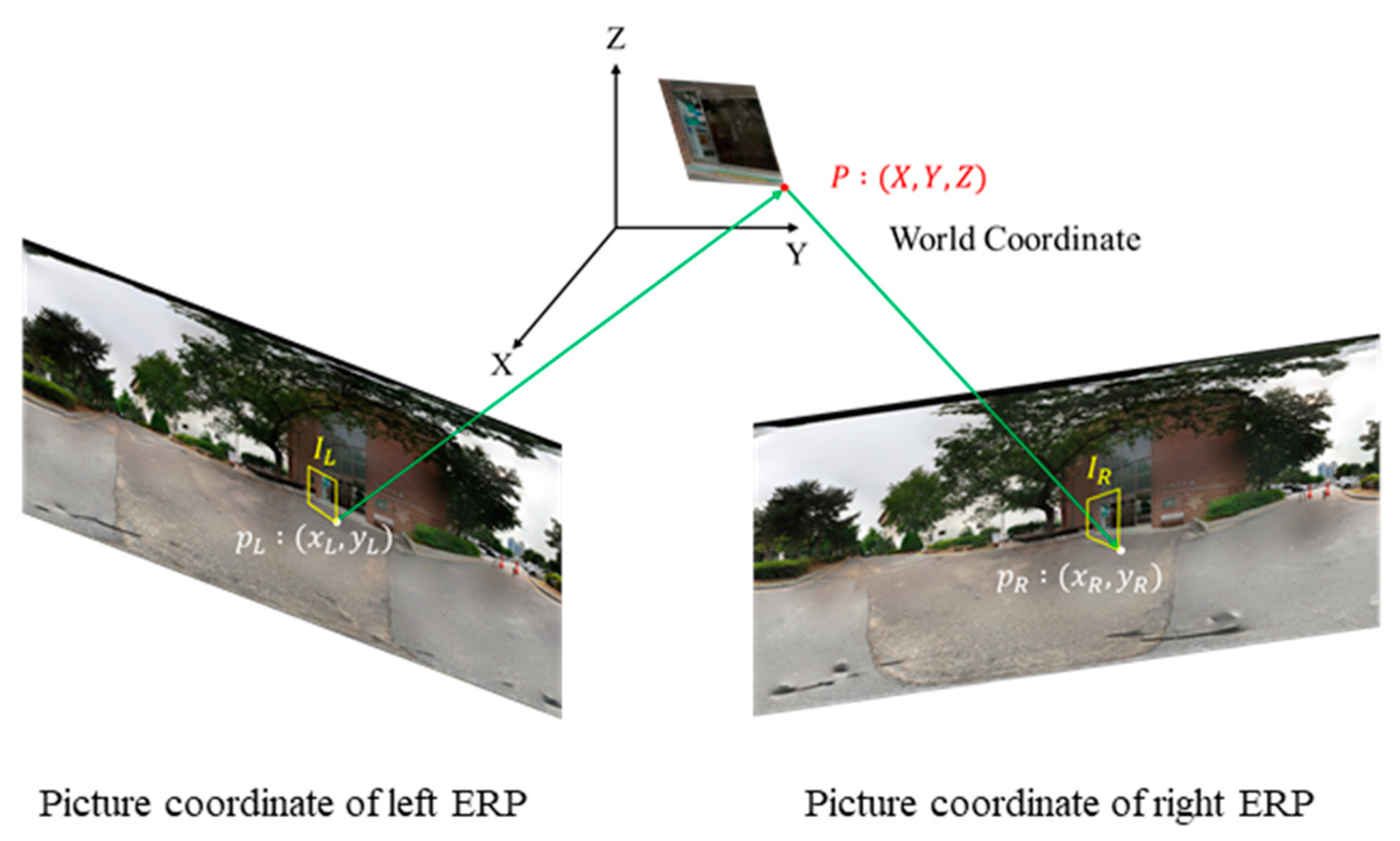
In this subsection, we derive the relationship between the stereo views, where the camera parameters of the warped pictures are utilized. In Figure 4, I L and I R are the warped images after they have been taken by the left and right cameras, respectively. Based on the geometric relation between the camera coordinate and world coordinate systems [27], the (X, Y, Z) of point P in the world coordinate system is mapped to the ( x L , y L ) and ( x R ,   y R ) of points p L and p R in I L and I R , respectively. The relation is represented as follows.
P = R ( I R ) K ( I R ) 1 p R
P = R ( I L ) K ( I L ) 1 p L  
Combining (5) and (6) gives
R ( I R ) K ( I R ) 1 p R = R ( I L ) K ( I L ) 1 p L
p R = K ( I R ) R ( I R ) 1 R ( I L ) K ( I L ) 1 p L
Therefore, the relation between the pixels in I L and I R can be represented with a 3 × 3 matrix H ( I L I R ) as follows.
p R = H ( I L I R ) p L
where
H ( I L I R ) = K ( I R ) R ( I R ) 1 R ( I L ) K ( I L ) 1  
The H ( I L I R ) can be calculated when K ( I R ) , R ( I R ) , R ( I L ) , and K ( I L ) are known. If I L and I R are replaced by B L c and B R c , respectively, then (10) becomes
H ( B L c B R c ) = K ( B R c ) R ( B R c ) 1 R ( B L c ) K ( B L c ) 1
In the proposed algorithm based on (11), each pixel in a hole is filled with a pixel in the right ERP, where H ( B L c B R c ) provides the location of the pixel in the right ERP to replace a particular pixel in a hole. This means that we can conceal the hole if K ( B R c ) , R ( B R c ) , R ( B L c ) , and K ( B L c ) are known.
On the other hand, when the hole is found in the right ERP, the following equation is used instead of (11).
H ( B L c B R c ) = K ( B L c ) R ( B L c ) 1 R ( B R c ) K ( B R c ) 1
Figure 5 shows an example of concealing each pixel in a hole when the hole is found in the left ERP.

3.4. Prediction for Camera Parameters

This subsection explains the method used to predict K ( B R c ) , R ( B R c ) , R ( B L c ) , and K ( B L c ) in order to derive H ( B L c B R c ) in (11). As shown in Figure 2, because B L c includes a hole, R ( B L c ) and K ( B L c ) are unknown. In addition, because B R c consists of fractions of multiple pictures in the right view, K ( B R c ) and R ( B R c ) should be recalculated instead of using those resulting from the process to make the right ERP. In order to predict { K ( B R c ) , R ( B R c ) , R ( B L c ) , K ( B L c ) } , the following operations are executed.
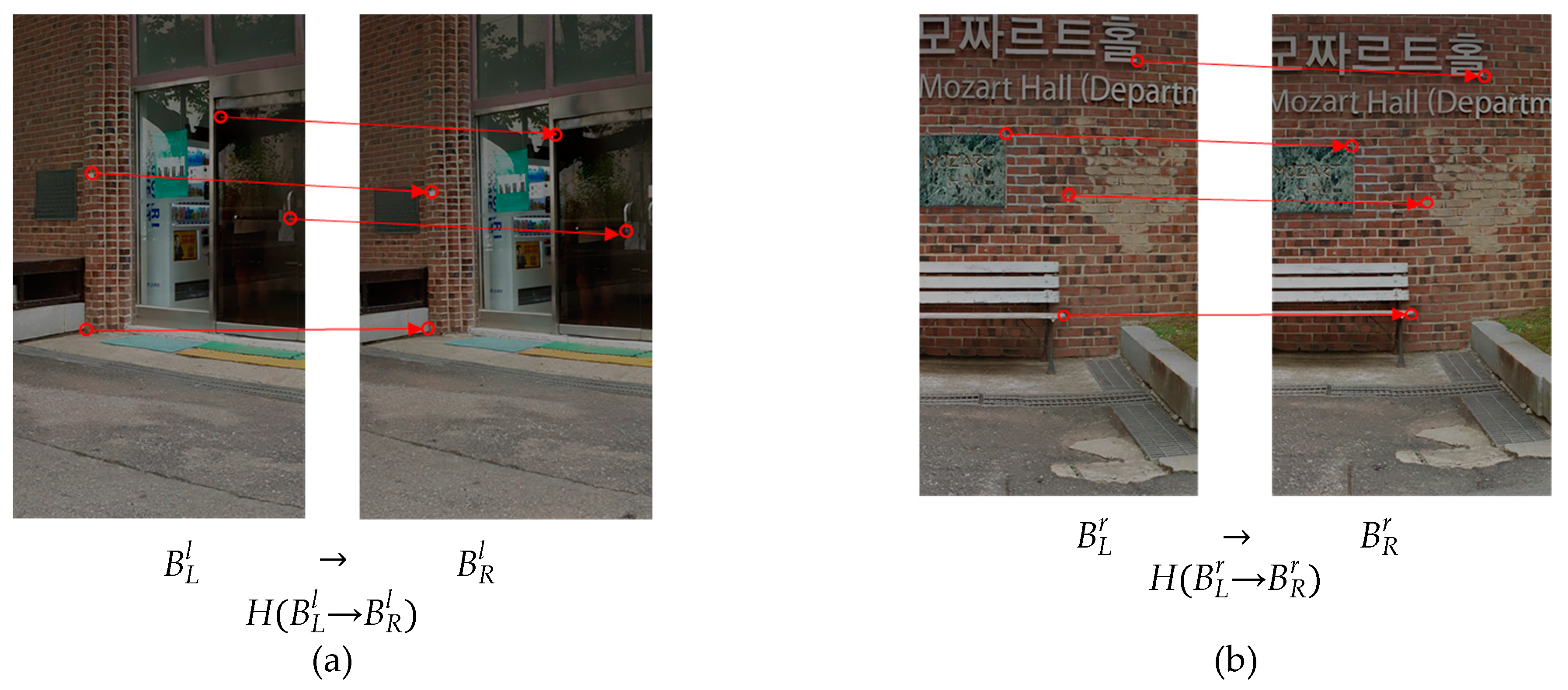
First, we estimate homography matrixes H ( B L l B R l ) and H ( B L r B R r ) for pairs { B L l , B R l } and { B L r , B R r }, respectively. H ( B L l B R l ) and H ( B L r B R r ) are derived by applying “feature extraction,” RANSAC, and “bundle adjustment” to those pairs. Figure 6 shows the examples used to estimate H ( B L l B R l ) and H ( B L r B R r ) , which have the following relationships.
H ( B L l B R l ) = K ( B R l ) R ( B R l ) 1 R ( B L l ) K ( B L l ) 1
H ( B L r B R r ) = K ( B R r ) R ( B R r ) 1 R ( B L r ) K ( B L r ) 1
From the homography matrixes in (13) and (14), { K ( B R l ) , R ( B R l ) , R ( B L l ) , K ( B L l ) } and { K ( B R r ) , R ( B R r ) , R ( B L r ) , K ( B L r ) } are derived by solving the simultaneous equations related to the focal length.
Second, R ( B R c ) and R ( B L c ) are estimated from { R ( B R l ) , R ( B L l ) } and { R ( B R r ) , R ( B L r ) }, respectively, which were obtained in the previous step. In [28], a rotation matrix R can be represented as a combination of rotational components R x , R y , R z on the x, y, z axes as follows.
R = R z ( θ ) R y ( σ ) R x ( ϕ ) = [ cos   θ sin   θ 0 sin   θ cos   θ 0 0 0 1 ] [ cos   σ 0 sin   σ 0 1 0 sin   σ 0 cos   σ ] [ 1 0 0 0 cos ϕ sin ϕ 0 sin ϕ cos ϕ ]
where ϕ , σ , and θ are the Euler angles about the x, y, and z axes, respectively. Applying the property to { R ( B L l ) ,   R ( B L c ) , R ( B L r ) , R ( B R l ) , R ( B R c ) , R ( B R r ) } gives
R ( B j i ) = R z ( θ ( B j i ) ) R y ( σ ( B j i ) ) R x ( ϕ ( B j i ) )
R x ( ϕ ( B j i ) ) = [ 1 0 0 0 cos ϕ ( B j i ) sin ϕ ( B j i ) 0 sin ϕ ( B j i ) cos ϕ ( B j i ) ]
R y ( σ ( B j i ) ) =   [ cos   σ ( B j i ) 0 sin   σ ( B j i ) 0 1 0 sin   σ ( B j i ) 0 cos   σ ( B j i ) ]
R z ( θ ( B j i ) ) =   [ cos   θ ( B j i ) sin   θ ( B j i ) 0 sin   θ ( B j i ) cos   θ ( B j i ) 0 0 0 1 ]
where i = {l, c, r} and j = {L, R}. In (16)–(19), ϕ ( B j i ) , σ ( B j i ) , and θ ( B j i ) are the Euler angles about the x, y, and z axes in R ( B j i ) , respectively. As observed in Figure 2, because B L c and B R c are located in the centers of { B L l and B L r } and { B R l and B R r }, respectively, we can assume that their Euler angles have the following relationships.
ϕ ( B j c ) = ϕ ( B j l ) + ϕ ( B j r ) 2  
σ ( B j c ) = σ ( B j l ) + σ ( B j r ) 2  
θ ( B j c ) = θ ( B j l ) + θ ( B j r ) 2    
where j = { L ,   R } . Substituting (20)–(22) into (16) provides R ( B L c ) and R ( B R c ) .
Third, K ( B L c ) and K ( B R c ) are estimated from { K ( B R l ) , K ( B L l ) } and { K ( B R r ) , K ( B L r ) }, respectively, which were derived in the first step. As we can see in (1), because the K matrixes consist of the focal length, aspect ratio, and center point, K ( B L c ) and K ( B R c ) can be derived by averaging the K’s of the neighboring blocks, as follows.
K ( B j c ) = K ( B j l ) + K ( B j r ) 2
where j = {L, R}.
Finally, because we obtained { K ( B R c ) , R ( B R c ) , R ( B L c ) , K ( B L c ) } in the previous steps, substituting them into (11) results in H ( B L c B R c ) , which can be used to conceal each pixel in a hole.

3.5. Summary of the Proposed Algorithm

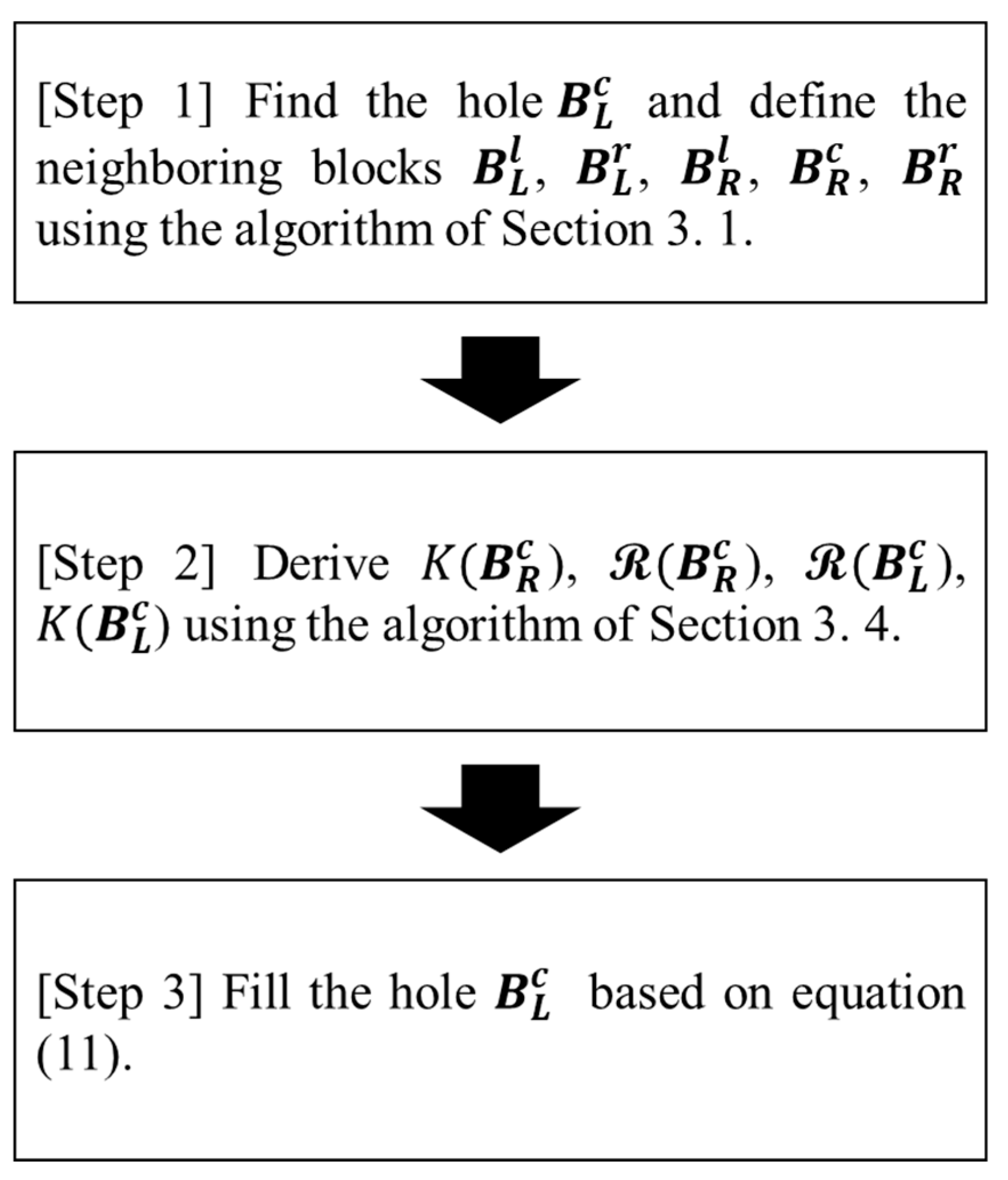
Figure 7 summarizes the proposed algorithm. In the first step, the hole is found using the algorithm described in Section 3.1, where the hole B L c and the neighboring blocks B L l , B L r , B R c , B R l , and B R r are defined according to the relationship between their coordinates. In the second step, we derive K ( B R c ) , R ( B R c ) , R ( B L c ) , and K ( B L c ) using the algorithm proposed in Section 3.4. In the third step, each pixel in the hole B L c is filled with the corresponding pixel in the right ERP, where the H ( B L c B R c ) of (11) provides the coordinate of the corresponding pixel. When the hole is in the right VR image, H ( B L c B R c ) of (12) is used to fill the hole.
The main characteristics of the proposed algorithm are as follows: First, the proposed algorithm conceals the holes in stereoscopic VR images, whereas most conventional algorithms [16,17,18,19,20,21,22,23,24,29] for filling holes were proposed for non-VR images. In particular, certain concealment algorithms [30,31,32] were proposed to fill the holes in depth images, where the holes have arbitrary shapes and some of them are small particles. Second, our algorithm can derive the location of the most similar pixel for each pixel in a hole. In our scenario, we use the data of the camera stream of another view to fill the holes, where the exact location of the most similar part should be calculated to increase the objective and subjective quality of the filled region. The position is estimated by analyzing Euler angles of extrinsic matrices of the related neighbor blocks. In the analysis of Euler angles, we decompose the angles along x, y, and z axes and then merge them to find the exact location of the reference data. The relevant explanation is provided in Section 3.4.

4. Simulation Results

In order to demonstrate the performance of the proposed algorithm, we compare it with various conventional methods, including those of Bertalmio [16], Telea [17], Criminisi [18], Liu [19], GiliSoft Stamp Remover [33], and Theinpaint [34] from the subjective and objective viewpoints. These methods were explained in Section 1.
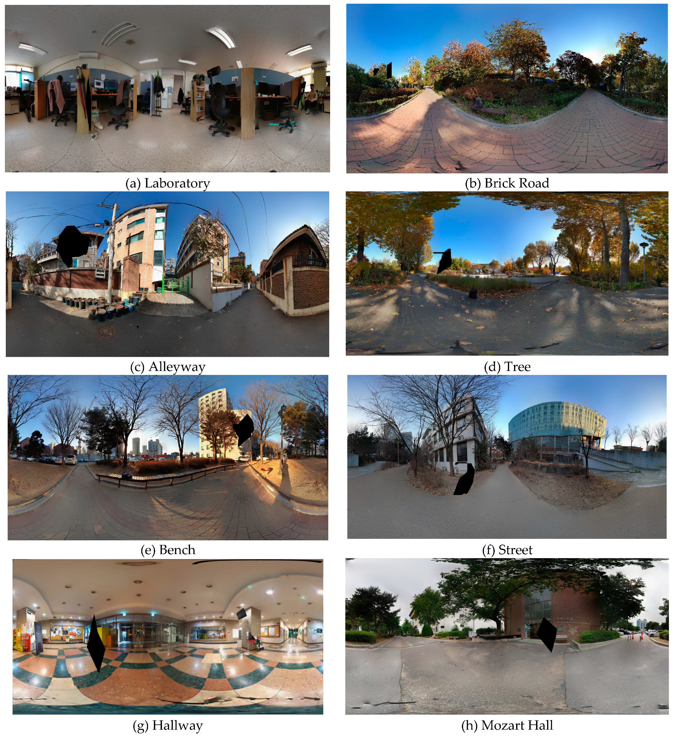
We captured picture sets using the built-in camera of a Samsung Galaxy 9 smartphone. There were more than 100 pictures in each set. The pictures within a single set were stitched using APIS to create the stereoscopic VR images. Figure 8 shows the left or right VR images of the stereoscopic VR images having holes of various sizes and locations. The VR images including the holes were used as test sets to evaluate the performances of the proposed algorithm and various conventional methods. In Figure 8a–f, the holes have been generated through the stitching algorithm owing to the reason described in Section 2. Those pictures are used only for subjective evaluations because there is no reference VR image without any hole. When we created Figure 8g,h, the stitched VR images did not have any holes. Therefore, we have made an artificial hole in each VR image. Consequently, Figure 8g,h can be used for objective evaluation, because the difference between the reference image (without any hole) and the concealed images (the results of various algorithms) can be calculated numerically.

4.1. Subjective Performance

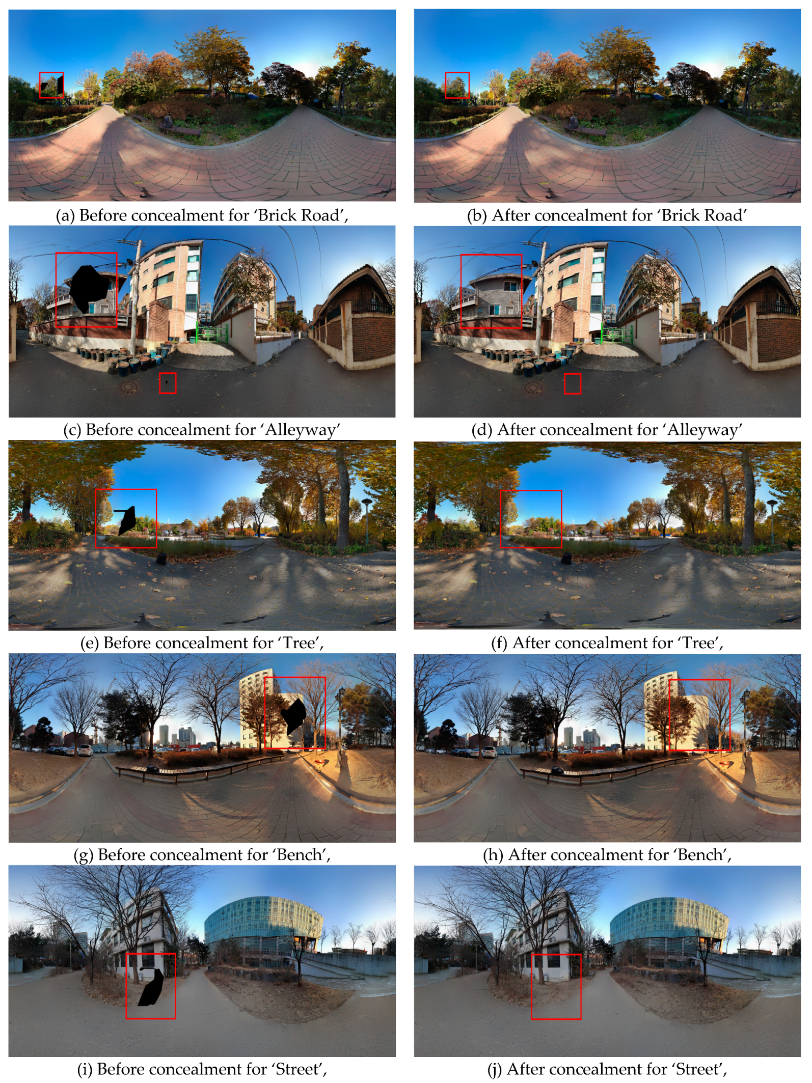
In order to check the performance of the proposed algorithm, we applied the proposed algorithm for the test sets of Brick Road, Alleyway, Tree, Bench, and Street. In Figure 9, VR images including the holes are compared with the concealed images, respectively. As shown in Figure 9, we can see that the proposed algorithm conceals the various holes effectively in the test images.
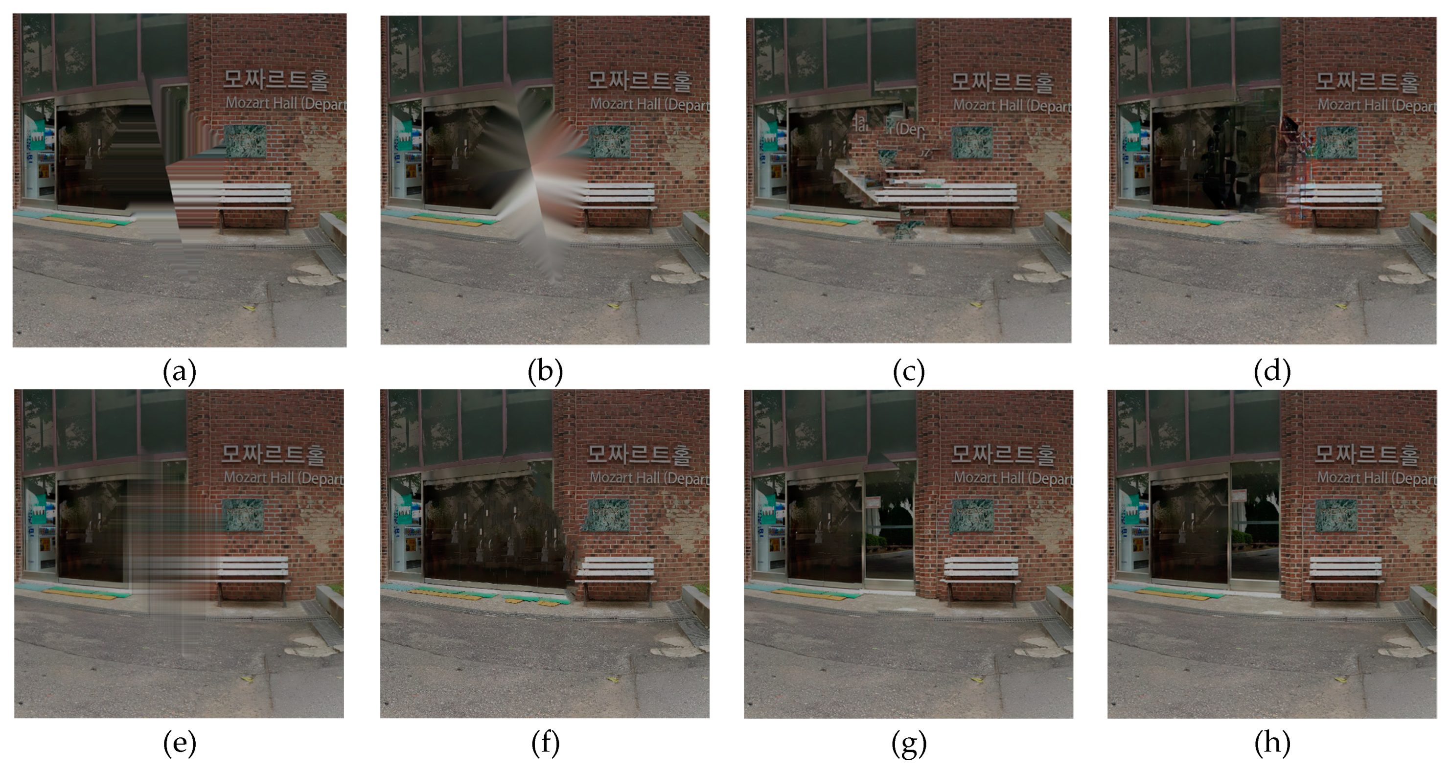
To compare the performances of various techniques subjectively, the pictures whose holes have been concealed by the methods are shown in Figure 11, where all of the pictures are a part of the left ERP picture and we made a hole artificially as Figure 10b in order to compare the concealed pictures Figure 11a–h with the reference image Figure 10a.
As observed in Figure 11, the proposed algorithm outperforms the other techniques subjectively. In the picture Figure 11a result from Bertalmio [16], the pixels in the hole are filled by copying the neighboring pixels horizontally or vertically. Thus, the concealed region has artifact lines. When the method of Telea [17] is used to conceal the hole, each pixel in a hole is concealed progressively from the boundary to the center of the hole, where the value of the concealed pixel is set to the weighted sum of the values of the neighboring pixels. Thus, the concealed region of Figure 11b has smoothed and diffused distortion. In Figure 11c, when the method of Criminisi [18] is used, the pixels in the hole are filled by blocks, where the template matching algorithm is used. In this method, the SSD of template part is considered a cost function to estimate the most similar block, and the values of the pixels in the non-template part are not considered. Thus, some pixels in the hole are filled with wrong values. As shown in Figure 11d, the method of Liu [19] based on deep learning has filled the hole with inappropriate blocks, which are generated from the deep learning engine. Figure 11e,f were resulted from Gilisoft stamp remover [33] and Theipaint [34], respectively. As shown in Figure 11e,f, these methods does not remove the holes completely. In Figure 11g, the hole in the left ERP is concealed just by copying a block in the right ERP, where the shapes and coordinates of the blocks, including the hole in the left ERP and the copied block in the right ERP, are same. As observed in Figure 11g, the concealed region has significant mismatches around the hole, because this method does not consider the disparity between the left and right views. Whereas the conventional techniques have serious artifacts in the concealed region, the image Figure 11h produced by the proposed algorithm has a natural and continuous boundary in the concealed region.
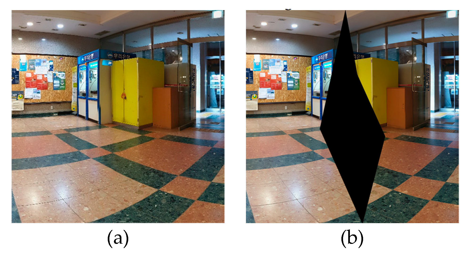
Figure 12 and Figure 13 show the simulation results for indoor pictures, where the size of the hole is bigger than that of Figure 10 and Figure 11. As can be seen from Figure 12 and Figure 13 and Figure 10 and Figure 11, the performance tendencies of the various algorithms do not change even if the size of the hole is varied.
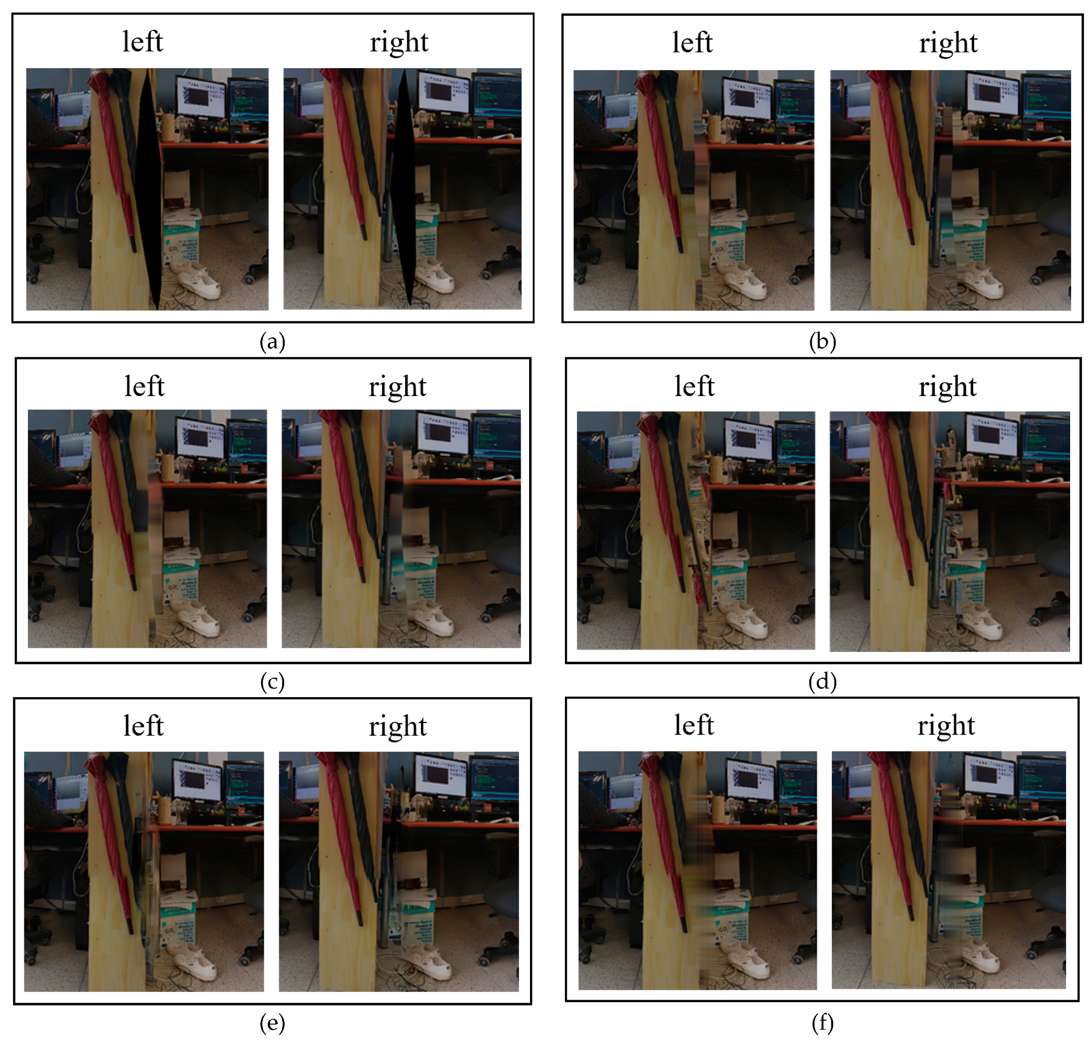
Figure 14 shows the simulation results for the naturally generated holes that occurred non-artificially during the stitching procedure. Note that no reference picture was used in this test. In this configuration, both the left and right ERP images had holes at different locations independently. In this test, the concealment algorithms were applied to the left and right ERP pictures independently. The results of the conventional and proposed techniques are shown in Figure 14b–g,h, respectively. When the proposed algorithm was applied, Equations (11) and (12) were used to conceal the holes in the left and right ERPs, respectively. As observed in Figure 14, the proposed method outperformed the other conventional techniques subjectively. In addition, the performance tendencies of the techniques were the same as those of Figure 10 and Figure 11 and Figure 12 and Figure 13.

4.2. Objective Performance

The objective performances of the concealment algorithms were evaluated with common measures like the structural similarity (SSIM) [35], peak-to-peak signal-to-noise ratio (PSNR) [36], and consumed CPU time. All experiments are run on the CPU based on AMD Ryzen 3.40 GHz and 32-GB RAM. The SSIM and PSNR are the average values of the SSIM and PSNR values for the red, green, and blue components. SSIM is in the range of 0–1. As the values of SSIM and PSNR increase, the quality of the resulting image increases. Note that SSIM and PSNR can be evaluated when the reference pictures are given, as in Figure 10 and Figure 11 and Figure 12 and Figure 13.
On the other hand, the CPU times consumed by the methods were checked using a personal computer. The CPU time was measured with the resolution of a second. As the CPU time depended on the complexity of the algorithm, the technique consuming the smallest CPU time was considered the simplest method.
The outdoor pictures (Mozart Hall) shown in Figure 10 and Figure 11 are evaluated in Table 1 and Table 2, where the best and 2nd best results are represented with red and blue numbers, respectively. As seen in Table 1, the proposed algorithm produced the best quality from the viewpoints of both the SSIM and PSNR. Theipaint [34] had the 2nd best quality for both SSIM and PSNR. The “simple copy” required the smallest CPU time, because it filled the hole just by copying the same size block of the other view. The proposed algorithm is one of the simplest algorithms in the consumed time. When the method of Liu [19] was used, the consumed CPU time could not be measured because the training time was huge and depended on the quantity of the training data.
Table 2 shows the performances of the proposed algorithm for a variety of sizes of neighboring blocks { B R l ,   B R r , B L l , B L r }, where the numbers in the first column denote the ratio between the widths of neighboring block B L l and block B L c that includes the hole. As observed in this table, the best performance is found when the ratio is 1.5 (i.e., the width of B L l is 50% wider than that of B L c ).
When the size of the neighboring blocks is small (the ratio is under 1.5), the performance of the proposed algorithm increases with the size, because the accuracy of H ( B L c B R c ) increases as the number of pixels utilized to derive it increases. However, when the size is large (the ratio is over 1.5), the neighboring blocks include fractions of multiple pictures, which degrades the accuracy of H ( B L c B R c ) . In this table, the complexity increases with the width of the neighboring blocks, because the number of pixels to be considered in making H ( B L l B R l ) and H ( B L r B R r ) increases.
Table 3 and Table 4 show the simulation results for the indoor pictures (Hallway) shown in Figure 12 and Figure 13. Note that the hole in Figure 12 and Figure 13 are larger than that of Figure 10 and Figure 11. As observed in Table 3 and Table 4, the performance tendencies of the methods are similar to those seen in Table 1 and Table 2. As observed in Table 3, the proposed algorithm has the best performance. Gilisoft [33] and Theipaint [34] had the 2nd best quality for PSNR and SSIM, respectively. The 2nd best performance is seen for the different ratios in Table 2 and Table 4 because the pictures of Figure 12 and Figure 13 include more complex regions and larger holes than those of Figure 10 and Figure 11.
From the results in Table 1, Table 2, Table 3 and Table 4, we can see that the proposed algorithm outperforms the conventional methods objectively.

5. Conclusions

We proposed an efficient algorithm to conceal the holes generated in stereo VR pictures, where the positions of the pixels to fill the hole were derived using the camera parameters. The camera parameters were predicted from their relationship with the homography matrix. Whereas conventional inpainting algorithms have constraints in the concealment of the hole because they were invented for non-VR images, the proposed method efficiently fills all of the pixels in the hole using the relationship between the left and right ERPs.

Author Contributions

Conceptualization, J.-K. H.; Data curation, S. C. and D.-Y. N.; Formal analysis, S. C., D.-Y. N. and J.-K. H.; Funding acquisition, J.-K. H.; Investigation, S. C. and J.-K. H.; Methodology, S. C. and J.-K. H.; Resources, J.-K. H.; Software, S. C.; Supervision, J.-K. H.; Visualization, J.-K. H.; Writing—original draft, S. C.; Writing—review & editing, J.-K. H. All authors have read and agreed to the published version of the manuscript.

Funding

This work was partially supported by the National Research Foundation of Korea (NRF) under Grant NRF-2018R1A2A2A05023117 and partially by the Institute for Information & Communications Technology Promotion (IITP) under Grant 2017-0-00486 funded by the Korea government (MSIT).

Institutional Review Board Statement

Not applicable.

Informed Consent Statement

Not applicable.

Data Availability Statement

The data presented in this study are available on request from the corresponding author.

Conflicts of Interest

The authors declare no conflict of interest.

References

  1. Zhang, K.; Liu, S.J. The application of virtual reality technology in physical education teaching and training. In Proceedings of the 2016 IEEE International Conference on Service Operations and Logistics, and Informatics (SOLI), Beijing, China, 10–12 July 2016; pp. 245–248. [Google Scholar]
  2. Szeliski, R. Image Alignment and Stitching: A Tutorial, Foundations and Trends in Computer Graphics and Computer Vision; Now Publishers: Delft, The Netherlands, 2006; Volume 2, p. 120. [Google Scholar]
  3. Kim, B.S.; Lee, S.H.; Cho, N.I. Real-time panorama canvas of natural images. IEEE Trans. Consum. Electron. 2011, 57, 1961–1968. [Google Scholar] [CrossRef]
  4. Xiong, Y.; Pulli, K. Fast panorama stitching for high-quality panoramic images on mobile phones. IEEE Trans. Consum. Electron. 2010, 56, 298–306. [Google Scholar] [CrossRef] [Green Version]
  5. Brown, M.; Lowe, D.G. Automatic panoramic image stitching using invariant features. Int. J. Comput. Vis. 2007, 74, 59–73. [Google Scholar] [CrossRef] [Green Version]
  6. Viswanathan, D.G. Features from accelerated segment test (fast). In Proceedings of the 10th Workshop on Image Analysis for Multimedia Interactive Services, London, UK, 6–8 May 2009; pp. 6–8. [Google Scholar]
  7. Lowe, D.G. Distinctive image features from scale-invariant keypoints. Int. J. Comput. Vis. 2004, 60, 91–110. [Google Scholar] [CrossRef]
  8. Bay, H.; Tuytelaars, T.; Van Gool, L. Surf: Speeded up robust features. In European Conference on Computer Vision; Springer: Berlin/Heidelberg, Germany, 2006; pp. 404–417. [Google Scholar]
  9. Calonder, M. Brief: Binary robust independent elementary features. In European Conference on Computer Vision; Springer: Berlin/Heidelberg, Germany, 2010; pp. 778–792. [Google Scholar]
  10. Leutenegger, S.; Chli, M.; Siegwart, R.Y. BRISK: Binary robust invariant scalable keypoints. In Proceedings of the 2011 International Conference on Computer Vision, Barcelona, Spain, 6–13 November 2011; pp. 2548–2555. [Google Scholar]
  11. Rublee, E. ORB: An efficient alternative to SIFT or SURF. In Proceedings of the 2011 International Conference on Computer Vision, Barcelona, Spain, 6–13 November 2011; pp. 2564–2571. [Google Scholar]
  12. Fischler, M.A.; Bolles, R.C. Random sample consensus: A paradigm for model fitting with applications to image analysis and automated cartography. Commun. ACM 1981, 24, 381–395. [Google Scholar] [CrossRef]
  13. Triggs, B.; McLauchlan, P.F.; Hartley, R.I.; Fitzgibbon, A.W. Bundle adjustment—A modern synthesis. In International Workshop on Vision Algorithms; Springer: Berlin/Heidelberg, Germany, 1999; pp. 298–372. [Google Scholar]
  14. Livatino, S. Stereoscopic visualization and 3-D technologies in medical endoscopic teleoperation. IEEE Trans. Ind. Electron. 2014, 62, 525–535. [Google Scholar] [CrossRef]
  15. Kramida, G. Resolving the vergence-accommodation conflict in head-mounted displays. IEEE Trans. Vis. Comput. Graph. 2015, 22, 1912–1931. [Google Scholar] [CrossRef]
  16. Bertalbio, M.; Bertozzi, A.L.; Sapiro, G. Navier-stokes, fluid dynamics, and image and video inpainting. In Proceedings of the 2001 IEEE Computer Society Conference on Computer Vision and Pattern Recognition. CVPR 2001, Kauai, HI, USA, 8–14 December 2001; p. I-I. [Google Scholar]
  17. Telea, A. An image inpainting technique based on the fast marching method. J. Graph. Tools 2004, 9, 23–34. [Google Scholar] [CrossRef]
  18. Criminisi, A.; Pérez, P.; Toyama, K. Region filling and object removal by exemplar-based image inpainting. IEEE Trans. Image Process. 2004, 13, 1200–1212. [Google Scholar] [CrossRef]
  19. Liu, G. Image inpainting for irregular holes using partial convolutions. In Proceedings of the European Conference on Computer Vision (ECCV), Munich, Germany, 8–14 September 2018; pp. 85–100. [Google Scholar]
  20. Elango, P. Digital image inpainting using cellular neural network. Int. J. Open Probl. Compt. Math. 2009, 2, 439–450. [Google Scholar]
  21. Yan, Z. Shift-net: Image inpainting via deep feature rearrangement. In Proceedings of the European Conference on Computer vision (ECCV), Munich, Germany, 8–14 September 2018; pp. 1–17. [Google Scholar]
  22. Wu, X. A light cnn for deep face representation with noisy labels. IEEE Trans. Inform. Forensics Secur. 2018, 13, 2884–2896. [Google Scholar] [CrossRef] [Green Version]
  23. Zhang, S.; He, R.; Tan, T. Demeshnet: Blind face inpainting for deep meshface verification. IEEE Trans. Inform. Forensics Secur. 2017, 13, 637–647. [Google Scholar] [CrossRef]
  24. Zhang, K. Learning deep CNN denoiser prior for image restoration. In Proceedings of the IEEE Conference on Computer Vision and Pattern Recognition, Honolulu, HI, USA, 21–26 July 2017; pp. 3929–3938. [Google Scholar]
  25. Arbeláez, P.; Maire, M.; Fowlkes, C.; Malik, J. Contour detection and hierarchical image segmentation. IEEE Trans. Pattern Anal. Mach. Intell. 2010, 33, 898–916. [Google Scholar] [CrossRef] [PubMed] [Green Version]
  26. Lourakis, M.I. A brief description of the Levenberg-Marquardt algorithm implemented by levmar. Found. Res. Technol. 2005, 4, 1–6. [Google Scholar]
  27. Ye, Y. Algorithm descriptions of projection format conversion and video quality metrics in 360Lib Version 9. In Proceedings of the Joint Video Exploration Team (JVET) of ITU-T SG 16 WP 3 and ISO/IEC JTC 1/SC 29/WG 11 13th Meeting, Marrakech, MA, USA, 9–18 January 2019. [Google Scholar]
  28. Slabaugh, G.G. Computing Euler angles from a rotation matrix. Retriev. August 1999, 6, 39–63. [Google Scholar]
  29. Guillemot, C.; le Meur, O. Image Inpainting: Overview and Recent Advances. IEEE Signal Process. Mag. 2014, 31, 127–144. [Google Scholar] [CrossRef]
  30. Lu, H.; Zhang, Y.; Li, Y.; Zhou, Q.; Tadoh, R.; Uemura, T.; Kim, H.; Serika, S. Depth Map Reconstruction for Underwater Kinect Camera Using Inpainting and Local Image Mode Filtering. IEEE Access 2017, 5, 7115–7122. [Google Scholar] [CrossRef]
  31. Buyssens, P.; le Meur, O.; Daisy, M.; Tschumperlé, D.; Lézoray, O. Depth-Guided Disocclusion Inpainting of Synthesized RGB-D Images. IEEE Trans. Image Process. 2019, 26, 525–538. [Google Scholar] [CrossRef] [Green Version]
  32. Serrano, A.; Kim, I.; Chen, Z.; DiVerdi, S.; Gutierrez, D.; Hertzmann, A.; Masia, B. Motion parallax for 360° RGBD video. IEEE Trans. Vis. Comput. Graph. 2019, 25, 1817–1827. [Google Scholar] [CrossRef] [PubMed] [Green Version]
  33. GiliSoft Video Watermark Removal Tool. Available online: http://www.gilisoft.com/product-video-watermark-removal-tool.htm (accessed on 8 February 2021).
  34. Theinpaint. Available online: https://theinpaint.com/download (accessed on 8 February 2021).
  35. Wang, Z. Image quality assessment: From error visibility to structural similarity. IEEE Trans. Image Process. 2004, 13, 600–612. [Google Scholar] [CrossRef] [PubMed] [Green Version]
  36. Wang, Z.; Bovik, A.C. A universal image quality index. IEEE Signal Process. Lett. 2002, 9, 81–84. [Google Scholar] [CrossRef]
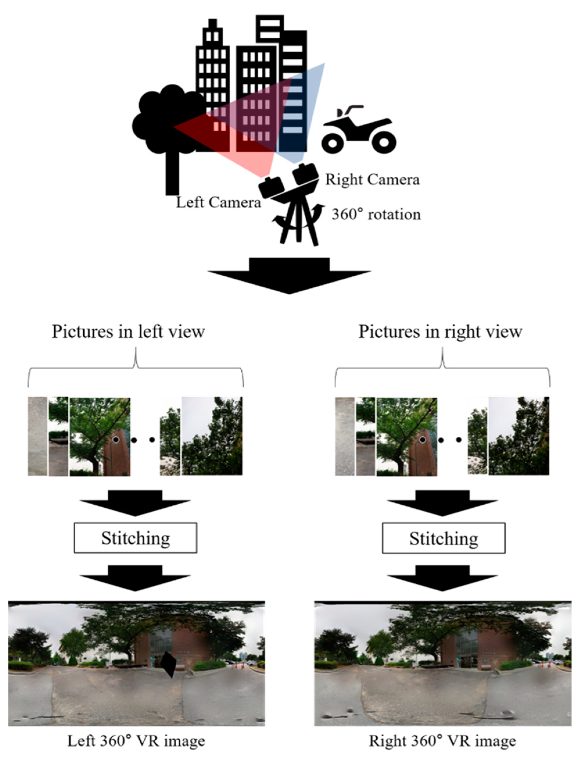
Figure 1. Procedure to make stereo 360 VR images consisting of left and right equi-rectangular projections (ERPs).
Applsci 11 02033 g001
Figure 2. Examples of left and right ERPs, where a hole is found in the left ERP: (a) B L l , B L c , B L r in the left ERP image; (b) B R l , B R c , B R r in the right ERP image.
Applsci 11 02033 g002
Figure 3. Process to detect the hole in an ERP image: (a) A stitched picture including a hole; (b) a black-and-white picture; (c) a binary image resulted from Step 2; (d) several contours of the candidate holes in the binary picture; (e) the map indicating the decided holes.
Applsci 11 02033 g003
Figure 4. Relationship between world coordinates and picture coordinates.
Applsci 11 02033 g004
Figure 5. Concealment process based on derived homography matrix: (a) A part of the left ERP; (b) A part of the right ERP.
Applsci 11 02033 g005
Figure 6. Homography matrixes H ( B L l B R l ) and H ( B L r B R r ) are calculated by applying the feature extraction algorithm and matching those feature points: (a) Example of feature matching when Homography matrix is H ( B L l B R l ) ; (b) Example of feature matching when Homography matrix is H ( B L r B R r ) .
Applsci 11 02033 g006
Figure 7. Flowchart of the proposed algorithm.
Applsci 11 02033 g007
Figure 8. Equirectangular projection images generated from test sets to evaluate different methods. (a) Laboratory, (b) Brick Road, (c) Alleyway, (d) Tree, (e) Bench, (f) Street, (g) Hallway, and (h) Mozart Hall.
Applsci 11 02033 g008
Figure 9. ERP images including holes and the concealed regions, where the holes are concealed by the proposed algorithm.
Applsci 11 02033 g009
Figure 10. Example of reference picture and the original picture with an artificial hole for test set Mozart Hall: (a) Reference picture with no hole; (b) Original picture with a hole.
Applsci 11 02033 g010
Figure 11. Concealed images resulting from various algorithms for test set Mozart Hall: (a) Result from Bertalmio [16]; (b) Result from Telea [17]; (c) Result from Criminisi [18]; (d) Result from Liu [19]; (e) Result from Gilisoft Stamp Remover [33]; (f) Result from Theinpaint [34]; (g) Result from simple copy; (h) Result from proposed method.
Applsci 11 02033 g011
Figure 12. Example of reference picture and the original picture with a large artificial hole for test set Hallway: (a) Reference picture with no hole; (b) Original picture with a hole.
Applsci 11 02033 g012
Figure 13. Concealed images resulting from various algorithms for a large hole for test set Hallway: (a) Result from Bertalmio [16]; (b) Result from Telea [17]; (c) Result from Criminisi [18]; (d) Result from Liu [19]; (e) Result from Gilisoft stamp remover [33]; (f) Result from Theinpaint [34]; (g) Result from simple copy; (h) Result from proposed method.
Applsci 11 02033 g013aApplsci 11 02033 g013b
Figure 14. Concealed image results from various algorithms for a hole generated during stitching procedure for test set Laboratory: (a) Original left and right ERPs with hole; (b) Left and right ERPs result by Bertalmio [16]; (c) Left and right ERPs result by Telea [17]; (d) Left and right ERPs result by Criminisi [18]; (e) Left and right ERPs result by Liu [19]; (f) Left and right ERPs result by Gilisoft stamp remover [33]; (g) Left and right ERPs result by Theinpaint [34]; (h) Left and right ERPs result by the proposed method.
Applsci 11 02033 g014aApplsci 11 02033 g014b
Table 1. Comparison between performances of various methods for outdoor pictures (Mozart Hall).
MethodSSIMPSNR (dB)Time (s)
Bertalmio [16]0.648319.698212.9177
Telea [17]0.632016.515513.1796
Criminisi [18]0.440617.080430346
Liu [19]0.238117.3725N/A
Gilisoft [33]0.742724.63472.1600
Theinpaint [34]0.770125.005828.1900
Simple copy0.619621.17930.0160
Proposed algorithm0.795425.44797.3261
Table 2. Performances of proposed method according to the size of the neighboring blocks for outdoor pictures (Mozart Hall).
Width RatioSSIMPSNR (dB)Time (s)
1.00.749124.15255.4439
1.20.758524.43556.3663
1.50.795425.44797.3261
1.750.761424.65538.0263
2.00.598619.86818.8201
Table 3. Comparison between performances of various methods for indoor pictures (Hallway) having a large hole.
MethodSSIMPSNR (dB)Time (s)
Bertalmio [16]0.715318.692815.7136
Telea [17]0.734318.031516.3712
Criminisi [18]0.569118.611362791
Liu [19]0.351116.1611N/A
Gilisoft [33]0.748723.51760.5500
Theinpaint [34]0.758522.56666.3600
Simple copy0.654416.92610.2273
Proposed algorithm0.772123.80208.8516
Table 4. Performances of proposed method according to size of neighboring blocks for indoor picture (Hallway) having a large hole.
Width RatioSSIMPSNR (dB)Time (s)
1.00.603115.84336.7485
1.20.647618.31337.6910
1.50.772123.80208.8516
1.750.650517.62639.3063
2.00.665618.75629.9974
Publisher’s Note: MDPI stays neutral with regard to jurisdictional claims in published maps and institutional affiliations.