Article

A Collaborative Control Method of Dual-Arm Robots Based on Deep Reinforcement Learning

School of Mechanical, Electrical & Information Engineering, Shandong University, Weihai 264200, China
*
Author to whom correspondence should be addressed.
Appl. Sci. 2021, 11(4), 1816; https://doi.org/10.3390/app11041816
Submission received: 6 January 2021 / Revised: 10 February 2021 / Accepted: 16 February 2021 / Published: 18 February 2021

Abstract

:
Collaborative control of a dual-arm robot refers to collision avoidance and working together to accomplish a task. To prevent the collision of two arms, the control strategy of a robot arm needs to avoid competition and to cooperate with the other one during motion planning. In this paper, a dual-arm deep deterministic policy gradient (DADDPG) algorithm is proposed based on deep reinforcement learning of multi-agent cooperation. Firstly, the construction method of a replay buffer in a hindsight experience replay algorithm is introduced. The modeling and training method of the multi-agent deep deterministic policy gradient algorithm is explained. Secondly, a control strategy is assigned to each robotic arm. The arms share their observations and actions. The dual-arm robot is trained based on a mechanism of “rewarding cooperation and punishing competition”. Finally, the effectiveness of the algorithm is verified in the Reach, Push, and Pick up simulation environment built in this study. The experiment results show that the robot trained by the DADDPG algorithm can achieve cooperative tasks. The algorithm can make the robots explore the action space autonomously and reduce the level of competition with each other. The collaborative robots have better adaptability to coordination tasks.

1. Introduction

The rapid development of deep reinforcement learning (DRL) has provided new ideas for robot control strategies [1,2,3]. The “QT-Opt” model proposed by Google Brain uses an end-to-end reinforcement learning algorithm to control the physical mechanical arm to perform a grasping task, and the success rate in the new object grasping task reaches 96% [4]. Researchers from the University of California, Berkeley Artificial Intelligence Lab proposed a method, which uses the virtual image generated by the variational auto-encoder as the task target. The agent can prepare to solve different tasks by setting its own goals, practicing complex behaviors, and learning the surrounding environment without any additional supervision sources [5]. By modeling the quadruped robot accurately and using the deep reinforcement learning algorithm, Hwangbo et al. directly applied the controller trained in the simulation environment to the real ANYmal robot, which made the quadruped robot have faster movement speed and recovery ability from falling [6]. However, single-arm robots have limitations in terms of operation and control. The dual-arm robots with coordinated operation and good human–machine collaboration functions demonstrate obvious superiority [7].
When a dual-arm robot cooperatively grasps an object, the controller will form a closed-loop chain structure. The position and the velocity of the end effector for each mechanical arm are constrained at the same time. The movement of each arm is always synchronized with the object. The state variables of the system are highly coupled [8,9]. These increase the difficulty of controller design. At present, the cooperative control strategies of multi-arm cooperating robots are mainly divided into a master–slave control strategy and hybrid position/force control strategy. The former is to plan the trajectory of the master manipulator according to the corresponding control target, and the slave manipulator plans the trajectory with the trajectory of the master manipulator as the constraint condition [10]. The latter decouples the position control from the force control by decomposing the state of the end effector and the task space where the constraint environment is located, to improve the speed and accuracy of position/force tracking [11,12]. However, the traditional control strategies of the manipulator are mostly based on the precise mathematical model based on tasks and have poor adaptability. When the tasks or environment changes, the control effect will be greatly reduced or even out of control.
The great success of deep reinforcement learning (DRL) prompted researchers to turn their attention to the multi-agent field, and integrated DRL method into Multi-Agent System, aiming at completing many complex tasks in a multi-agent environment, which gave birth to multi-agent deep reinforcement learning (MDRL) [13]. The breakthrough of multi-agent deep reinforcement learning provides a new method for multi-robot collaborative control, especially for the grasping objects that needed two-arm cooperation [14]. According to the communication mode between agents, the current MDRL methods are roughly divided into three types. The first method is to extend the single-agent DRL algorithm directly to the multi-agent environment. Each agent interacts with the environment independently and forms its behavior strategy. There is no communication association between agents [15,16]. The second is to establish an explicit communication mechanism between agents (such as communication mode, communication time, communication objects, etc.), and gradually determine and improve the communication mechanism during the learning process. After the training, each agent needs to make behavior decisions according to the information transmitted by other agents [17]. The third is not to directly establish explicit communication rules among multi-agents, but to use some theories in traditional multi-agent reinforcement learning to make agents learn the cooperative strategy [18,19]. The first method is easy to implement and has inherent advantages in scalability. However, because there is no communication between agents, each agent regards other agents as a part of the environment. From an individual point of view, the environment is constantly changing, which seriously affects the stability and convergence of the strategy. The advantage of the second method lies in that the channels established between agents can enable agents to learn better collective strategies, but its disadvantages are that there are many parameters needed to establish the channels, and the design architecture of the algorithm is more complex. Compared with other algorithms, the multi-agent deep deterministic policy gradient algorithm (MADDPG) can be applied to both cooperation and competitive environments. At the same time, during centralized training, the observations and strategies of other agents can be used to speed up the training process. The algorithm is more robust and has more application scenarios.
In order to mitigate the problem of difficult modelling and poor portability in the dual-arm robot cooperative control, the dual-arm deep deterministic policy gradient algorithm was proposed. This algorithm is based on the MADDPG algorithm. The robotic arms are controlled by two agents, and the strategy of each agent is independent of the other. During the training, we use Critics, which can observe the whole situation, to guide the training of the Actor. However, during the test, in order to avoid competition between two agents, Actors can also observe the whole situation and take action. The observations and actions between the two agents are shared, and the Hindsight Experience Replay algorithm (HER) [20] is used to solve the problem of sparse rewards. Experiments show that the dual-arm deep deterministic policy gradient algorithm can improve the speed of learning from sparse reward signals, and the dual-arm robot trained by this algorithm can achieve cooperative tasks.

2. Preliminary Knowledge

2.1. Hindsight Experience Replay

The problem of sparse reward has always been the core issue that deep reinforcement learning faces in solving practical tasks [21,22]. In supervised learning, supervised signals are provided by training data. In reinforcement learning, rewards play the role of supervising signals, and agents optimize strategies based on rewards. The problem of reward sparseness will cause the algorithm to iterate slowly and even converge difficultly [23]. In the collaborative task of the robotic arm, the robot can only obtain the reward after successfully completing a series of complex posture control to grab the target. Failure to succeed in any step in the training progress will lead to failure to obtain the reward [24,25].
Hindsight Experience Replay has been introduced to learn policies from sparse rewards, especially for robot manipulation tasks [26]. The rationale of HER is to replay each trajectory with an arbitrary goal. In this way, when the agent fails to achieve the desired goal in the episode, the additional goal can be used instead of the original desired goal, and then the reward is recalculated according to the new goal to provide experience for the agent. HER improves the sample efficiency in the sparse reward DRL algorithm and can be used in combination with any off-policy reinforcement learning algorithm [27]. The key of the HER algorithm is how to construct the replay buffer [28], which includes two steps. Firstly, a fixed size queue where each entry is a 5-tuple and is randomly selected from M sequences, and the initial state s 0 and goal g are defined. The agent produces an action based on the current state and goal g. The action formula is shown as follows:
a t π ( s t | | g )
where s t and g are the current state and goal, a t is the selected action, and π is the behavior strategy. Then, the reward can be calculated as follows:
r t r ( a t , s t | | g )
The sample ( s t , a t , r t , s t + 1 , g ) will be stored in the replay buffer. Then, a complete agent’s experience sequence at each time is sampled based on the actual goal g. Secondly, the reward is recalculated using a new goal g’. The reward formula is as follows:
r r ( a t , s t | | g )
The same data structure as the normal training transitions is constructed. The obtained transitions ( s t , a t , r , s t + 1 , g ) are also stored in the replay buffer. Then, the new experience transitions are obtained by changing the goal. After the replay buffer is constructed, the agent can be trained through some off-policy reinforcement learning algorithms.
There are four main methods to obtain new goals, including: final, future, episode, and random. The final strategy is to take the final state in each episode as the new goal. The future strategy is to replay the successive states with k random states, which come from the same episode after the current time. The episode strategy is to replay the special states with k random states, which come from the same episode as the transition being replayed. The random strategy is to replay the special states with k random states that appeared so far in the whole training procedure. A new experience sample can be obtained based on the first goal generation strategy. The last three strategies have a hyper-parameter k which controls the ratio of HER data to those coming from normal experience replay in the replay buffer, and k new experience transitions can be generated from one original sample.

2.2. Multi-Agent Deep Deterministic Policy Gradient

Traditional reinforcement learning algorithms are poorly suited to multi-agent environments. One issue is that during the training process, each agent′s policy is changing, and the environment becomes non-stationary from the perspective of any individual agent. This presents learning stability challenges and prevents the use of past experience replay. On the other hand, policy gradient methods usually have very high variance when multiple agents need efficient coordination.
The MADDPG algorithm aims to solve the multi-agent control strategy in a variety of cooperative and competitive multi-agent environments, which is an extension of the Deep Deterministic Policy Gradient (DDPG) [29]. DDPG uses the Actor–Critic [30] framework, which includes two neural networks: a target policy (the actor) μ : S A and an action value function approximator (the critic) Q : S × A R . The actor select actions based on the current observations. The critic′s job is to approximate the actor′s action-value function Q μ . MADDPG adopts the framework of centralized training with decentralized execution. The critic can obtain extra information about the policies of other agents, while the actor only obtains local information. During the execution phase after training is completed, only the local actors are used to act in a decentralized manner.
More specifically, suppose that there are N agents in the system. The set of all policies is μ = { μ 1 , , μ N } , which is parameterized by θ = { θ 1 , , θ N } . Every policy is represented by one neural network. Each agent’s policy only depends on its own observations, which means a i = μ i ( o i ) , and no structural assumptions are made on the communication methods between agents. The action value function Q i μ ( x , a 1 , , a N ) describes the expected return after taking the actions, a 1 , , a N , in state x . In the simplest case, x could consist of the observations of all agents, x = ( o 1 , , o N ) . The critic network parameters are updated by minimizing the following loss:
L ( θ i ) = E x , a , r , x [ ( Q i μ ( x , a 1 , , a N ) y ) 2 ] , y = r i + γ Q i μ ( x , a 1 , , a N ) | a j = μ j ( o j )
where, y is the target value, γ [ 0 , 1 ] is a discount factor, and μ = { μ θ 1 , , μ θ N } is the set of target policies with delayed parameters θ i . The parameters of the action network are updated based on the gradient descent method. Using the Q function defined previously, the gradient of the policy can be written as:
θ i J ( μ i ) = E x , a D [ θ μ μ i ( a i | o i ) a i Q i μ ( x , a 1 , , a N ) | a i = μ i ( o i ) ] .
where, D is a distribution over transitions ( x , a , r , x ) contained in the replay buffer.

3. Dual-Arm Deep Deterministic Policy Gradient Algorithm

The problem setup is as follows. Given a cooperative task, the dual-arm robot must learn how to collaborate to complete the task through a sequence of actions. This process is controlled by two agents in the continuous action space. The policy of each agent changes during training, resulting in a non-stationary environment. Agents not only adapt to the state of the environment but also cooperate with other agents’ action strategies. Based on HER and MADDPG, a dual-arm deep deterministic policy gradient algorithm (DADDPG) was proposed for collaborative control of dual-arm robots. Figure 1 shows the block diagram of the DADDPG algorithm.
The DADDPG algorithm uses two agents to control two robotic arms, and each agent is trained using the DDPG algorithm. In order to encourage agents to reduce competition and increase collaboration in overlapping action spaces, the two agents share observations and actions with each other. Each agent adjusts its own action strategy according to the output of the other one and finally achieves cooperation.
More specifically, each of the two mechanical arms has an agent, and they interact within the same environment. The training algorithm for each agent is DDPG. At each timestep, each agent i takes an action a i to interact with the environment; the joint action leads to a new state, and each agent i receives their own separate observations o i . However, in order to achieve cooperation between the two arms, a collaborative mechanism of rewarding coordination and punishing competition is introduced. The agents can share the states and actions of each other. Namely, each agent’s actor can obtain a global observation vector x = ( o 1 , o 2 ) . For each agent i, the algorithm maintains two actor and critic functions. One of the actor functions μ i ( x i | θ i μ ) is the current policy to select an action based on the observation o i , and one of the critics Q ( x , a | θ i Q ) is learned using the Bellman equation as in MADDPG. The other actor and critic networks, μ i ( x i | θ i μ ) and Q ( x , a | θ i Q ) , respectively, are a copy of them. They are used to calculating the target values. The weights of these target networks are updated by slowly tracking the learned networks. At the same time, samples from a noise serial N are added to the actor policy to treat the problem of exploration. Agent i makes an action a i t based on the output of its actor network and random noise, and obtains observation o i t + 1 which is a g i t generated by a i t ( a g represents the state that the agent has reached, which can also be called the achieved local goal). A replay buffer is used to ensure the samples are independently and identically distributed. The replay buffer is a cache R, which has a finite size. At each step, the actor and critic are updated by sampling a minibatch uniformly from the buffer.
To improve the convergence of the algorithm, the samples are processed using the HER algorithm. Mini-batch size groups of data are randomly extracted from the replay buffer. The original goal is recorded as g, and the goal replacement is performed sequentially. Take a sample ( x i , a i , g i ) from { x 1 , a 1 , g 1 , a g 1 , , x t , a t , g t , a g t } . In this paper, the reward was not given when the sample was saved from the episode the first time, because the reward needs to be calculated based on the reward function. This solution dramatically increases efficiency and saves memory. The method to create a new goal is the future strategy. Let the sampling time be step i; the original goal g would be replayed by a g in k ( k = 4 ) steps, which comes from the same episode and was observed after step i. That means g a g j , j [ i + 1 , T ] , where T was the set length of time. After the new goal g , the reward r is recalculated and the new tuple ( Χ t | | g , a t , r , Χ t + 1 | | g ) is stored in the replay buffer. The replay buffer at this time records the experience of all agents. At each timestep, the actor and critic are updated by sampling a minibatch uniformly from the buffer. The pseudo-code of the DADDPG algorithm can be described as follows:
Algorithm 1. Dual-arm deep deterministic policy gradient algorithm.
  • For each agent i:
    • randomly initialize critic network Q i ( x , a 1 , a 2 | θ i Q ) and actor μ i ( o i | θ i μ ) with weights θ i Q and θ i μ
    • Initialize target network Q i and μ i with weights θ i Q θ i Q , θ i μ θ i μ
  • Initialize replay buffer: R
  • forepisode = 1 to M do
  •  Initialize a random process N for action exploration
  •  Sample a goal g and an initial state x 1
  • for t = 1 to T do
  •   For each agent i, select action a i t = μ i ( o i | θ i μ ) + N according to the current policy and exploration noise
  •   Execute actions a t = ( a 1 t , a 2 t ) and observe new state x t + 1
  • end for
  • for t = 1 to T do
  •   For each agent i, calculate reward r i t : = r ( x t , a i t , g )
  •   Store the transition ( x t g , a t , r t , x t + 1 g ) in R
  •   Sample a set of additional goals for replay G: = X (current episode)
  •   for g G do
  •    For each agent i, r i t :   = r ( x t , a i t , g )
  •    Store the transition ( x t g , a t , r t , x t + 1 g ) in R
  •   end for
  • end for
  • for t = 1 to T do
  •   for agent i = 1 to 2 do
  •    Sample a random minibatch of N transitions ( x j , a j , r j , x t + 1 , j ) from R
  •    Set y j = r i j + γ Q i ( x t + 1 , j , a 1 , a 2 | θ i Q ) | a k = μ k ( o k j | θ k μ )
  •    Update critic by minimizing the loss:
    L = 1 / N j ( y j Q i ( x j , a 1 , a 2 | θ i Q ) ) 2
  •    Update the actor policy using the sampled policy gradient
    θ i J 1 / N j a i Q i ( x j , a 1 j , a 2 j | θ i Q ) | a i = μ i ( o i j ) θ i μ μ i ( o i j | θ i μ )
  •   end for
  •   Update target network parameters for each agent i:
    θ i Q τ θ i Q + ( 1 τ ) θ i Q
    θ i μ τ θ i μ + ( 1 τ ) θ i μ
  • end for
  • end for
In practice, the data generated in an episode are saved in the replay buffer. The data include the states x t and actions a t at each moment, and are stored in chronological order. The set length of time is T = 50 and the number of elements in the sequence is N = 1 , 000 , 000 . The replay buffer can be large, allowing the algorithm to benefit from learning across a set of uncorrelated transitions. When the replay buffer overflows, the oldest transitions will be discarded. If the mission has been completed within time T, the round episode will be terminated early. If the mission is not completed within 50 timesteps, this round will also be forcibly terminated. This is to reduce the difficulty of exploring space.

4. Experiments

4.1. Simulation Experiments

In this paper, dual-arm robot simulation environments were created in Gym [31]. In all experiments, we used two UR3 arms, which each had a two-fingered parallel gripper. The robot was simulated using the MuJoCo physics engine [32]. The whole training procedure was performed in simulation. The networks of actors and critics in the algorithm had 3 hidden layers with 256 hidden units in each layer. Hidden layers used the ReLu activation function. They were trained by using Adam as the back propagation of the optimizer.
In the simulation, the core tasks of the robots are to obtain observations and select actions. The goal is independent of any physical characteristics. The observation results are described by the position information between the grippers and the object, including the three-dimensional spatial coordinates of the grippers, the spatial coordinates of the object, the coordinates of the object relative to the grippers, the state of the gripper, the attitude of the object, the moving speed of the object, the rotating speed of the object, the speed of the gripper, and the speed of the gripper’s fingers. Note that different tasks have different initialization settings, which will change the data dimensions of the observations. Action is represented by a vector containing eight elements: a = [ a 1 , a 2 , a 3 , a 4 , a 5 , a 6 , a 7 , a 8 ] . Each element in the vector is normalized in the range: a i [ 1 , 1 ] . The first four elements control the left arm gripper, and the last four elements control the right arm gripper. The four elements of the left arm are taken as an example here. The first three elements represent the displacement of the gripper on the X, Y, and Z axes, and the fourth element represents the distance that a single finger moves in the two-fingered parallel gripper.
Three different tasks are executed in the experiments:
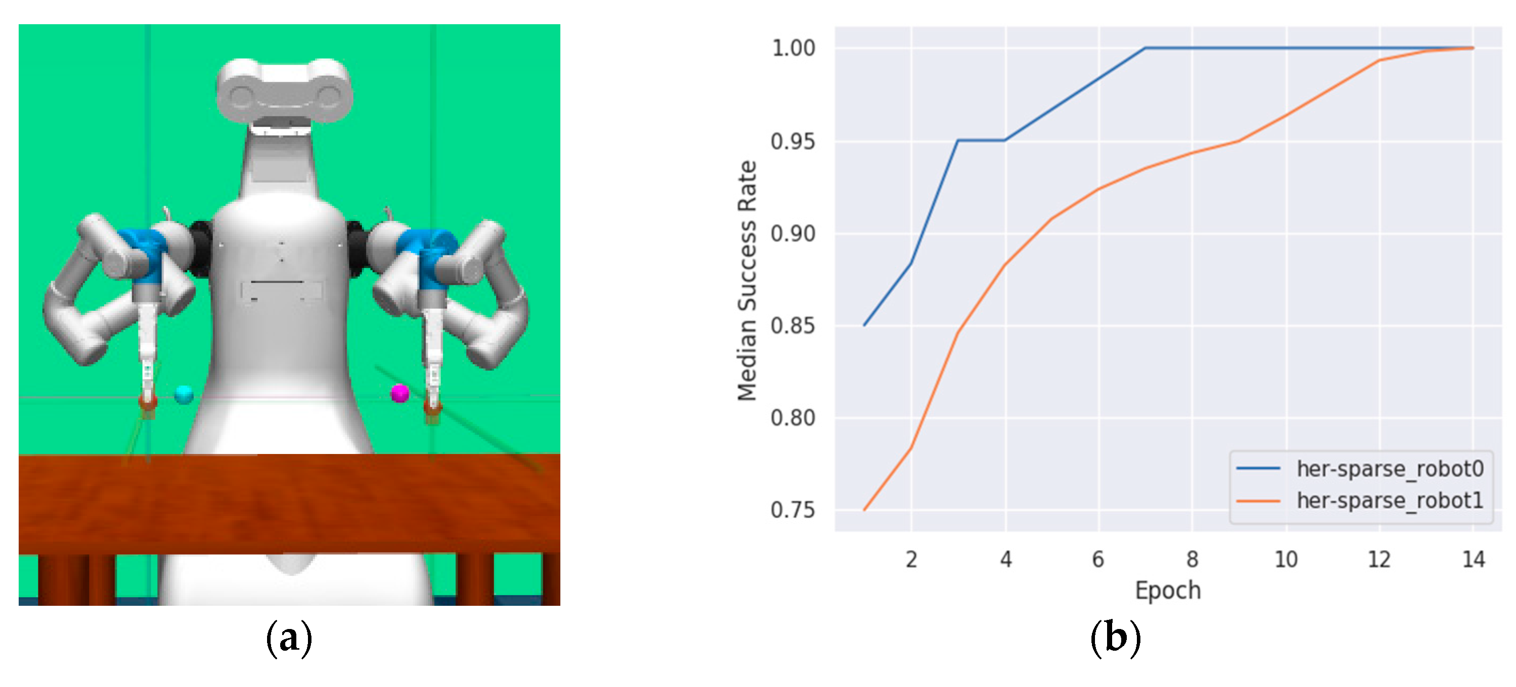
Reach: The task is to move the end grippers of the robot arms to the left and right target positions, as shown in Figure 2a. There are no objects in this scene, and the observation data related to the objects are all set to zero. The fingers of each robotic arm are locked to prevent grasping. The reward function is calculated by the distance between the grippers and the target positions. An episode is successful if the distance between the gripper and the desired target is less than 2 cm. The closer the proximity, the greater reward the robots will obtain. The learning curves are shown in Figure 2b. The abscissa is the number of training rounds, and the ordinate is the average success rate of 10 tests. The convergence speed varies depending on the difficulty of the task. In this scenario, no exploration period is needed, because each movement of the robotic arms can be converted into a positive training sample.
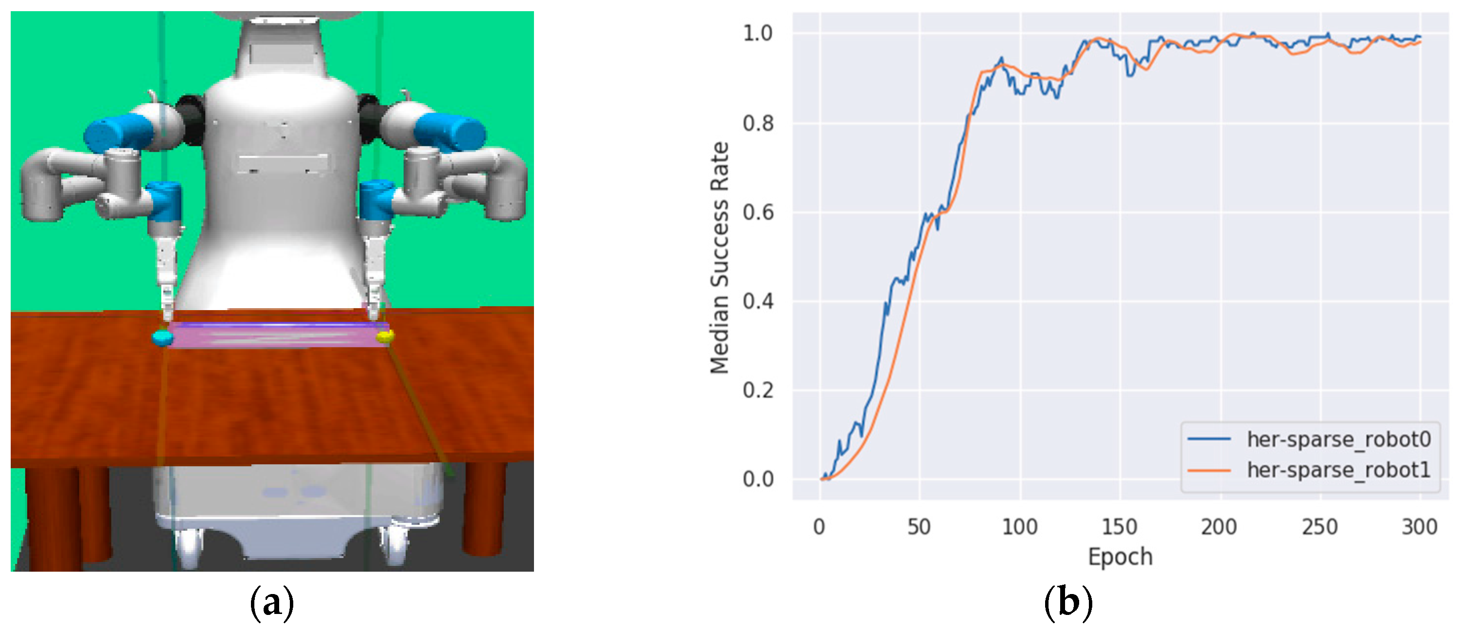
Push: In this task, a block is placed on a table in front of the dual-arm robot. The task of the robotic arms is to cooperatively move the block to the target location on the table, as shown in Figure 3a. Since the grippers need to grab the object in this scene, its position and orientation will change according to the block. Similar to the Reach scene, it is not necessary to consider the movement of fingers. The reward function is set as the distance from the left and right ends of the object to the target points. An episode is successful if the distance between the block and the desired target is less than 5 cm. In this scenario, the object is not scalable, so the agent must cooperatively push the object. The robot cannot learn knowledge in the initial exploratory period. Because the random motion of the robotic arms does not change the position of the object during the initial exploration phase, the robot cannot obtain effective experiences. Once a robot arm changes the position of the object, reinforcement learning will begin to reinforce this action sequence, so that it learns quickly after this action until the task is completed. Figure 3b shows the learning curves.
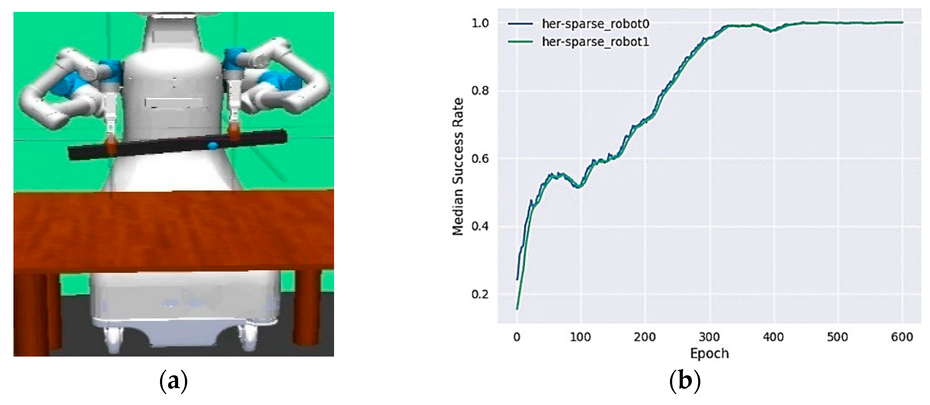
Pick up: This task is similar to the Push scenario but the target positions are in certain areas above the table and the fingers are not locked, as shown in Figure 4a. The reward function is set based on the distance from the object to the target positions. An episode is successful if the distance between the gripper and the desired target is less than 5 cm. The robot cannot learn knowledge in the initial exploration stage, but can quickly accumulate experience after it changes the position of the object. However, this task is more complicated than the first two. The agents need to control the grippers to move over the two ends of the object, and then control the fingers to open and close for grasping. During the ascending process of median success rate, the relative motion of the two robot arms cannot drastically change, and the grippers cannot be released. Otherwise, the task will fail. Due to the addition of random noise, the dual-arm robot will appear uncoordinated. From Figure 4b, it is clear that the success rate fluctuates at the beginning of training, but the results eventually converge. According to the analysis of the experimental results, due to the difficulty of the task being different, the time for the algorithm to terminate training varies greatly.
We conducted experiments using the DADDPG algorithm in the simulation environment. For each training epoch in the experiment, 50 episode cycles (20 episode cycles in the Reach scene) were executed by two parallel agents in the environment and stored in the replay buffer, followed by 40 steps of optimization of the policy performed by Adam. After each training epoch, 10 test episodes were executed and the success rate was calculated. For the Reach, Push, and Pick up tasks, the difficulty of the tasks leads to different training rounds, but the DADDPG algorithm finally converges to the optimal result.
The gripping pot experiment was performed in order to verify the performance of the proposed algorithm, as shown in Figure 5a. A circle protrudes from the top of the object. The robot arms are trained based on the proposed algorithm. The robot can touch the reasonable point to grip the pot, and put the pot in a specified area. Figure 5b shows the robot arms are exploring to search the target object at the beginning stage. When they can touch the pot, the learning curve gradually increases as time goes on. However, gripping the pot is more difficult than touching it. The learning curve begins to oscillate with a small amplitude during the learning process because the arms try to grip the pot. With the refinement of the action strategy, the algorithm converges to the optimal solution. The simulation results show the model can be convergent for different tasks and has better generalization ability.

4.2. Physical Robot Control

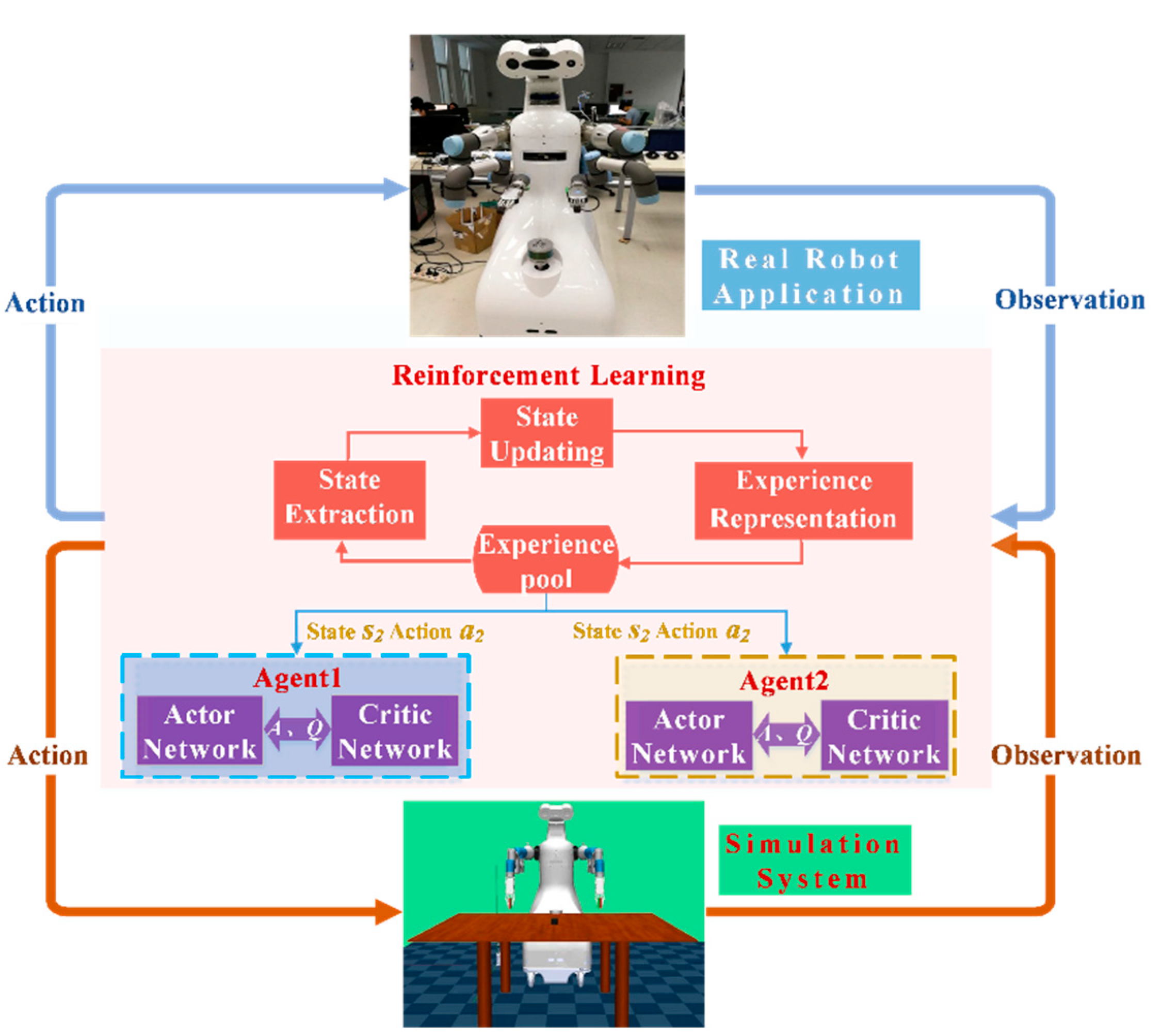
A control system is designed based on robot operating system (ROS) infrastructure for the dual-agent deep deterministic policy gradient algorithm. A Kinect camera is used to position the target based on a mask region convolutional neural network (Mask-RCNN) [33]. The special tasks are successfully implemented by the dual-arm robot in the simulation. The simulation condition is replaced by the physical environment to transfer the algorithm on the basis of the equivalence principle. The algorithm transferring architecture is shown in Figure 6.
ROS is a collection of tools, libraries, and conventions. Designing complex robot behavior will be simplified based on ROS, which is a flexible framework with a publish/subscribe communication mechanism between nodes. The robot models can be compatible with a wide variety of robotic platforms. The agent of the deep reinforcement learning algorithm is a server. The dual-arm robot sends the observation to an agent using ROS, and requires a service from the agent. The agent sends the control command back to the robot based on observation using the DADDPG algorithm. The control architecture is shown in Figure 7. The dual-arm robot can operate when it requires a decision service from a server. In this paper, two task scenarios are transferred to a physical robot: Reach and Pick up.
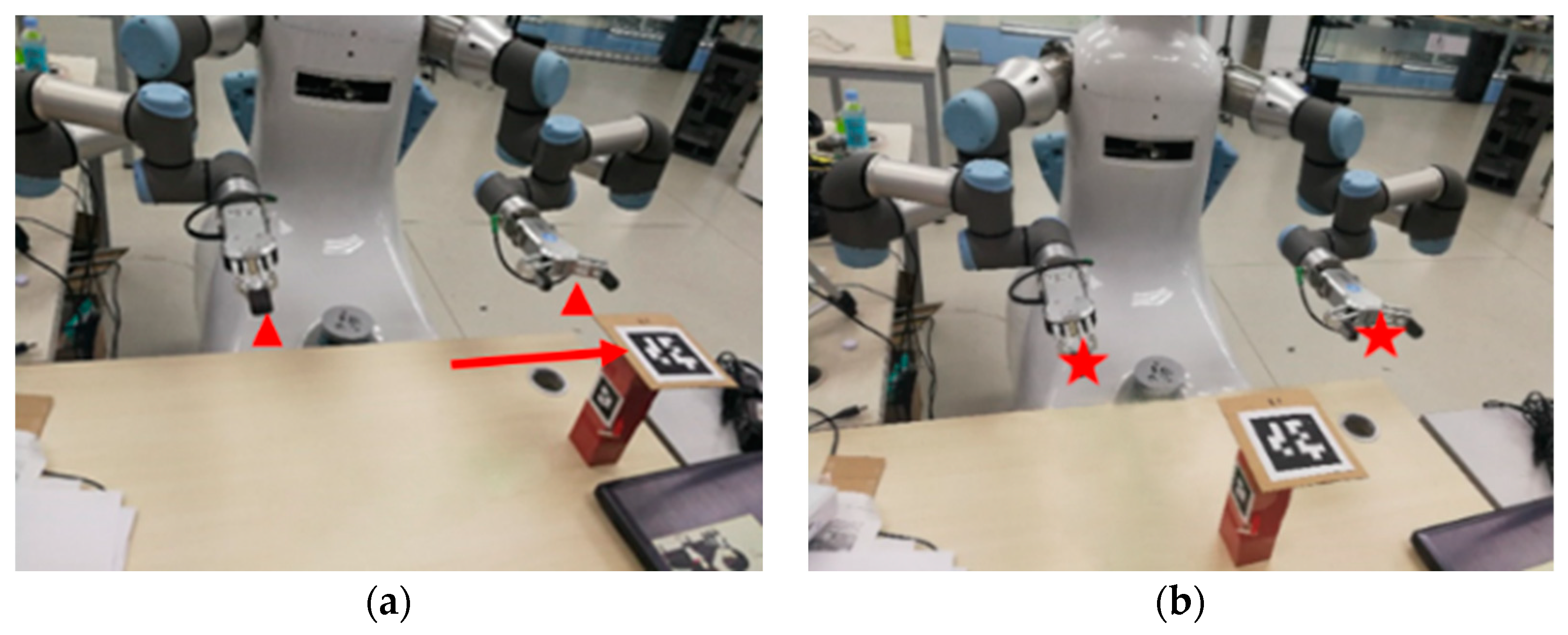
Reach: In this task, the gripper does not need to open and close. There are only three observations: the current gripper position, target point location, and the relative position of the fingers and the target position. The Python library “urx” is used to control the robotic arm, where the command “urrobot.getl()” can obtain the current pose of the gripper, including the 3D coordinates and pitch angle. The acquired pose takes the base of the robot as the reference coordinate system and needs to be converted to the absolute position with the ROS coordinate conversion tool. In this paper, Apriltags technology is used to complete the setting of target points. The image obtained by the camera is shown in Figure 8a. The two triangles represent the current position of the fingers and the QR code pointed to by the arrow is a picture in a special encoding format used by Apriltags. According to the pose of the QR code in the image, the Apriltags algorithm can calculate the position and orientation of the QR code in the camera coordinate system. In this article, the selected target points in the left and right directions are 10 cm above the QR code, as shown in Figure 8b. The agents need to control the two grippers to reach the target point.
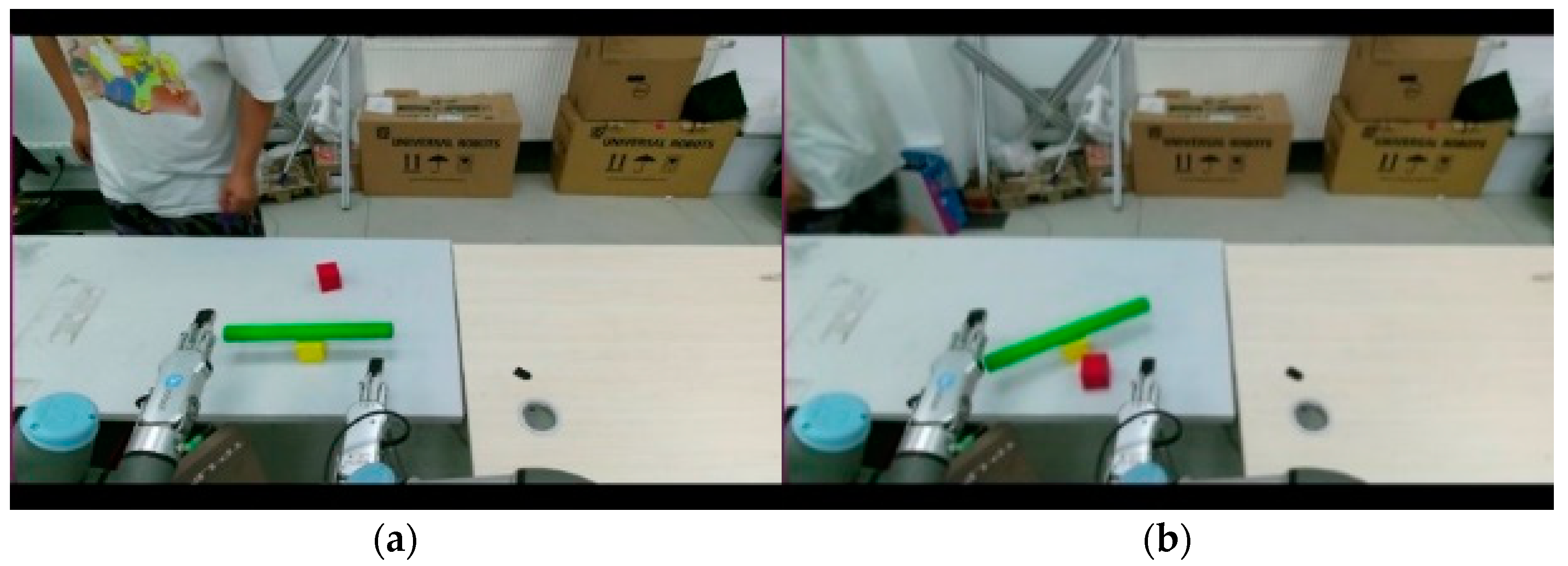
This paper uses the Mask-RCNN algorithm to output the label and pixel position of the target in the object recognition step. When making the dataset of the Mask-RCNN algorithm, it is necessary to annotate the labels and regions at the same time. Figure 9 shows the unlabeled images in the dataset containing thin rods at different positions and different angles, and then annotated the thin rods and colored squares using annotation software. The purpose of marking squares is to compare the accuracy of object recognition. The Mask-RCNN is trained by the dataset and packaged into an ROS node.
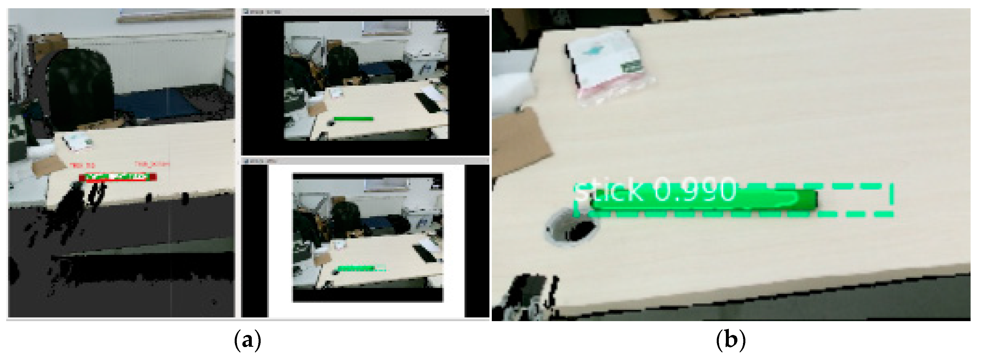
All experiments are performed on a computer equipped with GTX1080Ti GPU, and the release frequency at Kinect HD resolution is 30 Hz. In the actual test, Mask-RCNN can recognize the target in real time without obvious delay, as shown in Figure 10a. Figure 10b shows that the recognition result of the Mask-RCNN algorithm is “stick, 0.990”, including the Mask region, label, and confidence. It is clear that the Mask-RCNN algorithm can identify the approximate position of the thin rod, but it cannot locate it accurately. Overall, the two major reasons why the recognition is not accurate are not enough detailed annotation, and a lack of a dataset. In this paper, 100 pictures are collected, 80 of which are used as training sets and 20 as test sets.
Based on the target area identified by the Mask-RCNN algorithm, color threshold segmentation is used to discriminate each pixel in an area of about 15 pixels outside the target area. The two algorithms complement each other and improve the robustness and accuracy of target recognition. The result is shown in Figure 11.
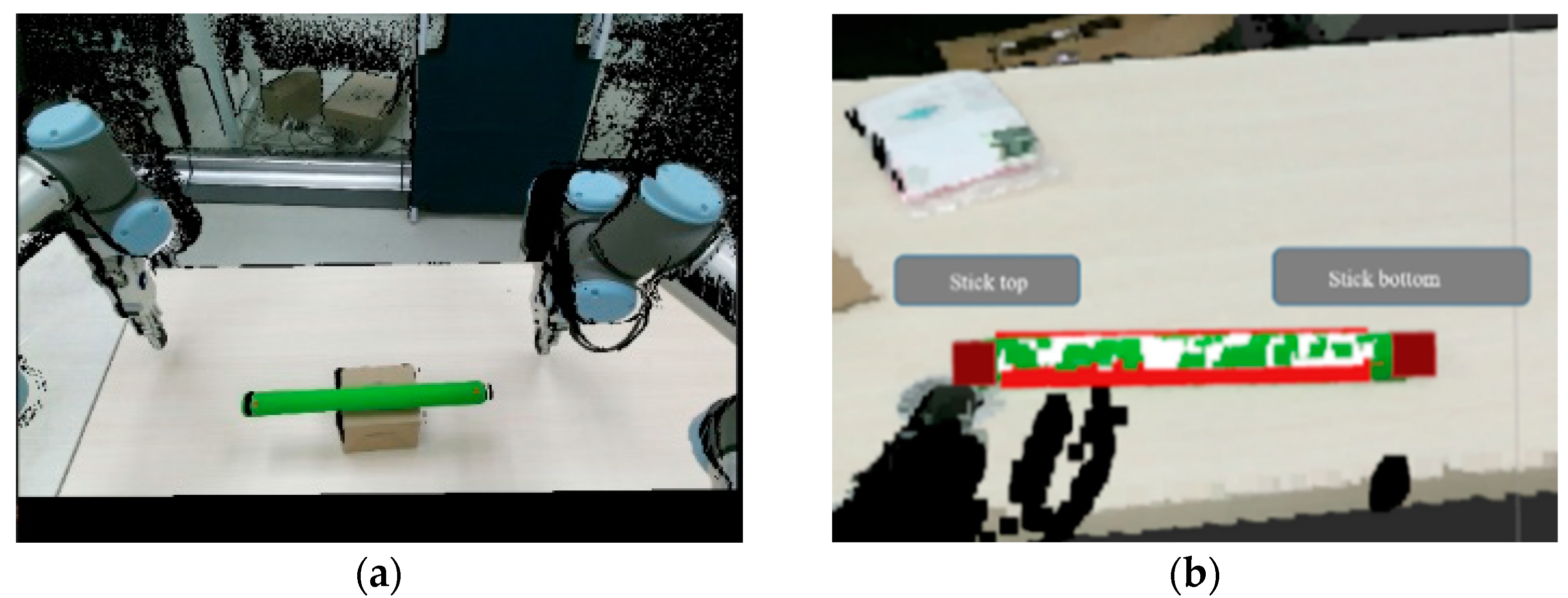
As shown in Figure 12a the threshold of the color is selected according to the pixel value of the thin green rod in the image, and the red and white parts in Figure 12b are the Markers displayed by RVIZ to assist in verifying the recognition results. The coordinates of both ends of the thin rod in the image are calculated, and are used as an index to find the corresponding point cloud coordinates to obtain the position of the thin rod.
Pick up: During this task, when the robot’s arms are close to the thin rod, the recognition of the thin rod will be incomplete because the joints of the arms shut out the view. The results show that the length of the thin rod is shortened, which leads to fluctuation of the spatial coordinates of the thin rod and makes the action value output by the algorithm unpredictable.
This article takes the following measures to alleviate the influence caused by occlusion: First, we increase the tilt angle of the wrist joint of the arm and approach the thin rod with a posture similar to “embracing”. Second, we calculate the center coordinates of the thin rod, and then deduce the positions of both ends. Third, we assume that the thin rod will not move without external force and its coordinates will remain unchanged until it is grasped. It is easy to obtain the coordinates of the unobstructed rod, and the position can be calculated according to the midpoint during the capture process. The observations in the simulation environment are customized according to the data types available to the physical robot. The simulation robot takes the lower right corner of the chassis as the reference origin, while the real robot takes the bottom center of the Frame as the reference origin, so it is necessary to transform the reference coordinate of the real robot into that of the virtual robot. With all the preparations completed, the master control program starts to operate. In this paper, it is set to acquire the observations every three seconds and request the Dual-UR3 service of ROS.
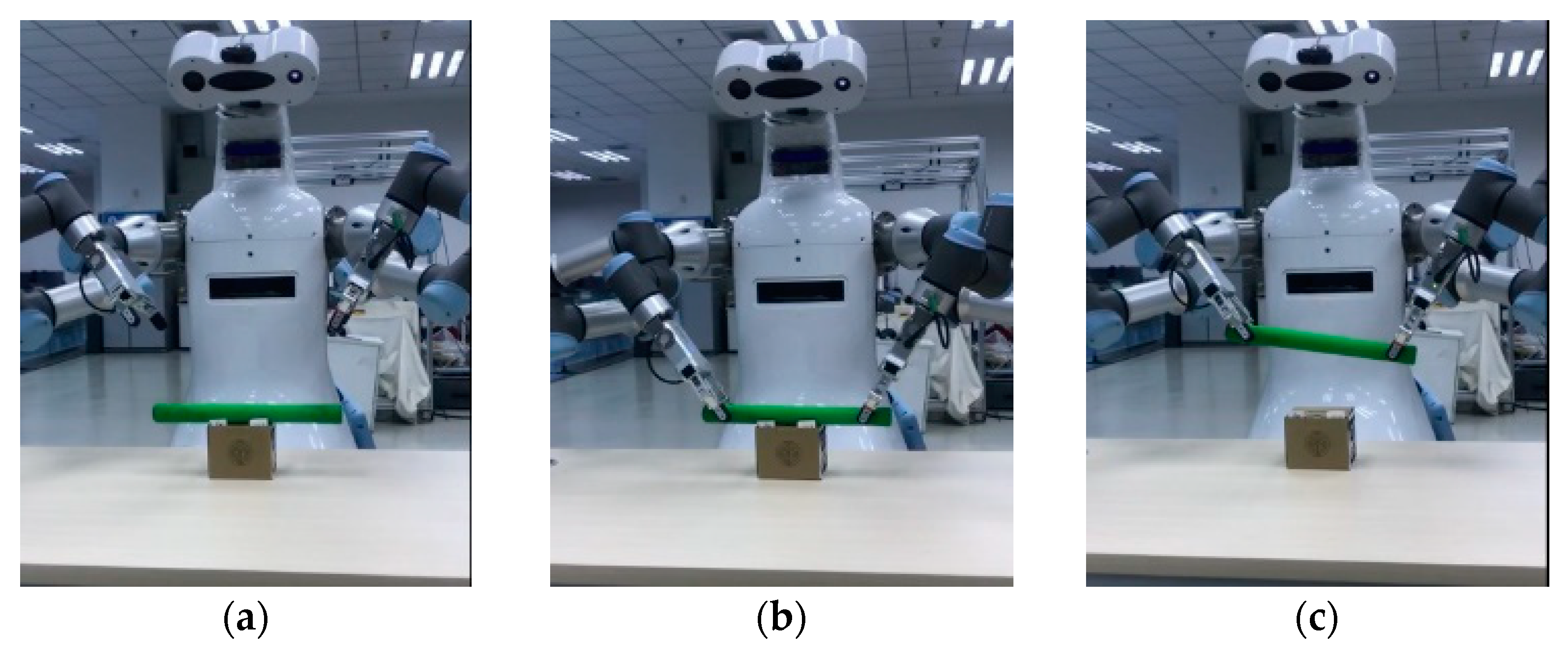
With all the preparations completed, the master control program starts to operate. In this paper, it is set to acquire the observations every three seconds and request the Dual-UR3 service of ROS. The action output is shown in Figure 13. The action is decomposed into two control signals, which are transmitted to the controllers of two arms through IP and executed at the same time. The dual-arm robot can complete the cooperative grasping task of lifting the thin rod to 15 cm, as shown in Figure 13.
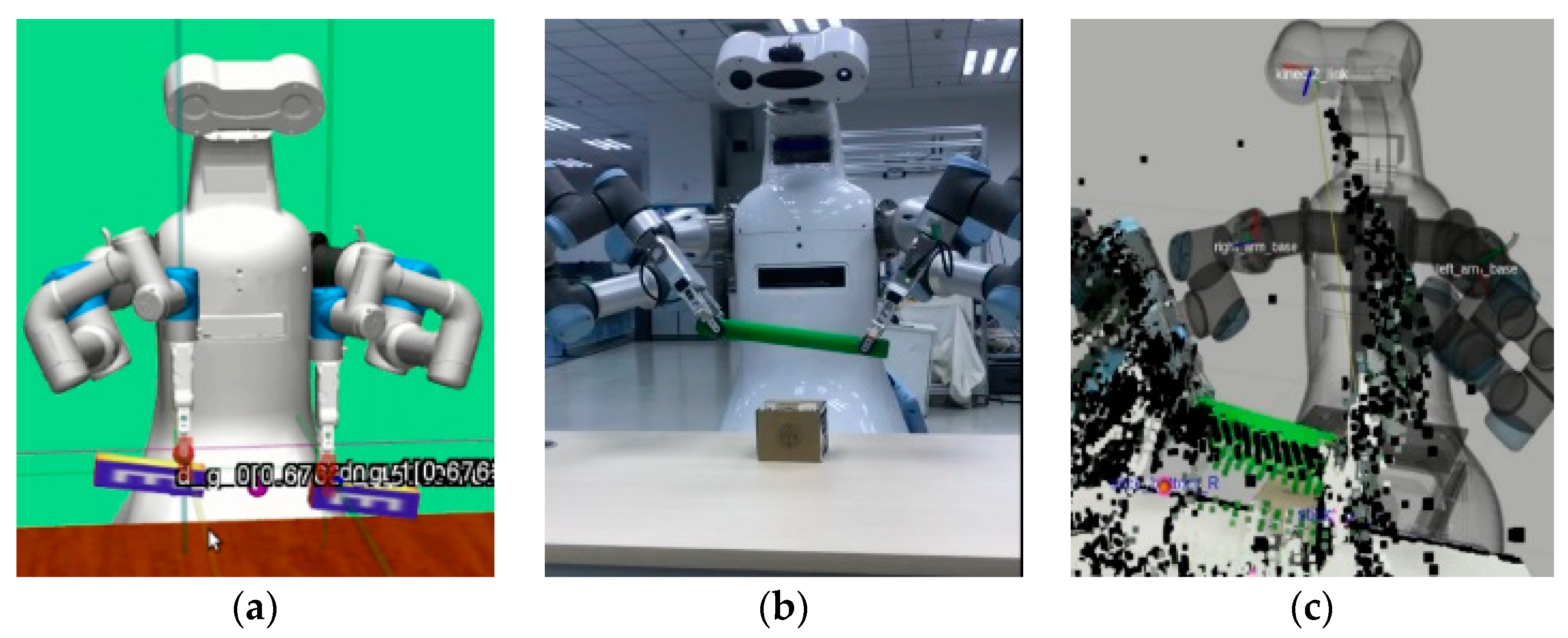
Figure 14 shows that the thin rod is slightly inclined when the task is completed, because the state is inclined when the task is accomplished in the simulation environment. The reasons for the tilt of the object are considered as follows: The first is the threshold setting of the reward function in the simulation environment. Setting the threshold too low will lead to slow convergence, while setting the threshold too high will lead to insufficient accuracy in completing tasks. Second, the calculation process of the reward function is instantaneous, and the agent will ignore it after a certain action receives a reward. The third is whether the reward function is scientific. The reward function determines the performance of the reinforcement learning algorithm to a great extent. This paper uses distance to judge the reward of the instantaneous state, which is not enough to describe the collaborative task completely. However, the three tilt states in Figure 14 also confirm to each other that the DRL algorithm is controlling the robot.

5. Conclusions

The DADDPG algorithm was proposed in combination with multi-agent deep reinforcement learning, and the HER algorithm was used to solve the problem of sparse robot rewards. Each robot arm has its own control strategy, which enhances robot collaboration by sharing observations and outputs between agents. This algorithm allows the robot to autonomously learn cooperative motion, and can complete simple collaborative tasks. A simulation was set up on the MuJoCo platform where an end-to-end policy is trained using the DADDPG algorithm. The proposed method is validated with three classic robotic control tasks (Reach, Push, and Pick up), and the separately designed Gripping pot experiment also shows that the algorithm has better generalization ability. The Mask-RCNN model for identifying a target block is regarded as a node of ROS, and the trained policies are regarded as the server of ROS. The policies are implemented directly in a physical robot to make decisions without any further training. Reach and Pick up tasks are realized on the real robot, which can command the robot arm to reach the target point to realize the Reach task, and can also accurately identify the target block, and command the two robotic arms to grab the block at the target point. In this process, mathematical modeling of the robot is avoided, and the adaptability of the robot to the external environment is improved. A few limitations to our approach remain. The current tasks are the most basic and simple. It is a worthy research direction to realize the cooperative ability of manipulators in a dynamic and changeable environment or under the condition that the object is blocked.

Author Contributions

Conceptualization, Q.L.; methodology, L.L. and Q.L.; software, L.L. and Q.L.; validation, L.L. and Q.L.; formal analysis, X.Y.; investigation, Q.X.; resources, Q.X.; data curation, X.Y.; writing—original draft preparation, Y.S., L.L. and B.P.; writing—review and editing, L.L. and B.P.; visualization, L.L. and Q.L.; supervision, Y.S.; project administration, Y.S.; funding acquisition, Y.S. All authors have read and agreed to the published version of the manuscript.

Funding

This research received no external funding.

Informed Consent Statement

Not applicable.

Acknowledgments

This work was supported by the National Natural Science Foundation of China under Grants (61973184, 61673245, 61803227), Independent Innovation Foundation of Shandong University under Grant 2018ZQXM005, The Development Plan of youth Innovation Team in colleges and Universities of Shandong Province under Grant 2019KJN011, and National Social Science Foundation of China under Grants (20ASH009).

Conflicts of Interest

The authors declare no conflict of interest.

References

  1. Arulkumaran, K.; Deisenroth, M.P.; Brundage, M.; Bharath, A.A. Deep Reinforcement Learning: A Brief Survey. IEEE Signal Process. Mag. 2017, 34, 26–38. [Google Scholar] [CrossRef] [Green Version]
  2. Ding, Z.; Huang, Y.; Yuan, H.; Dong, H. Introduction to reinforcement learning. In Deep Reinforcement Learning; Springer: Berlin/Heidelberg, Germany, 2020; pp. 47–123. [Google Scholar]
  3. Bhagat, S.; Banerjee, H.; Tse, Z.T.H.; Ren, H. Deep Reinforcement Learning for Soft, Flexible Robots: Brief Review with Impending Challenges. Robotics 2019, 8, 4. [Google Scholar] [CrossRef] [Green Version]
  4. Kalashnikov, D.; Irpan, A.; Pastor, P.; Ibarz, J.; Herzog, A.; Jang, E. Qt-opt: Scalable deep reinforcement learning for vision-based robotic manipulation. arXiv 2018, arXiv:180610293. [Google Scholar]
  5. Nair, A.V.; Pong, V.; Dalal, M.; Bahl, S.; Lin, S.; Levine, S. Visual reinforcement learning with imagined goals. arXiv 2018, arXiv:1807.04742. [Google Scholar]
  6. Hwangbo, J.; Lee, J.; Dosovitskiy, A.; Bellicoso, D.; Tsounis, V.; Koltun, V. Learning agile and dynamic motor skills for legged robots. Sci. Robot. 2019, 4, 1–13. [Google Scholar]
  7. Weng, C.-Y.; Chen, I.-M. The Task-Level Evaluation Model for a Flexible Assembly Task with an Industrial Dual-Arm Robot. In Proceedings of the 2017 IEEE International Conference on Cybernetics and Intelligent Systems (CIS) and IEEE Conference on Robotics, Automation and Mechatronics (RAM), Ningbo, China, 19–21 November 2017; pp. 356–360. [Google Scholar]
  8. Makris, S.; Tsarouchi, P.; Matthaiakis, A.-S.; Athanasatos, A.; Chatzigeorgiou, X.; Stefos, M.; Giavridis, K.; Aivaliotis, S. Dual arm robot in cooperation with humans for flexible assembly. CIRP Ann. 2017, 66, 13–16. [Google Scholar] [CrossRef]
  9. Wan, W.; Harada, K. Developing and Comparing Single-Arm and Dual-Arm Regrasp. IEEE Robot. Autom. Lett. 2016, 1, 243–250. [Google Scholar] [CrossRef] [Green Version]
  10. Leksono, E.; Murakami, T.; Ohnishi, K. On hybrid position/force cooperative control of multimanipulator based on workspace disturbance observer. In Proceedings of the 1996 IEEE IECON 22nd International Conference on Industrial Electronics Control, and Instrumentation, Taipei, Taiwan, 9 August 1996; pp. 1873–1878. [Google Scholar]
  11. Hayati, S. Hybrid position/force control of multi-arm cooperating robots. In Proceedings of the 1986 IEEE International Conference on Robotics and Automation, San Francisco, CA, USA, 7–10 April 1986; pp. 82–89. [Google Scholar]
  12. Kopf, C.D.; Yabuta, T. Experimental comparison of master/slave and hybrid two arm position/force control. In Proceedings of the 1988 IEEE International Conference on Robotics and Automation, Philadelphia, PA, USA, 24–29 April 1988; pp. 1633–1637. [Google Scholar]
  13. Egorov, M. Multi-agent deep reinforcement learning. In CS231n: Convolutional Neural Networks for Visual Recognition; Stanford University: Stanford, CA, USA, 2016. [Google Scholar]
  14. Nguyen, T.T.; Nguyen, N.D.; Nahavandi, S. Deep Reinforcement Learning for Multiagent Systems: A Review of Challenges, Solutions, and Applications. IEEE Trans. Cybern. 2020, 50, 3826–3839. [Google Scholar] [CrossRef] [Green Version]
  15. Raghu, M.; Irpan, A.; Andreas, J.; Kleinberg, B.; Le, Q.; Kleinberg, J. Can deep reinforcement learning solve erdos-selfridge-spencer games? In Proceedings of the International Conference on Machine Learning, Stockholm, Sweden, 10–15 July 2018; pp. 4238–4246. [Google Scholar]
  16. Gupta, J.K.; Egorov, M.; Kochenderfer, M. Cooperative multi-agent control using deep reinforcement learning. In Proceedings of the International Conference on Autonomous Agents and Multiagent Systems, State of São Paulo, Brazil, 8–12 May 2017; pp. 66–83. [Google Scholar]
  17. Foerster, J.; Assael, I.A.; De Freitas, N.; Whiteson, S. Learning to communicate with deep multi-agent reinforcement learning. arXiv 2016, arXiv:1605.06676. [Google Scholar]
  18. Sunehag, P.; Lever, G.; Gruslys, A.; Czarnecki, W.M.; Zambaldi, V.F.; Jaderberg, M. Value-Decomposition Networks for Cooperative Multi-Agent Learning Based on Team Reward. arXiv 2018, arXiv:1706.05296. [Google Scholar]
  19. Lowe, R.; Wu, Y.I.; Tamar, A.; Harb, J.; Abbeel, O.P.; Mordatch, I. Multi-agent actor-critic for mixed cooperative-competitive environments. arXiv 2017, arXiv:1706.02275. [Google Scholar]
  20. Andrychowicz, M.; Wolski, F.; Ray, A.; Schneider, J.; Fong, R.; Welinder, P. Hindsight experience replay. arXiv 2017, arXiv:1707.01495. [Google Scholar]
  21. Vecchietti, L.F.; Seo, M.; Har, D. Sampling Rate Decay in Hindsight Experience Replay for Robot Control. IEEE Trans. Cybern. 2020, 1–12. [Google Scholar] [CrossRef]
  22. Seo, M.; Vecchietti, L.F.; Lee, S.; Har, D. Rewards prediction-based credit assignment for reinforcement learning with sparse binary rewards. IEEE Access 2019, 7, 118776–118791. [Google Scholar]
  23. Zhou, L.; Yang, P.; Chen, C.; Gao, Y. Multiagent Reinforcement Learning with Sparse Interactions by Negotiation and Knowledge Transfer. IEEE Trans. Cybern. 2017, 47, 1238–1250. [Google Scholar] [CrossRef] [Green Version]
  24. Nair, A.; Mc, B.; Andrychowicz, M.; Zaremba, W.; Abbeel, P. Overcoming exploration in reinforcement learning with demonstrations. In Proceedings of the 2018 IEEE International Conference on Robotics and Automation (ICRA), Brisbane, Australia, 21–25 May 2018; pp. 6292–6299. [Google Scholar]
  25. Zuo, G.; Zhao, Q.; Lu, J.; Li, J. Efficient hindsight reinforcement learning using demonstrations for robotic tasks with sparse rewards. Int. J. Adv. Robot. Syst. 2020, 17, 1–13. [Google Scholar]
  26. Haarnoja, T.; Pong, V.; Zhou, A.; Dalal, M.; Abbeel, P.; Levine, S. Composable deep reinforcement learning for robotic manipulation. In Proceedings of the 2018 IEEE International Conference on Robotics and Automation (ICRA), Brisbane, Australia, 21–25 May 2018; pp. 6244–6251. [Google Scholar]
  27. Ren, Z.; Dong, K.; Zhou, Y.; Liu, Q.; Peng, J. Exploration via hindsight goal generation. arXiv 2019, arXiv:1906.04279. [Google Scholar]
  28. Popov, I.; Heess, N.; Lillicrap, T.; Hafner, R.; Barth-Maron, G.; Vecerik, M. Data-efficient deep reinforcement learning for dexterous manipulation. arXiv 2017, arXiv:170403073. [Google Scholar]
  29. Lillicrap, T.P.; Hunt, J.J.; Pritzel, A.; Heess, N.; Erez, T.; Tassa, Y. Continuous control with deep reinforcement learning. arXiv 2015, arXiv:150902971. [Google Scholar]
  30. Barto, A.G.; Sutton, R.S.; Anderson, C.W. Neuronlike adaptive elements that can solve difficult learning control problems. IEEE Trans. Syst. Man Cybern. 1983, 1983, 834–846. [Google Scholar] [CrossRef]
  31. Brockman, G.; Cheung, V.; Pettersson, L. OpenAI Gym. arXiv 2016, arXiv:1606.01540. [Google Scholar]
  32. Todorov, E.; Erez, T.; Tassa, Y. Mujoco: A physics engine for model-based control. In Proceedings of the 2012 IEEE/RSJ International Conference on Intelligent Robots and Systems, Algarve, Portugal, 7–12 October 2012; pp. 5026–5033. [Google Scholar]
  33. He, K.; Gkioxari, G.; Dollár, P.; Girshick, R. Mask r-cnn. In Proceedings of the IEEE International Conference on Computer Vision, Venice, Italy, 22–29 October 2017; pp. 2961–2969. [Google Scholar]
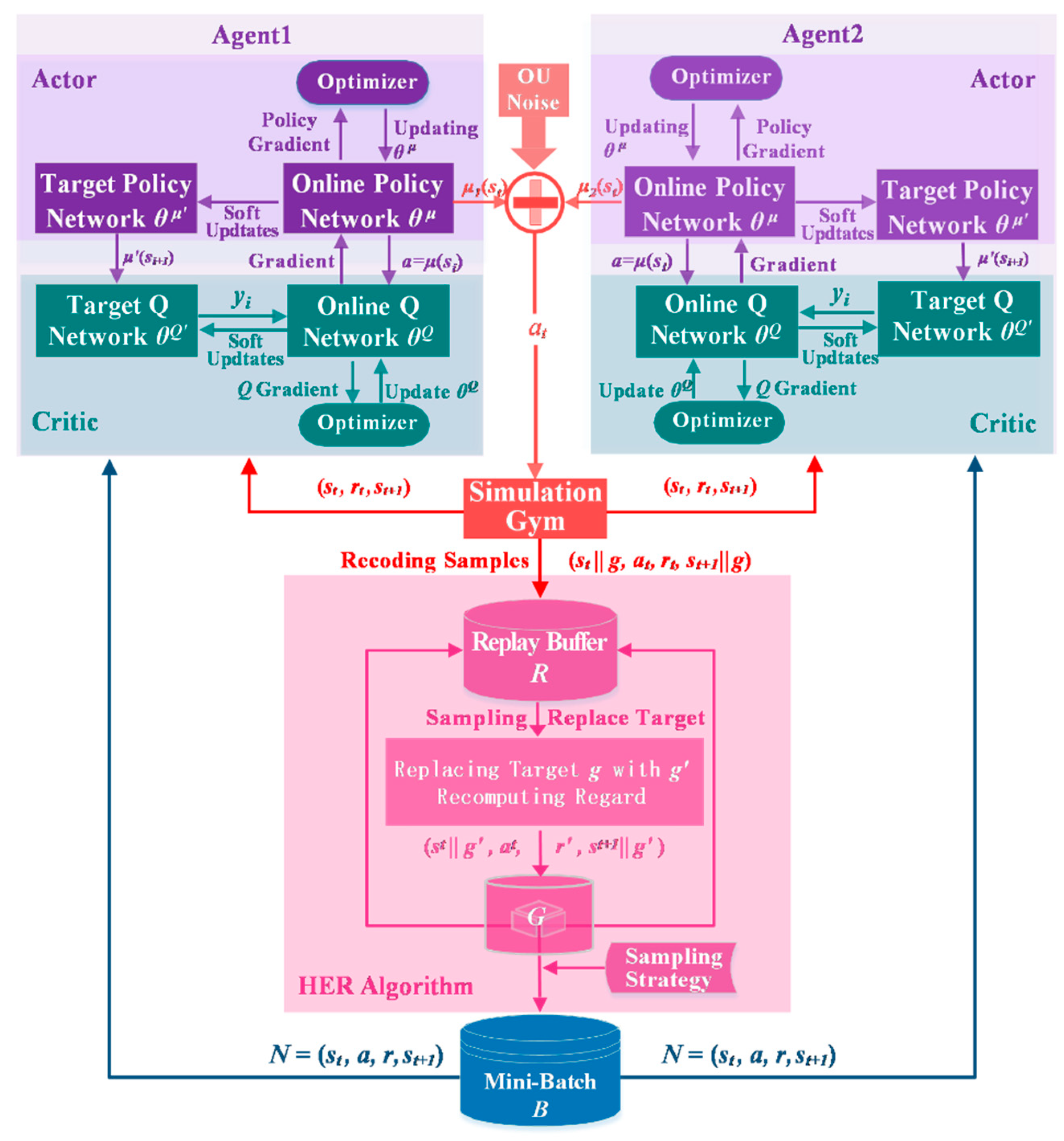
Figure 1. The block diagram for the dual-arm deep deterministic policy gradient (DADDPG) algorithm.
Applsci 11 01816 g001
Figure 2. Reach scene. (a) The left and right target positions are randomly chosen in 3D space. Control the left and right end effectors of the robot to reach the left and right targets as quickly as possible. (b) The learning curve of Reach scene—the abscissa is the number of training rounds and the ordinate is the average success rate of 10 tests.
Applsci 11 01816 g002
Figure 3. Push scene. (a) The task is to move a block placed on the table in front of the robot to the target position on the table. (b) The learning curve of Push scene—the abscissa is the number of training rounds and the ordinate is the average success rate of 10 tests.
Applsci 11 01816 g003
Figure 4. Pick up scene. (a) This task is similar to the Push scene, but the target position is in a specific area above the table. The robot needs to hold the block on the target position. (b) The learning curve of Pick up scene—the abscissa is the number of training rounds and the ordinate is the average success rate of 10 tests.
Applsci 11 01816 g004
Figure 5. Gripping pot scene. The purpose of this task is to verify the performance of the algorithm. (a) A circle protrudes from the top of the object. The robot can touch a reasonable point to grip the pot and put the pot in a specified area. (b) The learning curve begins to oscillate with a small amplitude and finally converges to the optimal solution. The abscissa is the number of training rounds and the ordinate is the average success rate of 10 tests.
Applsci 11 01816 g005
Figure 6. The algorithm transferring architecture. The simulation condition is replaced by the physical environment on the basis of the equivalence principle.
Applsci 11 01816 g006
Figure 7. The control architecture. The agent of the deep reinforcement learning algorithm is a server and sends a response to the client. The dual-arm robot is a client and requires service from the server.
Applsci 11 01816 g007
Figure 8. Renderings of Reach task of the physical robot. (a) The image obtained by the camera. The two triangles represent the current position of the fingers and the QR code used by Apriltags is pointed to by the arrow. (b) The selected target points are left and right points in the air, which are 10 cm above the QR code.
Applsci 11 01816 g008
Figure 9. The dataset of Mask-RCNN algorithm. (a) and (b) Two pictures were randomly selected to show the unlabeled images of thin rods in different positions and angles in the dataset.
Applsci 11 01816 g009
Figure 10. The identification result of Mask-RCNN algorithm. (a) Mask-RCNN can recognize the target in real-time. (b) The recognition result of the Mask-RCNN algorithm including Mask region, label, and confidence.
Applsci 11 01816 g010
Figure 11. Schematic diagram of identification result. (a) The image was taken by the camera. (b) The identification result of Mask-RCNN algorithm. (c) The result of color threshold segmentation.
Applsci 11 01816 g011
Figure 12. The ends of the thin rod in the robot’s view. The threshold of the color selected according to the pixel value of the thin green rod in the image. (a) The image obtained by the camera. (b) The recognition result of ends of the rod.
Applsci 11 01816 g012
Figure 13. (ac) The process of physical robot completes the grasping task.
Applsci 11 01816 g013
Figure 14. The problem of tilt for the thin rod. (a) Grab results in simulation environment. (b) Grasping effect of real robot. (c) The renderings in RVIZ.
Applsci 11 01816 g014
Publisher’s Note: MDPI stays neutral with regard to jurisdictional claims in published maps and institutional affiliations.