Stochastic Dosimetry Assessment of the Human RF-EMF Exposure to 3D Beamforming Antennas in indoor 5G Networks

Abstract

The deployment of near future 5G networks will introduce modifications in the population’s exposure levels to radio-frequency electromagnetic fields (RF-EMFs). The present work aimed to face the challenge of studying the exposure variability in the presence of an access point (AP) at 3.7 GHz with 64 patch elements uniform planar array antenna and 3D beamforming capability. The novelty introduced in the methodology of the exposure’s evaluation was the combining of traditional computational methods with a new approach based on stochastic dosimetry, called polynomial chaos kriging method, in order to estimate the exposure levels for 1000 different antenna beamforming patterns with low computational efforts. The simulations were evaluated considering a child model and computing the specific absorption rate (SAR) in different tissues. The analysis of the results highlighted a high exposure variability scenario depending on the beamforming patterns of the array antenna and identified the ranges of elevation and azimuth angles of the main antenna beam that may cause the highest levels of exposure.

1. Introduction

The Fifth Generation (5G) of wireless cellular networks was designed to satisfy ambitious goals such as very low latency, dramatic increase in the number of connected devices and data rates, ultra-reliable links, and high coverage. Deployment of 5G will allow the next future to be characterized by the reality of smart homes, cities, and societies, bringing new services and utilities to the whole population in an Internet of Things world [1]. Innovative technologies have been proposed in recent years and are being carried out, i.e., deployment of small-cell networks, use of massive multiple-input–multiple-output (MIMO) base station antennas, device-to-device (D2D) communication, heterogeneous networks, and three-dimensional beamforming (3DBF) techniques [2,3,4,5]. To provide enhanced broadband communications, additional spectrums have been allocated in millimeter wave (mm wave) bands between 3 and 100 GHz to make available very large channel bandwidths; however, at these high frequencies, there is the need to counterbalance the high path loss that signals experience. The use of dense micro cells’ deployments combined with antennas capable of focalizing the beam adaptively in the desired direction, by sophisticated 3DBF techniques, may effectively combat the severe path loss and reduce network interference and electromagnetic emission towards undesired directions [6,7].

In the vast multitude of studies dealing with the performance of technological solutions for 5G network deployment, some of them also deal with human exposure levels that such deployments will induce [8,9,10,11,12,13,14,15]. The authors in References [8,9] used simplified exposure models to evaluate the impact of the new mm wave frequency bands. In References [10,11,12], the authors studied the exposure levels caused by specific devices in uplink and downlink scenarios but limited only on a few configurations, and in References [13,14,15], the authors faced the variability of the exposure scenario by using ray tracing and statistical techniques [13,14,15].

It is undeniable that the introduction of new frequencies and new techniques of radio physical access will have an impact on human radio-frequency electromagnetic field (RF-EMF) exposure, and the design of new exposure assessments that take into account the heterogeneity of different link parameters (e.g., the number of array antennas, the dielectric properties of users, the 3D beamforming patterns) still represents a challenging task [16,17,18].

The present work aimed to face the challenge of studying the exposure variability in presence of this heterogeneity. In particular, the novelty of the paper is the use for the first time stochastic (metamodeling) techniques combined with the classical computation techniques (deterministic dosimetry). Stochastic dosimetry was successfully applied previously for both low- and high-frequency exposure scenarios [19,20], allowing to enormously reduce the associated computational costs by substituting an expensive computational model with a functional approximation of the original model, much faster to evaluate. In this way, starting from the results of a small number of expensive computational simulations and coupling them with surrogate models (metamodeling), it is possible to estimate the exposure in a large number of configurations and conduct statistics and sensitivity analyses [19].

The heterogeneity afforded in this study was introduced by the beamforming capability of the antenna of an access point (AP) in an indoor environment. In detail, the AP antenna was modeled by a uniform planar array (UPA) with 64 patch elements at 3.7 GHz that is inside the licensed range of frequencies below 6 GHz that the first 5G network installations will use (in Italy the range is 3.6–3.8 GHz [16]). A child model was used in the simulations to obtain the human exposure levels in terms of the specific absorption rate (SAR), as specified in the International Commission on Non-Ionizing Radiation Protection (ICNIRP) guidelines [21]. The joint use of deterministic and stochastic methods allowed us to expand the exposure assessment from a few specific beamforming patterns of the UPA antenna (as investigated in our previous study [22]) to the entire space of variability of the antenna pattern.

Details of the methodology used and a brief discussion on the surrogate models adopted are presented in Section 2. The numerical results of the simulation campaign interpolated by the use of the surrogate models are presented and analyzed by means of statistical and global sensitivity in Section 3. The results of statistical and sensitivity analyses are discussed in Section 4. Finally, the conclusions of the work are drawn in Section 5.

2. Materials and Methods

The considered exposure scenario, shown in Figure 1, was modeled to assess the exposure variability of a single user due to an AP operating at 3.7 GHz with a 64 elements UPA antenna. As detailed in Reference [22], each element of the antenna was composed by a simple patch antenna characterized by three layers. The three layers were composed by the ground layer, the patch layer modeled as PEC materials, and the substrate layer modeled by a dielectric material (dielectric properties: ${\epsilon }_{\mathrm{r}}$ = 2.25 and σ = 0.0005 S/m, data from Reference [13)]. The total dimensions of the array were 29 × 29 × 0.5 cm (right side of Figure 1), and the antenna was excited with a Gaussian signal with a total input power of 100 mW in line with the maximum allowed input power values specified in the 3rd Generation Partnership Project [23].

The human exposure levels were evaluated in terms of the SAR in the child Roberta’s model (age = 5 years old, height = 1.1 m, mass = 17.6 kg and BMI = 14.8 kg/m) from the Virtual Classroom [24] as illustrated in the left part of Figure 1. The UPA antenna was placed laterally in respect to the model head at a fixed distance of 50 cm to the central point of the head. The choices of simulating a child model, instead of an adult one, and a lateral configuration of the antenna were suggested by the findings of our previous work [22]: for fixed zero-phase shift among the different array elements (i.e., for the maximum gain in the direction perpendicular to the antenna array), the child Roberta model and the lateral configuration of the antenna showed the highest exposure levels.

To study the impact of the 3D beamforming capability of the UPA antenna, we introduced the two scan angles that regulated the beamforming direction in the H-plane (azimuth plane) and in the E-plane (elevation plane), varying respectively in the range (−50°, +50°) and (−25°, +25°) as reported in Reference [25]. As an example, Figure 2 shows the spatial antenna gain patterns for the scan angles at the extreme values of their ranges (respectively +/−50° and +/−25° for azimuth and elevation planes).

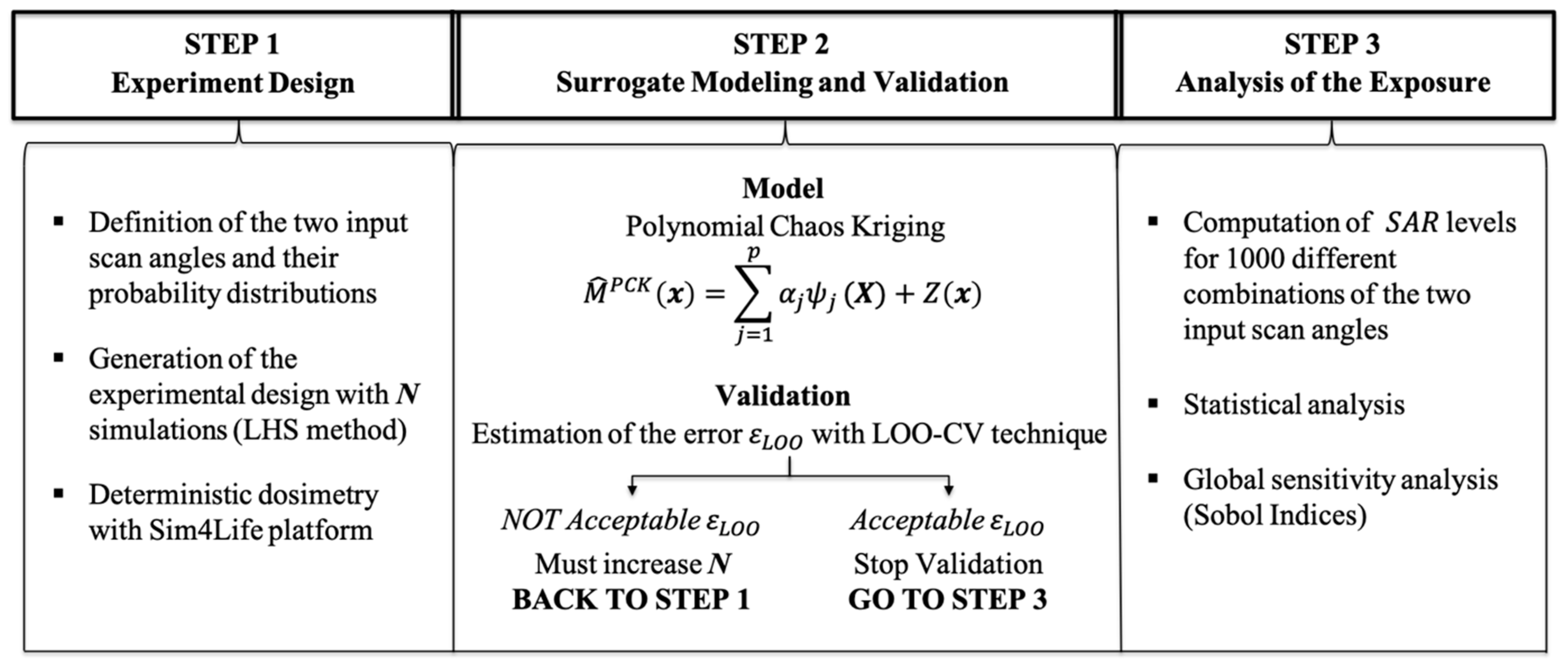
Figure 3 shows a flow chart of the methodology adopted. It combines the traditional computational methods with the stochastic dosimetry, an innovative technique that uses surrogate models to obtain the variable of interest with really low computational cost in respect to traditional computational methods. This technique was already applied either in low- or in high-frequency ranges to assess the EM exposure levels of users [19,20]. The surrogate models were obtained for the SAR values averaged on the whole body, the whole head and the whole brain and for the maximum values of SAR averaged on 10 g for specific tissues (e.g., the skin, the brain gray matter, and the cerebellum).

The three steps of the process are described in details in the sub-sections below: “Experiment Design” motivates the choice for the input setting and the deterministic simulations, “Surrogate Modeling and Validation” illustrates the construction of the surrogate models with stochastic dosimetry and their validation, “Analysis of the Exposure” highlights how the surrogate models allowed to calculate the SAR values in the tissues of interest with low computational costs, so providing a fine variability analysis of exposure assessment with 3D beamforming.

2.1. Experiment Design

The problem of the evaluation of EMF exposure can be seen as the problem of finding a computational model $M$ in the formula:

$$Y=M\left(\mathit{x}\right),$$

(1)

where $\mathit{x}$ denotes the vector of input parameters that influence the exposure scenario, and $Y$ represents the quantity of interest for the EMF exposure assessment, i.e., the averaged and the maximum SAR values in different body areas and tissues.

In this case, the input parameters are the two scan angles (Figure 1) that characterize the 3D beamforming of the UPA antenna, assuming the directions of maximum radiation in the azimuth and elevation planes uniformly distributed in the ranges (−50, +50) and (−25, +25), respectively. To generate the input coordinates, within the operational ranges, the Latin Hypercube sampling (LHS) method was applied on the input probability density functions [26].

The deterministic dosimetry simulations were then performed on the set of input parameters in Sim4Life platform (ZMT Zurich Med Tech AG, Zurich, Switzerland, www.zurichmedtech.com (accessed on 6 February 2021)), that implements the finite-difference time-domain (FDTD) solver. The computational domain of all simulations with the UPA antenna included the entire Roberta’s model discretized with a non-uniform grid with a maximum step of 0.9 mm for the human body. The Roberta’s tissues dielectric properties were chosen according to the literature [27,28], considering the antenna frequency of 3.7 GHz. At last, perfectly matched layer (PML) absorbing conditions were assumed at the domain boundaries.

To conduct the exposure assessment, the SAR was evaluated in some specific tissues. In detail, the SAR averaged on tissue mass was assessed for the whole body (${SAR}_{wb}$), the whole head ($SA{R}_{wh}$), and the whole brain ($SA{R}_{wbr}$), where the brain included the following tissues: brain grey matter, brain white matter, hippocampus, hypophysis, hypothalamus, medulla oblongata, midbrain, pineal body, pons, and thalamus. Furthermore, the $SAR$ averaged on 10 g ($SA{R}_{10g}$) was considered for the skin, the brain grey matter, and the cerebellum.

The results obtained with deterministic dosimetry were used to implement the surrogate models by the polynomial chaos kriging methods as described below.

2.2. Surrogate Modeling and Validation

A metamodeling (or surrogate modeling) technique allows for the reduction of the associated computational costs by substituting the expensive computational model $M\left(\mathit{x}\right)$ with a metamodel such as:

$$\widehat{Y}=\widehat{M}\left(\mathit{x}\right),$$

(2)

where $\widehat{Y}$ represents an analytical function with similar statistical properties as$Y$, but obtainable with significantly lower computational cost comparing to the cost of deterministic dosimetry.

In the present work, among the possible non-intrusive approaches useful to obtain surrogate models, the Polynomial Chaos Kriging technique (PC-Kriging) was chosen, which is a novel metamodeling technique that allows to combine the advantages of Kriging (Gaussian process modelling) with those of Polynomial Chaos Expansions (PCE) [29,30]. Briefly, the PC-Kriging is formed by a universal kriging model that has a trend which is modeled by a sparse set of orthogonal polynomials. Details of the individual PCE and kriging techniques plus the description of the PC-Kriging method and his validation are reported below.

2.2.1. Universal Kriging

The universal kriging, also known as Gaussian process modeling, represents a statistical interpolation method that splits the random function into a linear combination of deterministic functions, known at any point of the domain input, and a random component, the residual random function, described by a Gaussian noise depending on the input vector. The model function $\widehat{M}\left(\mathit{x}\right)$ is then described by the following equation (the apex “K” stays for “kriging”):

$${\widehat{Y}}^K={\widehat{M}}^K\left(\mathit{x}\right)={{\displaystyle \sum }}_{j=1}^p{\beta }_j{f}_j\left(\mathit{x}\right)+Z\left(\mathit{x}\right),$$

(3)

where ${{\displaystyle \sum }}_{j=1}^p{\beta }_j{f}_j\left(\mathit{x}\right)$ is a linear combination of a given functional basis $f$ with non- zero coefficients ${\beta }_j$ and represents the mean value of ${\widehat{Y}}^K$, and $Z\left(\mathit{x}\right)$ represents the stationary Gaussian process with zero mean and stationary autocovariance:

$$\mathsf{{\rm E}}\left[Z\left(\mathit{x}\right),Z\left({\mathit{x}}^{\prime }\right)\right]={\sigma }^{2}R\left(\mathit{x}-{\mathit{x}}^{\prime }, \mathit{\theta }\right),$$

(4)

Characterized by the (constant) variance ${\sigma }^2$ of the Gaussian process, and by $R$ which is its stationary autocorrelation depending on the difference between two sample points $\left(\mathit{x}-{\mathit{x}}^{\prime }\right)$ and its hyperparameters $\mathit{\theta }$. In the present work, the Matérn correlation function $R$ was used and its hyperparameters ${\mathsf{\sigma }}^2$ and $\mathit{\theta }$ were estimated by cross-validation estimation and covariance matrix adaptation-evolution strategy (CMA-ES). Further details of the autocorrelation functions properties and of the universal kriging method can be found in [31,32].

2.2.2. Polynomial Chaos Expansions

Polynomial chaos expansions (PCE) are a family of powerful stochastic techniques that provide functional approximation of a generic computational model through its spectral representation based on a suitably built basis of polynomial functions. The PCE method can be described by the following equation (the apex “PCE” stays for “polynomial chaos expansions”):

$${\widehat{Y}}^{PCE}={\widehat{M}}^{PCE}\left(\mathit{X}\right)={\displaystyle \sum }_{j=1}^p{\alpha }_j{\psi }_j\left(\mathit{X}\right),$$

(5)

where $\mathit{X}$describes the probability density function of the chosen input parameters $\mathit{x}$, $p$ is the size of the polynomial basis Ψ(X), ${\psi }_j\left(\mathit{X}\right)$ are the orthonormal polynomials belonging to Ψ(X) and ${\alpha }_j$ are the corresponding unknown coefficients to be estimated. In this work, given the uniformly distributed input parameters $\mathit{x}$, the Legendre polynomials up to the fourth order were selected as polynomial basis. Details of the different PCE techniques can be found in References [19,33].

2.2.3. Polynomial Chaos Kriging

The combination of the universal kriging with the PCE methods allows to obtain a new metamodeling technique that is more efficient than the two methods separately taken. The PC-Kriging in fact uses the regression-type PCE for capturing the global behavior of the computational model, whereas interpolation-type kriging allows to capture local variations as a function of the neighboring points of the experimental design. At the end, a more accurate metamodel is achieved by the use of the two techniques combination. The PC-Kriging method can be defined as a universal kriging model, whose mean value (trend) is formed by a set of orthonormal polynomials as in PCE technique and can be described by the following equation (the apex “PCK” stays for “polynomial chaos kriging”):

$${\widehat{Y}}^{PCK}={\widehat{M}}^{PCK}\left(\mathit{x}\right)={\displaystyle \sum }_{j=1}^p{\alpha }_j{\psi }_j\left(\mathit{X}\right)+Z\left(\mathit{x}\right),$$

(6)

where it can be noticed that the first term ${{\displaystyle \sum }}_{j=1}^p{\alpha }_j{\psi }_j\left(\mathit{X}\right)$ represents the trend of the model and is equal to the PCE solution (Equation (5)) whereas the second term$Z\left(\mathit{x}\right)$ is a calibration term as in Equation (3), represented by the stationary Gaussian process.

It is thus evident that the construction of PC-Kriging model requires two steps: (i) the determination of the orthogonal polynomials and their coefficients ${\alpha }_j$ to estimate the trend and (ii) the calibration of the Kriging model, by evaluating the variance ${\sigma }^2$ of the Gaussian process and the hyperparameters $\mathit{\theta }$ of the autocorrelation function $R$as in Equation (4).

There are various ways to jointly optimize the two parts. Among all the PC-Kriging models available, we chose the optimal PC-Kriging (OPCK) metamodel as the best one that minimizes the leave-one-out error, as detailed in the next sub-section. The OPCK estimates the optimal set of polynomials by least angle regression selection (LARS) algorithm [34], which detects a sparse set of polynomials and their corresponding coefficients in decreasing order according to their correlations to the current residual at each LARS iteration. Then, it estimates the trend of PC-Kriging model by adding each polynomial individually and calibrating for each iteration the new PC-Kriging model. The surrogate models’ solutions to PC-Kriging procedure were obtained by the software “UQLab: The Framework for Uncertainty Quantification” [35].

2.2.4. Validation of Surrogate Models

To validate the obtained surrogate models, the leave-one-out cross-validation (LOO-CV) technique, already tested on previous works [19,20], was used. The method was applied to counterbalance the needs of obtaining an acceptable error and of minimizing the number N of simulations conducted with deterministic dosimetry. In fact, starting from the initial experimental design x and its corresponding responses $Y=M\left(\mathit{x}\right)$ calculated with deterministic dosimetry, the LOO-CV error is expressed by:

$${\epsilon }_{LOO}=\frac{1}{N}\left[\frac{{{\displaystyle \sum }}_{i=1}^N{\left(M\left(x_i\right)-{\widehat{M}}_{\left(-i\right)}^{PCK}\left(x_i\right)\right)}^2}{Var\left[Y\right]}\right],$$

(7)

where $M\left(x_i\right)$ represents the model output in $x_i$ obtained with deterministic dosimetry, ${\widehat{M}}_{\left(-i\right)}^{PCK}\left(x_i\right)$ represents the output of kriging metamodel in $x_i$obtained using all the points of the experimental design $\mathit{x}$ except $x_i$, and $Var\left[Y\right]$ is the variance of the output data obtained with computational methods.

Here, the number of N = 60 simulations turned out to be adequate to guarantee an acceptable LOO-error.

2.3. Analysis of the Exposure

After the validation of the PC-Kriging, we built the surrogate models of the SAR quantities of interest. The average SAR (namely, for the whole body, the whole head and the whole brain) and the maximum $SA{R}_{10g}$ in specific tissues (e.g., the skin, the brain gray matter, and the cerebellum) were estimated on 1000 different combinations of the two input angles in the azimuth and elevation planes. To better characterize the exposure levels, the data were statistically processed, calculating the Quartile Dispersion Coefficient (QDC) for each SAR distribution as:

$$QDC=\frac{Q_3-Q_1}{Q_3+Q_1},$$

(8)

where $Q_1$ and $Q_3$ are respectively the first and third quartiles of the distribution.

To identify the scan angles ranges that might cause the highest exposure levels, an analysis of the ranges inducing $SAR$ values higher that the 70% of their maximum value was conducted for each SAR distribution.

Finally, in order to evaluate which angle, between azimuth and elevation, mostly influences the exposure levels, a global sensitivity analysis was conducted using the Sobol variance-based method [36]. This method decomposes the system output variance as the sum of the partial variances as contributions due to the fact of each input parameter; the Sobol indices are calculated as the ratios between the partial variances and the total variance of the system output. The Sobol indices reported in the tables are normalized with respect to the sum of all the Sobol indices under consideration.

3. Numerical Results

Here, we report the numerical results obtained following the illustrated methodology (Figure 3).

First of all, the validation LOO-CV errors (Equation (7)) have been computed for the obtained surrogate models based on the results of N = 60 simulations, i.e., 60 different combinations of beamforming scan angles. The error values are reported in

Table 1. LOO-Error values of the surrogate models for tissue average SAR in the whole body, whole head, and whole brain and for $SA{R}_{10g}$ in skin, brain grey matter, and cerebellum.

	Whole Body	Whole Head	Whole Brain	Skin	Brain Grey Matter	Cerebellum
LOO Error	0.31%	0.27%	0.94%	2.85%	2.06%	5.70%

. They ranged from a minimum of 0.27%, computed for the average SAR in the whole head, to a maximum of 5.70% for the $SA{R}_{10g}$ in the cerebellum, thus proving sufficiently low error values to validate the model.

Once the surrogate models were validated, they were used to estimate the exposure levels in terms of both average SAR and maximum $SA{R}_{10g}$ for 1000 different combinations of azimuth and elevation angles of the main radiation beam.

Figure 4 and Figure 5 and

Table 2. The QDC values, the percentage of SAR values higher than the 70% of the maximum values, and the corresponding ranges of elevation and azimuth angles for whole body, for whole head, and for whole brain.

	Whole Body	Whole Head	Whole Brain
QDC	71.7%	73.5%	74.8%
% > 0.7 maximum	7.2%	4.7%	3.3%
Range H-plane	From −7° to 7°	From −8° to 6°	From −6° to 7°
Range E-plane	From −22° to 7°	From −10° to 7°	From 1° to 7°

refer to the average SAR results on the whole body on the whole head and on the whole brain, while Figure 6 and Figure 7 and

Table 3. The QDC values, the percentage of SAR_10g higher than the 70% of the maximum values and the variation range extremes of the two input parameters for the skin, for the brain grey matter and for the cerebellum.

	Skin	Brain Grey Matter	Cerebellum
QDC	67.4%	74.6%	76.0%
% > 0.7 maximum	3.3%	4.2%	2.8%
Range H-plane	From −5° to 5°	From −10° to 6°	From −5° to 5°
Range E-plane	From −11° to 4°	From −5° to 10°	From −4° to 8°

refer to maximum $SA{R}_{10g}$ results on the skin, on the brain grey matter and on the cerebellum. The exposure levels are estimated for a total input power of the UPA antenna equal to 100 mW.

Minimum, maximum, and median values and the first and the third quartiles of the $SAR$ distributions are shown as boxplots in Figure 4. We can see that (i) the highest SAR values were obtained for the whole head, with a maximum of 8.35 mW/kg, a median of 0.42 mW/kg and a mean value of 1.23 mW/kg; (ii) the SAR values for the whole brain were around half of those computed for the head (maximum 4.17 mW/kg, median 0.16 mW/kg and mean 0.48 mW/kg), and (iii) the lowest values were obtained for the whole body with a maximum of 1.75 mW/kg, a median of 0.12 mW/kg, and a mean value of 0.32 mW/kg. The highest SAR values obtained for the whole head and for the whole brain could be explained considering the position of the UPA antenna with respect to the model. In fact, the head was with higher probability hit by the boresight beam of the UPA antenna (that is the beam with direction orthogonal to the array and providing the highest power) and this did not happen for the lower part of the body. Furthermore, we noticed that for all the three SAR distributions mean and median values were close, while the maximum values differed by about one order of magnitude w.r.t. them, meaning that the distributions concentrated in a small range around their mean values as the boxplots show.

Figure 5 shows, for each surrogate model, a map of the SAR on the plane of the 1000 combinations of azimuth angles, in the range (−50°, +50°), and elevation angles, in the range (−25°, +25°) (first row of Figure 5), and two graphs, extracted from the corresponding map of SAR, one varying the azimuth angles of the beam, fixed the elevation angle to 0° (second row of Figure 5), and the other one varying the elevation angles, fixed the azimuth angle to 0° (third row of Figure 5). The plots highlight the high variability of the exposure levels in all the three SAR distributions depending on the beamforming patterns in the H- and E-planes. To give a quantitative idea of this variability Table 2 reports the QDC values, the percentages of values greater than 70% of the maximum value and the ranges of elevation and azimuth angles corresponding to these highest exposure levels.

The table shows that QDC values vary from a maximum of 75% in the whole brain to a minimum of 72% in the whole body and the percentage of values higher that the 70% of the maximum values are really low, 7.2% for the whole-body, 4.7% for the whole head and only 3.3% for the whole brain. Looking at the SAR maps in Figure 5 and the “Range H-plane” values in Table 2, we realize that, for all the three SAR distributions, the highest exposure levels corresponded to beamforming patterns with the beam focused on the azimuth plane in a symmetric narrow range (about 14°) approximately 0°, that is just the alignment direction between the antenna and Roberta’s body in the H-plane. On the other hand, in the E-plane, things change, and the area of higher exposure varies depending on the part of the body. The highest SAR levels in the whole body distribute on the range (−22°, 7°), covering the shoulder area of the model. Instead, the highest SAR levels for the whole head and for the whole brain concentrate in narrower ranges, respectively, (−10°, 7°) and (0.6°, 7°), and out of these narrow ranges the main antenna beam does not intercept these body areas.

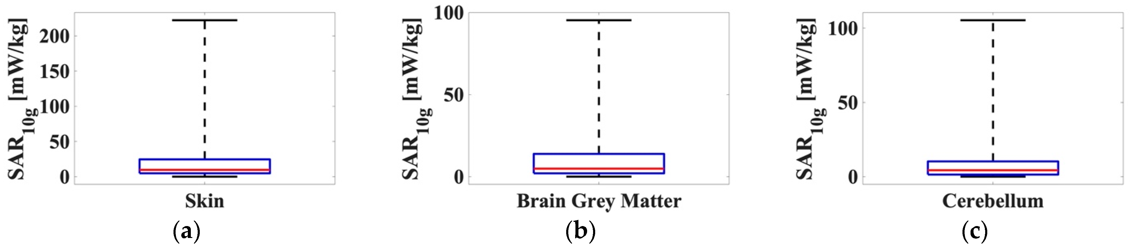
The same analysis was also conducted for the maximum SAR averaged on 10 g for the skin, the brain grey matter, and the cerebellum. The boxplot of the 1000 SAR_10g values obtained are reported in Figure 6.

In this case, the highest SAR_10g values were obtained for the skin tissue, with a maximum value of 222.23 mW/kg, a median value equal to 9.71 mW/kg, and a mean value equal to 26.80 mW/kg. The SAR_10g obtained for the brain grey matter and cerebellum were close to each other with values that were around half of the values obtained for the skin (precisely, max = 95.24 mW/kg, median = 4.89 mW/kg, mean = 13.30 mW/kg for the brain grey matter and max = 105.32 mW/kg, median = 4.37 mW/kg mean = 10.86 mW/kg for the cerebellum).

Figure 7 reports, analogously to Figure 5, a map of the values on the plane of the 1000 combinations of azimuth angles, in the range (−50°, +50°), and elevation angles in the range (−25°, +25°), and two graphs, one varying the azimuth angles of the beam, fixed the elevation angle to 0°, and the other one varying the elevation angles fixed the azimuth angle to 0°.

The results of the deeper statistical analysis, i.e., the QDC values, the percentage of SAR_10g values higher than 70% of the maximum and the ranges of elevation and azimuth angles corresponding to these highest exposure levels are reported in Table 3.

In addition, for $SA{R}_{10g}$, the QDC values remained high (from a maximum value of 76% for the cerebellum to a minimum of 67.4% for the skin), whereas the percentage of highest values is really low. For the skin this percentage was only 3.3%, the brain grey matter was 4.2%, and the cerebellum only 2.8%. It can be noticed again that the highest $SA{R}_{10g}$ levels corresponded to beams concentrated in a symmetrical small range around 0° in the azimuth plane for the skin and the cerebellum, while for the brain grey matter the range was slightly unbalanced (−10°, 6°). A slightly larger variability on the exposure levels was measured varying the beam direction on the elevation plane, but the amplitude of ranges remained small, varying from 12° to 15°.

Finally, a global sensitivity analysis based on Sobol indices was conducted for all the SAR distributions here considered, and the results are reported in Figure 8. The normalized Sobol indices for the azimuth angles showed high values, from 70% and 80%, definitely higher than the values measured for the elevation angles. Moreover, the Sobol indices for the elevation angles showed non-negligible values, especially for the brain tissues (i.e., the whole brain, the brain gray matter, and the cerebellum), where are around 30%. This is a quite interesting result, that highlights how the azimuth angles of the main beam of antenna arrays with 3D beamforming capability have a predominant role on the exposure levels, even if also the elevation angles have a non-negligible impact on exposure levels especially for the brain area. These considerations obviously derive from the relative position between the UPA antenna and the model and from the 3D shape of the human body model.

4. Discussion

In the present paper, an innovative approach that combined universal kriging with polynomial chaos expansions technique (called polynomial chaos kriging PCK method) was used in the electromagnetic dosimetry framework in order to assess for the first time the exposure levels of a single user in a future indoor 5G scenario that deploys an antenna array with beamforming capability. This method represents a further option to the approaches previously used in stochastic dosimetry [19,20], which typically focused on the use of surrogate models to describe the variability of exposure in uncertain conditions.

Although there are not yet at present commercial solutions to 5G indoor access points with 3D adaptive beamforming, the roll-out of small cells will be a key point for success of 5G networks as reported in Reference [16]. The massive deployment of low-power AP will be primarily in the frequency band of 3.5–3.7 GHz, and in the future, in higher frequency bands above the 24 GHz in order to bring higher data capacities and higher data rate transmission. In this work, we modeled a 64 patch element UPA antenna at 3.7 GHz with 3D beamforming capability for a total input power of 100 mW, in line with the maximum allowed input power for indoor hotspot reported in the 3rd Generation Partnership Project [23], i.e., 250 mW. The distance between the UPA antenna and the model head was simulated at 50 cm to evaluate the highest SAR levels. Greater distances between the AP and the human body will lead to lower SAR levels.

The aim of the work was to validate the stochastic dosimetry methodology to obtain a complete description of the exposure levels for any beamforming patterns of the UPA antenna in terms of SAR distributions with an affordable computational effort respect to deterministic simulation methods; this aim was reached by identifying the effectiveness of the PCK method.

Even if the distance between the antenna and the human subject was closer compared to a possible real implementation, the estimated exposure levels still led to low levels of SAR that respect the EMF exposure limitations. In fact, all the highest observed values for the SAR averaged on the whole body, the whole head, and the whole brain, and for the SAR_10g on tissues were significantly below the reference levels that ICNIRP guidelines introduce as basic restrictions for general public exposure, i.e., 0.08 W/kg for the whole body average SAR and 2 W/kg for the local head and torso $SA{R}_{10g}$[21]. These results are also in line with those of previous studies regarding 5G networks deployments, which estimated the exposure levels in indoor environments and highlighted that the ICNIRP guidelines will be well respected [13,14]. Furthermore, the analysis conducted on the QDC values showed QDC values always higher than 67% for all the six examined SAR distributions. This means that, although low, the exposure levels change consistently as a function of the azimuth and elevation angles of the antenna beam that describes the space of variability of the 3D beamforming of the UPA antenna. This was an expected result, as 3D beamforming techniques inherently focus the radiation in narrow beams to increase the gain in the target direction and not everywhere [5,6,7] thus introducing a high variability on the induced SAR in the child model tissues.

This consideration is reinforced by the analysis of the SAR values higher than the 70% of their maximum values, that showed how the highest values of the SAR concentrate in small ranges of the elevation and azimuth angles. The analysis highlighted also how only the beamforming patterns directed primarily towards the model area led to high SAR levels, whereas main antenna beams directed in other directions cause a rapidly decrease of SAR values.

Moreover, the global sensitivity analysis showed that the azimuth angle, which describes the beamforming variation in the H-plane, has a predominant role in the induced SAR exposure levels in all the six distributions examined, though also the elevation angle in the E-plane is relevant, even if with a lower impact, especially for brain tissue. The variation of the elevation angle can indeed influence the power of the radiated wave towards the area where these tissues are morphologically placed. These considerations highlighted that it is crucial to consider both the azimuth and the elevation angles to obtain surrogate models able to reliably describe the exposure level due to indoor 5G AP deploying antenna arrays with 3D beamforming capability.

5. Conclusions

In conclusion, stochastic dosimetry has been shown to be suitable to face the variability of the EMF body exposure levels in next generation networks, that will be characterized by inherent growing uncertainty, heterogeneity and complexity. In this perspective, there is the need of validating numerical estimation methods with affordable computational efforts, passing from realistic to surrogate models. In particular, the PCK method revealed to be an efficient tool for surrogate modelling dealing with the exposure levels caused by 3D beamforming of array antennas that 5G APs will introduce. The analysis conducted with the proposed method highlighted the impact of the elevation and azimuth angles of the main radiation beams on SAR distributions. Although in the future it will be very interesting to carry out environmental measurements of the exposure levels caused by the physical AP devices that will actually be implemented in 5G network, from the quantitative results that this analysis provided we can confirm that the radiation focusing capability that 3D beamforming implements will lead to low levels of SAR, significantly below the ICNIRP guidelines for general public exposure.