A Set of Active Disturbance Rejection Controllers Based on Integrator Plus Dead-Time Models ^†

Abstract

The paper develops and investigates a novel set of constrained-output robust controllers with selectable response smoothing degree designed for an integrator-plus-dead-time (IPDT) plant model. The input-output response of the IPDT system is internally approximated by several time-delayed, possibly higher-order plant models of increasing complexity. Since they all contain a single integrator, the presented approach can be considered as a generalization of active disturbance rejection control (ADRC). Due to the input/output model used, the controller commissioning can be based on a simplified process modeling, similar to the one proposed by Ziegler and Nichols. This allows it to be compared with several alternative controllers commonly used in practice. Its main advantage is simplicity, since it uses only two identified process parameters, even when dealing with more complex systems with distributed parameters. The proposed set of controllers with increasing complexity includes the stabilizing proportional (P), proportional-derivative (PD), or proportional-derivative-acceleration (PDA) controllers. These controllers can be complemented by extended state observers (ESO) for the reconstruction of all required state variables and non-measurable input disturbances, which also cover imperfections of a simplified plant modeling. A holistic performance evaluation on a laboratory heat transfer plant shows interesting results from the point of view of the optimal least sensitive solution with smooth input and output.

1. Introduction

Efficient control is important in many fields, especially in power generation, transportation, agriculture, industry, and households. In this paper, the focus is on fast and efficient temperature control of a complex and uncertain temperature process. The dynamics studied are similar to many other physical processes. For example, diesel engine control, air–fuel ratio control in gasoline engines, control of DC-DC converters, continuous stirred tank reactors (CSTR), or micro-electro-mechanical systems (MEMS) [1,2,3,4,5,6,7,8,9]), to name a few.

Automatic control algorithms with different possible design paradigms are used to realize fast, robust and smooth transients. Active Disturbance Rejection Control (ADRC) represents one of the most popular approaches to design robust controllers for complex nonlinear systems that require simplified approach [10,11,12]. Robust control, proportional-integrative-derivative (PID) control [13,14,15,16], or model-predictive-control (MPC) [17,18,19] are other well-known and commonly used alternatives.

This work extends the ADRC-based approach presented in the conference paper [20]${}^{†}$. The latter deals with the simplest plant approximations in the state-space design, extended by disturbance-observer-based integral action introduced to reconstruct and compensate input disturbances. At the same time, the considered structures have been used to illustrate the core ideas behind the commonly used, but usually not sufficiently clarified, ADRC structures. Since with each simplification we get closer to oversimplification, the method should be presented clearly enough and should be compatible to other alternative control designs [21], especially those tending to higher-order controllers [22] with a more effective noise attenuation.

In principle, ADRC uses the state observer and the controller designed in the state-space. The ADRC is based on the extended state observer (ESO). In addition to the reconstruction of the state of the considered system, it also reconstructs the overall input disturbance, which is the result of external disturbances and model inaccuracies. The work of [23] has already brought the first such solutions using the approaches used today in ADRC and disturbance-observer based control. Unlike PID controllers, which do not consider the exact reconstruction of disturbances and pay for it with the emergence of windup-effect, resistance to control signal limitations is one of the basic advantages of systems with reconstruction of input or output disturbances.

Use of the simplest integrative models represents another dominant feature of ADRC. Simplified modeling of systems simplifies their identification as well as the design and implementation of controllers. Modeling inaccuracies are taken into account in the reconstructed disturbance and compensated by the increased robustness of the obtained solutions.

ADRC was introduced by J. Han [24] and further developed by Z. Gao [25,26] and his collaborators extensively. However, the basic advantages of the simplifications on which the ADRC is based have been used by a number of other authors, not to mention only Ziegler and Nichols and their method for experimental setup of controllers [27].

This paper focuses on aspects related to time delays that are always present, while showing the possibilities of using higher-order controllers. These are present mainly due to fractional-order PID controllers [28,29,30,31], which aim to introduce additional “tuning knobs” that can be used to adjust the controller to benefit the controlled processes. The higher-order controllers can also reduce the sensitivity to the modeling uncertainties of controlled systems, as shown in [32]. Starting with the dead-time compensation in ESO proposed already in [33], this paper develops new dead-time compensating ADRC structures based on higher-order stabilizing controllers not yet included it an overview of the current state of the literature [12].

The paper is organized as follows. Section 1 presents several possible interpretations of the two-parameter Integral Plus Dead Time (IPDT) plant models for designing higher-order Active Disturbance Rejection Control (ADRC) based control algorithms with dead-time compensation. Section 2 discusses the optimal tuning of the proportional (P), proportional-derivative (PD), or proportional-derivative-accelerative (PDA) controllers used to stabilize the IPDT models. Section 3 discusses the Extended State Observer (ESO), for reconstructing lumped disturbances and uncertainties affecting the considered (generally higher-order) integrative plant models. Section 4 then deals with an illustrative experiment with description and results of near minimum-time and, at the same time sufficiently smooth temperature control of a laboratory thermal plant. After discussing the obtained results in Section 5, the paper is concluded by Section 6.

1.1. More Realistic and Consistent Plant Modeling

The main difference of this work compared to the original paper [20] is related to the use of more realistic and at the same time more consistent plant models. They are based on the Integral Plus Dead Time (IPDT) model with the estimated gain $K_m$ and dead time $T_m$

$$S\left(s\right)=\frac{Y\left(s\right)}{U\left(s\right)}=\frac{K_m}{s}{e}^{-T_{m}s}$$

(1)

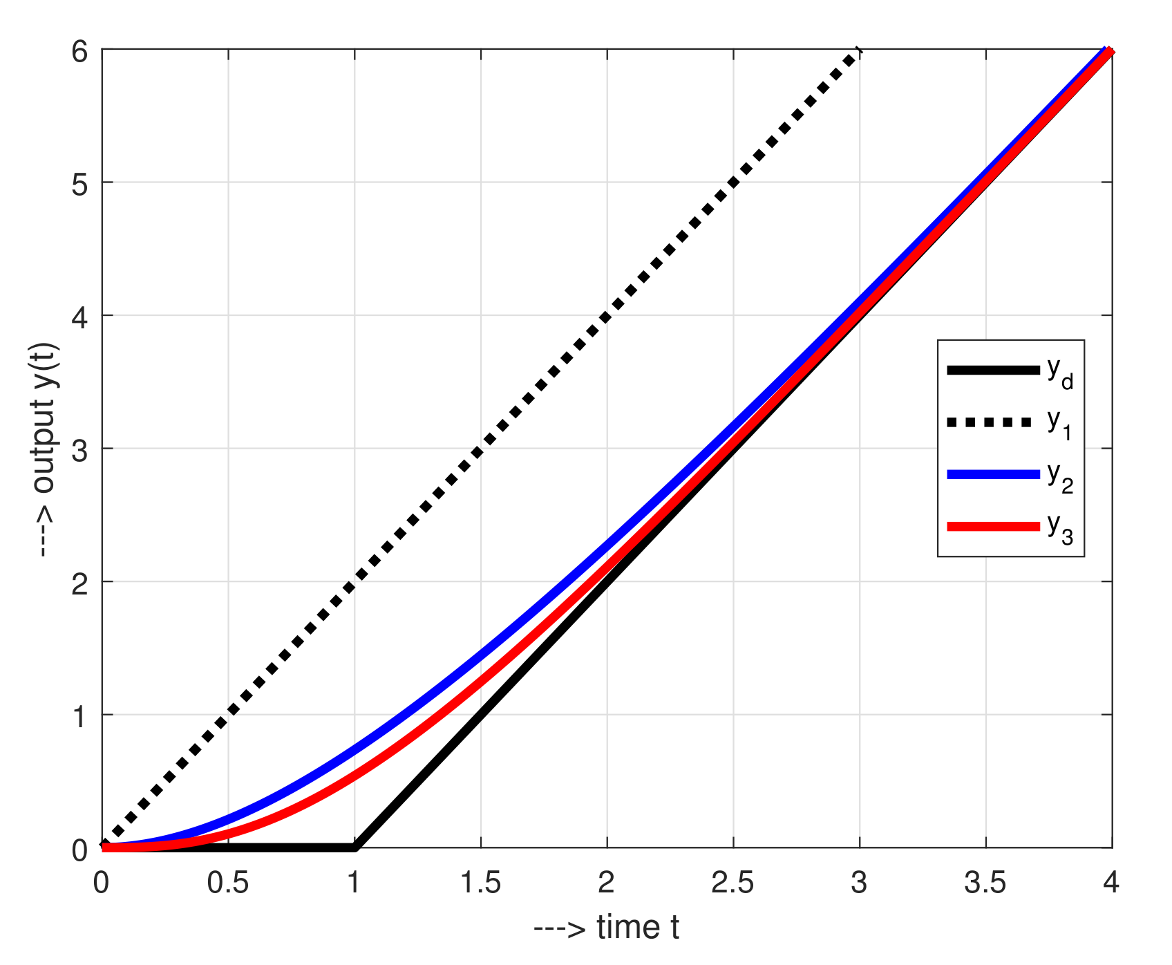
This model represents the most commonly used plant approximation in PID control design. In order to use the state-space approach, the dead time was initially avoided [34,35]. For this reason, the first approximations were dead-time free plants. To increase the accuracy of an nth order model, only a single parameter-an $n-1$ tuple time constant was added for the delay approximation. In this way, a set of nth order transfer functions $S_n\left(s\right),n=1,2,\dots$

$$\begin{array}{c}{S}_1\left(s\right)={\displaystyle \frac{Y\left(s\right)}{U\left(s\right)}}={\displaystyle \frac{K_s}{s}}\hfill \\ S_2\left(s\right)={\displaystyle \frac{Y\left(s\right)}{U\left(s\right)}}={\displaystyle \frac{K_s}{s(T_{1}s+1)}}\hfill \\ S_3\left(s\right)={\displaystyle \frac{Y\left(s\right)}{U\left(s\right)}}={\displaystyle \frac{K_s}{s{(T_{2}s+1)}^2}}\hfill \\ ⋮\hfill \end{array}$$

(2)

were established, characterized by the corresponding unit step responses (Figure 1)

$$\begin{array}{c}{y}_1\left(t\right)=K_{s}t\hfill \\ y_2\left(t\right)=K_s\left[t-T_1\left(1-e^{-t/T_1}\right)\right]\hfill \\ y_3\left(t\right)=K_s\left[t\left(1+e^{-t/T_2}\right)-2T_2\left(1-e^{-t/T_2}\right)\right]\hfill \\ ⋮\hfill \end{array}$$

(3)

By choosing $T_i=T_m/i,i=n-1,n=2,3,\dots$, the introduction of $S_2\left(s\right)$, or $S_3\left(s\right)$ for $y_2\left(t\right)$ and $y_3\left(t\right)$ allows to keep the same asymptote of the IPDT system. In this chain of approximations, $y_1\left(t\right)$ was an exception that was inconsistent with the measured IPDT step response and its higher-order dead-time-free approximations. In order to remove this inconsistency and also to avoid an increase in sensitivity to the measurement noise that occurs due to the increased state-space controller orders n, in this work the plant models are considered in the following form

$$\begin{array}{c}{S}_n\left(s\right)={\displaystyle \frac{Y\left(s\right)}{U\left(s\right)}}={\displaystyle \frac{K_s{e}^{-{\overline{T}}_{d}s}}{s{(T_{i}s+1)}^i}}\hfill \\ \mathrm{for}n=1;{\overline{T}}_d=T_m;\mathrm{i}.\mathrm{e}.,\tau =1;T_i=0;\hfill \\ \mathrm{for}n=2,3,\dots ;i=n-1;{\overline{T}}_d=\tau T_m;T_i=T_m{\displaystyle \frac{1-\tau }{i}};\tau \in (0,1)\hfill \end{array}$$

(4)

Here, $\tau$ denotes the part of the identified dead-time $T_m$ that is modeled by the transport delay ${\overline{T}}_d$, and the rest is considered as the contribution of the i time constants $T_i$. It should be remember, however, that since such approximations allow the reconstruction of higher-order output derivatives, they can also be useful for the control of loops with pure dead time by higher-order controllers. Therefore, similar to fractional-order control, we introduced “two additional tuning knobs”, n and $\tau$, which can be used to optimize the loop dynamics. In this way we extend the range of ADRC modifications [12] that are suitable for time-delayed systems.

1.2. Two Sets of Active Disturbance Rejection Controllers without and with Dead-Time Compensation

Based on the main ADRC paradigms, in [20], the sequence of plant models (2) was used to design a set of controllers denoted as ADRC${}_n,n=1,2,\dots$. The controllers have shown interesting properties and indicated a possible connection to solutions known as higher order ADRC. In this paper, we show how the mentioned set of controllers can be easily transformed into a new set of controllers denoted as ADRC${}_n\left(T_d\right)$. These fully respect the dead time $T_d$ of the IPDT model under consideration. The consequences of such a transformation are tested experimentally.

Ideally, the model parameters $T_m$ and $K_m$ should be equal to the integral plant parameters $T_d$ and $K_s$. Since the dead time $T_d$ considered in the controller tuning may differ from the dead time $T_m$ obtained from the plant identification, we need to distinguish these two values. As presented by Ziegler and Nichols [27], and discussed in numerous publications [36,37], such plant approximations can be widely applied. Here, the approximations are based on drawing a tangent line through the inflection point of the plant step response (process reaction curve). Such approaches can widely be considered also in the ADRC domain (see e.g., [5]).

2. Tuning of P, PD and PDA Controllers for IPDT Plant Considering the Dead-Time Values

As a result of the dead-time present in the loop, the state-space controllers and observer design may not be carried out in the same way as proposed in [20]. Instead of the pole assignment method, the controller parameters will be derived by the multiple-real-dominant-pole (MRDP) method [38]. When using $S_1\left(s\right)$ and the P controller gain $K_P$, the design may be based on the requirement of a double real dominant pole [39]$s_o$ of the closed loop characteristic quasi-polynomial

$$A\left(s\right)=s{e}^{T_{d}s}+K_s{K}_P$$

(5)

It may obviously be expressed in the form

$$A\left(s\right)={(s-s_o)}^2{A}_{red}\left(s\right)$$

(6)

where $A_{red}\left(s\right)$ represents a quasi-polynomial of an decreased order. Since $s_o$ yields both $A\left(s_o\right)=0$ and $dA\left(s\right)/ds=2(s-s_o)A_{red}\left(s\right)+d{A}_{red}\left(s\right)/ds=0$, i.e.,

$${\left\{A\left(s\right);\frac{d}{ds}A\left(s\right)\right\}}_{s=s_o}=\mathbf{0}$$

(7)

from

$$\frac{d}{ds}A\left(s\right)=e^{T_{d}s}+s{T}_d{e}^{T_{d}s}=0$$

(8)

follow the double dominant pole $s_o$

$$s_o=-1/T_d$$

(9)

and the corresponding dominant loop time constant $T_o=-1/s_o=T_d$. A substitution into (5) yields

$$K_{Po}={\displaystyle \frac{1}{K_s{T}_d{e}^1}}$$

(10)

For the IPDT plant, the MRDP method also allows to calculate an optimal tuning of the proportional-derivative (PD) controller

$$R_s\left(s\right)={\displaystyle \frac{U\left(s\right)}{E\left(s\right)}}=K_P+K_{D}s;E\left(s\right)=W\left(s\right)-Y\left(s\right)$$

(11)

When wishing to avoid control signal kicks after the step changes of the setpoint reference signal $w\left(t\right)$, the control signal has to be calculated according to

$$u\left(t\right)=K_P(w-y)-K_D\dot{y}$$

(12)

The corresponding closed loop quasi-polynomial is

$$A\left(s\right)=s{e}^{T_{d}s}+K_s{K}_{D}s+K_s{K}_P$$

(13)

In order to find the optimal parameters yielding the fastest possible transients not yet exhibiting oscillations, it has to include triple real dominant pole $s_o$, when $A\left(s\right)={(s-s_o)}^3{A}_{red}\left(s\right)$ and $s_o$ has to fulfill equations

$${\left\{A\left(s\right);\frac{d}{ds}A\left(s\right);\frac{d^2}{d{s}^2}A\left(s\right)\right\}}_{s=s_o}=\mathbf{0}$$

(14)

From

$$\frac{d^2}{d{s}^2}A\left(s\right)=[s{T}_d^2+2T_d]e^{T_{d}s}=0$$

(15)

the triple dominant pole and the corresponding dominant loop time constant follow as

$$s_o=-2/T_d;T_o=-1/s_o=T_d/2$$

(16)

A substitution into the first equations then yields

$$K_{Po}={\displaystyle \frac{4}{K_s{T}_d{e}^2}};K_{Do}={\displaystyle \frac{1}{K_s{e}^2}}$$

(17)

Similarly, it is possible to continue with finding ideal stabilizing proportional-derivative-accelerative (PDA) controller with the gains $K_P,K_{D1},K_{D2}$

$$R_s\left(s\right)=K_P+K_{D1}s+K_{D2}{s}^2$$

(18)

when

$$u\left(t\right)=K_P(w-y)-K_{D1}\dot{y}-K_{D2}\ddot{y}$$

(19)

From the characteristic quasi-polynomial

$$A\left(s\right)=s{e}^{T_{d}s}+K_s{K}_{D2}{s}^2+K_s{K}_{D1}s+K_s{K}_P$$

(20)

yields the condition of quadruple real dominant pole $s_o$ in $A\left(s\right)={(s-s_o)}^4{A}_{red}\left(s\right)$

$${\left\{A\left(s\right);\frac{d}{ds}A\left(s\right);\frac{d^2}{d{s}^2}A\left(s\right);\frac{d^3}{d{s}^3}A\left(s\right)\right\}}_{s=s_o}=\mathbf{0}$$

(21)

with

$$\frac{d^3}{d{s}^3}A\left(s\right)=[s{T}_d^3+3T_d^2]e^{T_{d}s}=0$$

(22)

optimal values

$$s_o=-3/T_d;T_o=-1/s_o=T_d/3$$

(23)

and

$$K_{Po}={\displaystyle \frac{27}{2K_s{T}_d{e}^3}};K_{D1o}={\displaystyle \frac{5}{K_s{e}^3}};K_{D2o}={\displaystyle \frac{T_d}{2K_s{e}^3}}$$

(24)

The benefits of higher-order controllers are evident from the integral of absolute error (IAE) values of the unit setpoint step responses. In the case of monotonic step responses, they may be calculated from the Laplace transform as integral of error (IE)

$$\begin{array}{c}IAE=IE=\underset{s\to 0}{lim}s{\displaystyle \frac{1}{s}}\left[1-{\displaystyle \frac{R_s\left(s\right)S\left(s\right)}{1+R_s\left(s\right)S\left(s\right)}}\right]{\displaystyle \frac{1}{s}}=\underset{s\to 0}{lim}E\left(s\right)\hfill \end{array}$$

(25)

whereby the first $1/s$ corresponds to integration and the last to the setpoint unit step. When introducing normed dimensionless $iae$ values, their decreasing values demonstrate ideal benefits of the more complex controllers

$$\begin{array}{c}iae=IAE/T_d\hfill \\ ia{e}_P=2.718;ia{e}_{PD}=1.847;ia{e}_{PDA}=1.488\hfill \end{array}$$

(26)

However, when using higher order controllers based on the plant models (4), two problems appear:

• Models $S_1\left(s\right)$ will preferably be used for P controller design-the use of PD controllers would require to obtain or generate output derivative $\dot{y}$; for PDA controllers both derivatives $\dot{y}$ and $\ddot{y}$ have to be acquired, which either requires additional sensors, or filters/observers, and to take into account their parameters;
• Models $S_2\left(s\right)$ may directly be combined with the PD controller and models $S_3\left(s\right)$ with PDA controller; however, it yet is necessary to take into account impact of the time constants $T_i$. The simplest possibility is to reduce models (4) to an equivalent IPDT system by considering the “half-rule” [13] with an equivalent dead-time $T_e=T_1/2$. In case of the transfer function $S_2\left(s\right)$ it increases the loop deadtime $T_m$ to

  $$T_d={\overline{T}}_d+\frac{T_1}{2}=T_m(\tau +\frac{1-\tau }{2})=T_m\frac{1+\tau }{2}$$

  (27)
  However, experiments show that such equivalence is sufficiently precised just for $T_1<<T_m$. For longer $T_1$, approximately for $T_1>T_m/2$, it may be more appropriate to work with “average residence time” based equivalence [14,40], when

  $$T_d={\overline{T}}_d+T_1=T_m$$

  (28)
  Similar estimates of $T_d$ may be derived for $S_3\left(s\right)$.

Before addressing impact of these simplifications on the controller tuning in details, let us look at the problem of disturbance reconstruction and compensation.

3. Extended State Observer

In real time control, deviations always appear between the behavior of real plants and their models. Such differences may be explained by considering impact of some equivalent disturbances acting at the plant output or input. Use of output disturbances was typical for the internal model control (IMC). Since it lead to several problems in control of integrative and unstable plants (as unobservable output disturbances of integrative plants, see e.g., [21,41], or unbounded disturbances of unstable ones [42]), it is more appropriate to deal with input disturbances d, as in ADRC. There, all the plant-model discrepancies and external actions are merged into an eqwuivalent input disturbances. By merging the unknown disturbance with the plant state to be reconstructed by an Extended State Observer (ESO), it is possible to construct controller which does not need to identify the internal plant feedback as in traditional linear and nonlinear controller design. Such lumped disturbances and uncertainties are represented by an additional state without identifying a specific input responsible for its changes. In order to keep the system model simple, effects of particular state variables on input are not considered, even in situations, when they may be supposed to be known.

For tracking all the $n+1$ state variables (including the input disturbance d) of real nth order systems, it is required to tune $n+1$ ESO coefficients.

3.1. ADRC1 Contoller Design

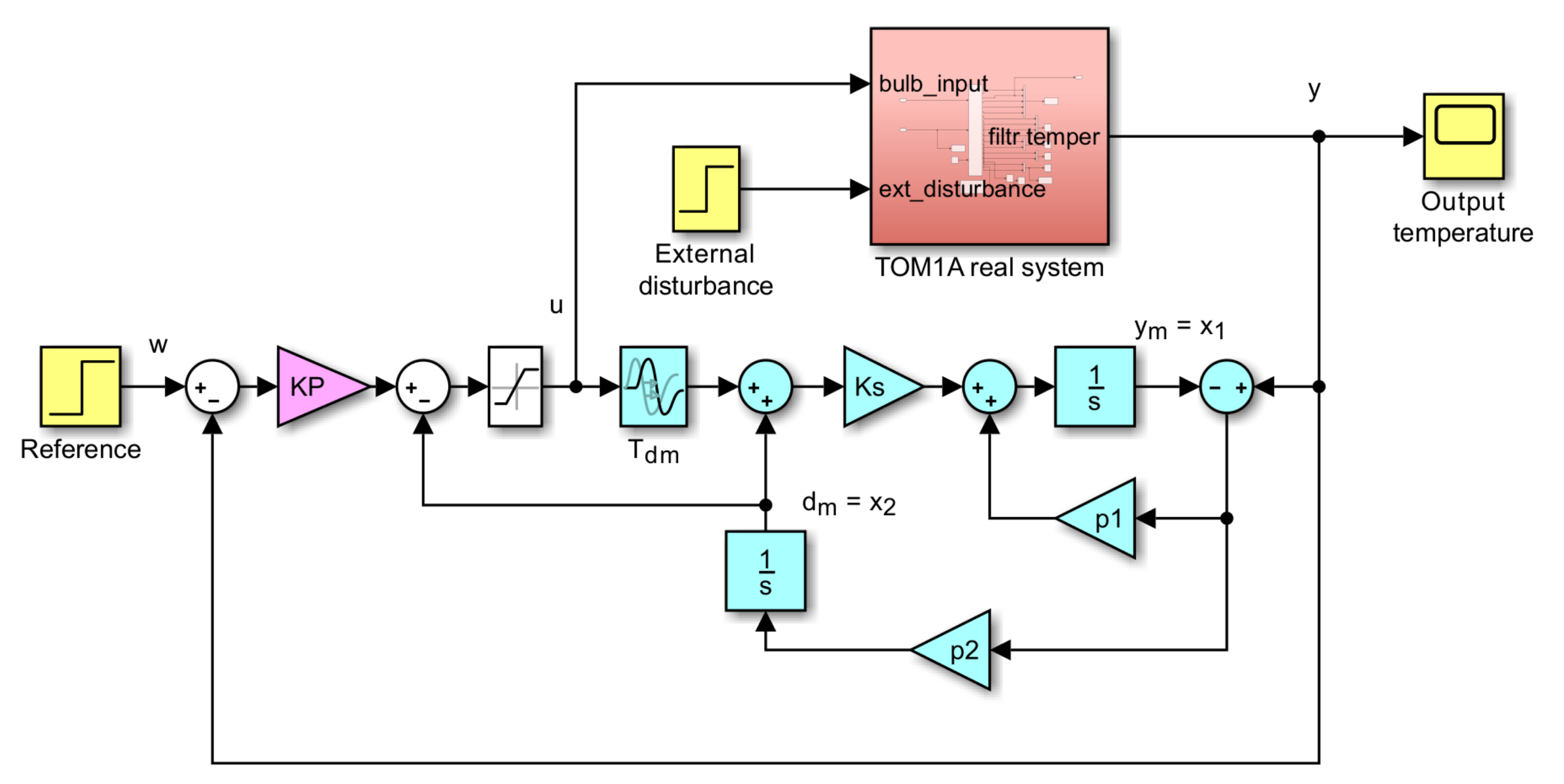
ESO is a dynamic system into which the control signal and the difference between the outputs of the controlled system and its model enter. Most simple case with process model $S_1\left(s\right)$, the extended state observer above results in the following expressions (Figure 2) yields the state equations (the model output $y_m$ which is given by the state $x_1$ will be denoted as $\overline{y}$; disturbance $d_m=\overline{d}$ corresponds to $x_2$)

$$\begin{array}{c}{\dot{x}}_1=(x_2+u(t-T_d))K_s+p_1(y-\overline{y});\overline{y}=x_1\hfill \\ {\dot{x}}_2=0+p_2(y-\overline{y})\hfill \end{array}$$

(29)

The expression (29) can be written as:

$$\begin{array}{l}\dot{\mathbf{x}}=\left[\begin{array}{cc}-p_1& K_s\\ -p_2& 0\end{array}\right]\mathbf{x}+\left[\begin{array}{c}{K}_s\\ 0\end{array}\right]u(t-T_d)+\left[\begin{array}{c}{p}_1\\ p_2\end{array}\right]y;\\ \overline{y}=\left[10\right]\mathbf{x};\overline{d}=\left[01\right]\mathbf{x}\end{array}$$

(30)

For equally delayed plant and model outputs y and $\overline{y}$ ($T_m={\overline{T}}_d$), the extended state observer dynamics described as:

$$det\left(s\mathbf{I}-\overline{\mathbf{A}}\right)=\left[\begin{array}{cc}s+p_1& -K_s\\ p_2& s\end{array}\right]=s(s+p_1)+K_s{p}_2$$

(31)

does not explicitly depend on $T_d$. By selecting the pair of poles at $s=-1/T_c$, the calculated ESO parameters are chosen according to

$$p_1={\displaystyle \frac{2}{T_c}};p_2={\displaystyle \frac{1}{T_c^2{K}_s}}$$

(32)

With respect to the time constant of the stabilizing control (9), we may expect as a reasonable choice $T_c\approx T_d$. The disturbance rejection, especially in the steady-state, can be achieved by subtracting $\overline{d}$ from the inner proportional controller. When taking into account the limitations of the controller output, the solution results in ADRC${}_1$ controller (see Figure 2). Of course, with respect to possible uncertainty in approximating real loop dead-time $T_d$ by the chosen model dead-time ${\overline{T}}_d$, $T_c$ may not be chosen too short.

3.2. ADRC2 Controller Design

When considering integrative model $S_2\left(s\right)$ with a time constant $T_1$, ESO (Figure 3) may be described as

$$\begin{array}{c}{\dot{x}}_1=x_2+p_1(y-\overline{y})\hfill \\ {\dot{x}}_2=-x_2/T_1+K_s(x_3+u(t-\overline{T_d}))/T_1+p_2(y-\overline{y})\hfill \\ {\dot{x}}_3=0+p_3(y-\overline{y})\hfill \\ \overline{y}=x_1\hfill \end{array}$$

(33)

This model offers both the input disturbance estimate $\overline{d}=x_3$ and the output derivative estimate $\dot{\overline{y}}\approx x_2$ useful for the PD controller (12) (alternatively, it might be calculated from the first row in (33).

When neglecting differences in delays of the plant and model, ESO dynamics may be described by

$$\begin{array}{l}\dot{\mathbf{x}}=\left[\begin{array}{ccc}-p_1& 1& 0\\ -p_2& -1/T_1& K_s/T_1\\ -p_3& 0& 0\end{array}\right]\mathbf{x}+\\ +\left[\begin{array}{c}0\\ K_s/T_1\\ 0\end{array}\right]u(t-{\overline{T}}_d)+\left[\begin{array}{c}{p}_1\\ p_2\\ p_3\end{array}\right]y;\\ \overline{y}=\left[100\right]\mathbf{x};\dot{\overline{y}}\approx \left[010\right]\mathbf{x};\overline{d}=\left[001\right]\mathbf{x}\end{array}$$

(34)

Its dynamics is then characterized by

$$\begin{array}{c}det\left(s\mathbf{I}-\overline{\mathbf{A}}\right)=\left[\begin{array}{ccc}s+p_1& -1& 0\\ p_2& s+1/T_1& -K_s/T_1\\ p_3& 0& s\end{array}\right]=\hfill \\ =s^3+s^2(p_1+1/T_1)+s(p_1/T_1+p_2)+p_3{K}_s/T_1\hfill \end{array}$$

(35)

By choosing three poles at $s=-1/T_c$, the ESO parameters become

$$\begin{array}{c}{p}_1={\displaystyle \frac{3}{T_c}}-{\displaystyle \frac{1}{T_1}};p_2={\displaystyle \frac{3}{T_c^2}}-{\displaystyle \frac{p_1}{T_1}};p_3={\displaystyle \frac{T_1}{K_s{T}_c^3}}\hfill \end{array}$$

(36)

With respect to accelerated transients with the closed loop time constant (16), one may expect as a reasonable choice $T_c\approx T_d/2$. Thereby, according to the “half-rule” [13], dead-time $T_d$ of the IPDT plant should equal to the modified loop delay $T_d={\overline{T}}_d+T_1/2$. However, experiments show that such equivalence is appropriate just for $T_1<<T_m$. For longer $T_1>T_m/2$, it is more appropriate to work with “average residence time” equivalence yielding $T_d\approx {\overline{T}}_d+T_1$. Moreover, since “half rule” holds only for significantly small $T_1$, we do not make large error by choosing $T_d={\overline{T}}_d+T_1$ in all cases.

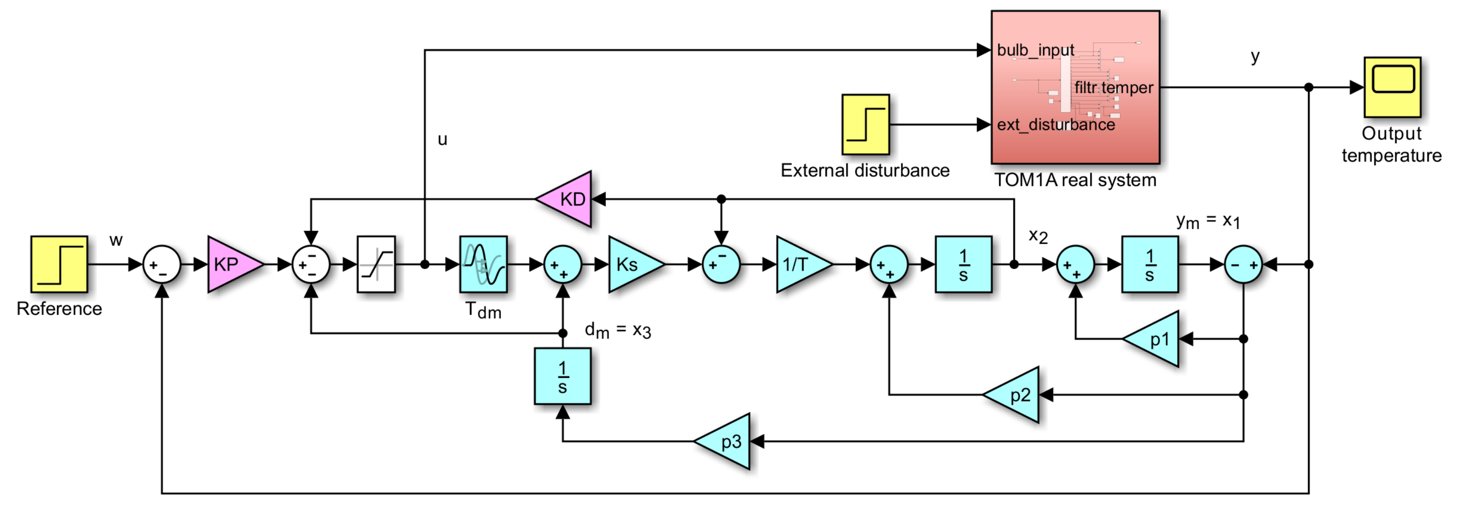
3.3. ADRC3 Controller Design

For the system

$$\begin{array}{l}\dot{\mathbf{x}}=\left[\begin{array}{cccc}-p_1& 1& 0& 0\\ -p_2& 0& 1& 0\\ -p_3& -1/T_2^2& -2/T_2& K_s/T_2^2\\ -p_4& 0& 0& 0\end{array}\right]\mathbf{x}+\\ +\left[\begin{array}{c}0\\ 0\\ K_s/T_2^2\\ 0\end{array}\right]u(t-{\overline{T}}_d)+\left[\begin{array}{c}{p}_1\\ p_2\\ p_3\\ p_4\end{array}\right]y;\\ \left[\begin{array}{c}\overline{y}\\ \dot{\overline{y}}\\ \ddot{\overline{y}}\\ \overline{d}\end{array}\right]\approx \left[\begin{array}{c}1000\\ 0100\\ 0010\\ 0001\end{array}\right]\mathbf{x}\end{array}$$

(37)

and selection of four poles at $s=-1/T_c$ and equally delayed outputs we get the observer parameters

$$\begin{array}{c}{p}_1={\displaystyle \frac{4}{T_c}}-{\displaystyle \frac{2}{T_2}};p_2={\displaystyle \frac{6}{T_c^2}}-{\displaystyle \frac{2p_1{T}_2+1}{T_2^2}}\hfill \\ p_3={\displaystyle \frac{4}{T_c^3}}-{\displaystyle \frac{p_1+2p_2{T}_2}{T_2^2}};p_4={\displaystyle \frac{T_2^2}{K_s{T}_c^4}}\hfill \end{array}$$

(38)

Here, the ESO gives the variables $\dot{\overline{y}}$, $\ddot{\overline{y}}$ and $\overline{d}$. The are used both in the PDA controller (18) and for input disturbances rejection. With respect to the speed of transients with the closed loop time constant (23), one may expect as a reasonable choice $T_c\approx T_d/3$.

Remark 1.

In the controllers it is possible to use either the plant (y), or the observer’s output ($\overline{y}$), whereby the second possibility significantly decreases impact of the measurement noise [20].

4. Real-Time Experiments and Analysis

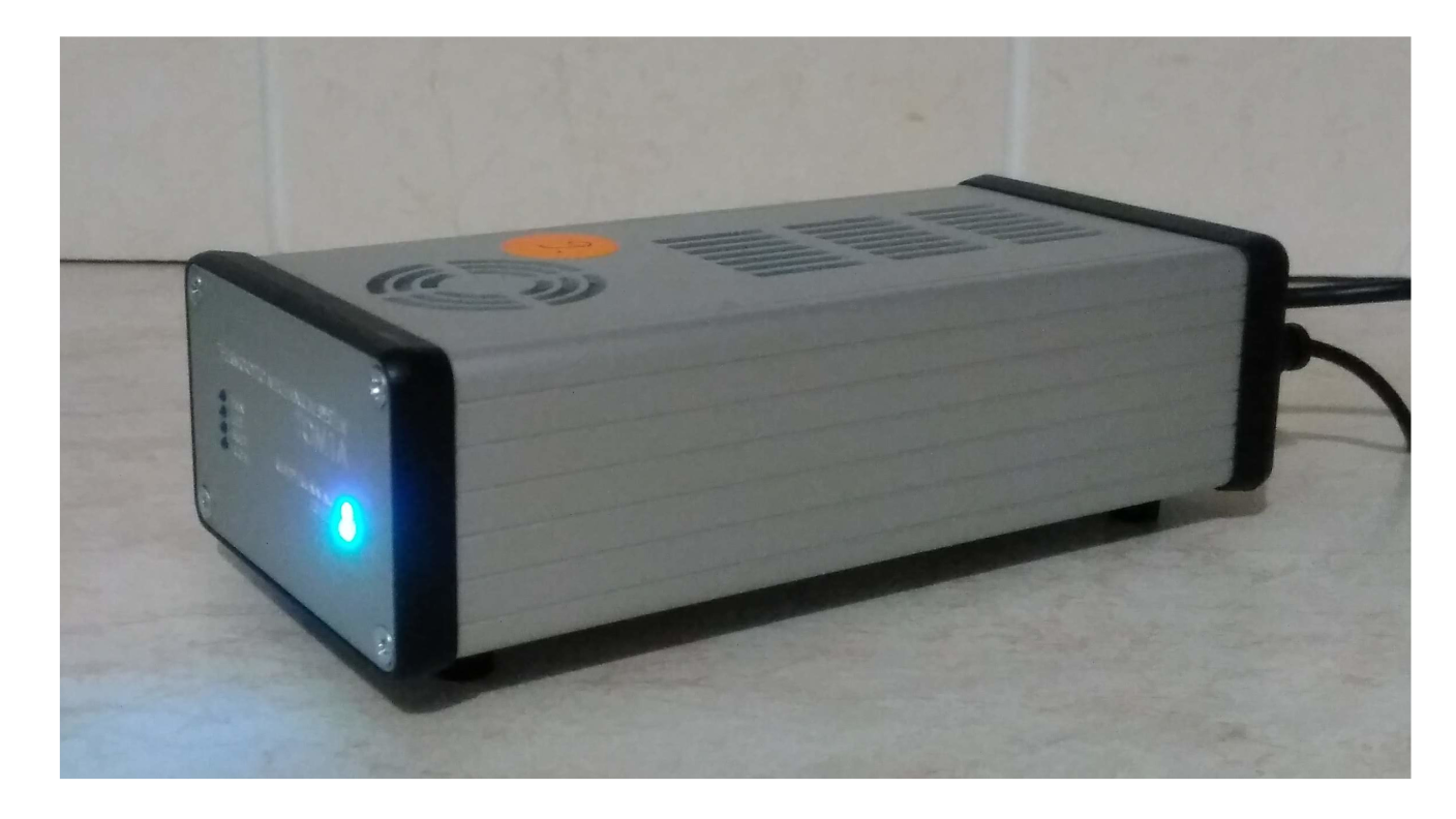
The proposed ADRC${}_n$ (i.e., ADRC${}_n\left(0\right)$) and ADRC${}_n\left({\overline{T}}_d\right)$ solutions were tested on thermo-opto-mechanical laboratory plant TOM1A (Figure 4) [43,44]. A detailed physical analysis of the thermal channel may be found in [45]. The analytical description of this channel includes several nonlinear relationships: nonlinear dependence of the required power on the input voltage, nonlinear dependence of the resistance of the lamp filament on temperature, or nonlinear Stefan-Boltzmann law describing the power radiated from a black body depending on its temperature. Similarly, cooling of the temperature sensor by means of the fan rotation provides other analytically difficult aspects to describe. With respect to two dominant heat transfer modes by radiation and conducting, or with regard to the division of the whole device into a sensor and the remaining construction, the plant model should have at least two poles, but the relative order one. The optimization of the closed loop control would therefore require a special pole assignment controller [46]. Identification experiments necessary for specifying parameters of the corresponding modes may take several hours, during which all possible disturbances must be eliminated. Furthermore, they lead to bad-conditioned mathematical solutions.

4.1. Simplified Plant Models

On the other hand, a very rough asymptotic IPDT approximation with a few seconds of necessary experiments (see e.g., [47]) yields parameters

$$K_m=0.1;T_m=0.3 \mathrm{s}$$

(39)

Based on this result, several models (4) may be proposed. With the sake of simplicity, the average-residence-time equivalence (28) has been considered, when:

$$\begin{array}{c}{S}_1\left(s\right):K_s=0.1;T_d=0.3 \mathrm{s}\hfill \\ S_2\left(s\right)={\displaystyle \frac{K_s{e}^{T_{d}s}}{s(T_{1}s+1)}};T_1=T_d(1-\tau );\tau \in (0,1)\hfill \\ S_3\left(s\right)={\displaystyle \frac{K_s{e}^{T_{d}s}}{s{(T_{2}s+1)}^2}};T_2=T_d{\displaystyle \frac{1-\tau }{2}};\tau \in (0,1)\hfill \end{array}$$

(40)

whereby three different values of $\tau$ have been considered

$${\tau }_1=0.75;{\tau }_2=0.5;{\tau }_3=0.25$$

(41)

The actual controllers were implemented in Matlab-Simulink scheme which were connected to the actual plant via USB port. The sampling time $T_s=0.02$ s was chosen close to the lower hardware limits. All the time constants used fulfill the requirement ${\tau }_i>>T_s$ important for the quasi-continuous controller implementation.

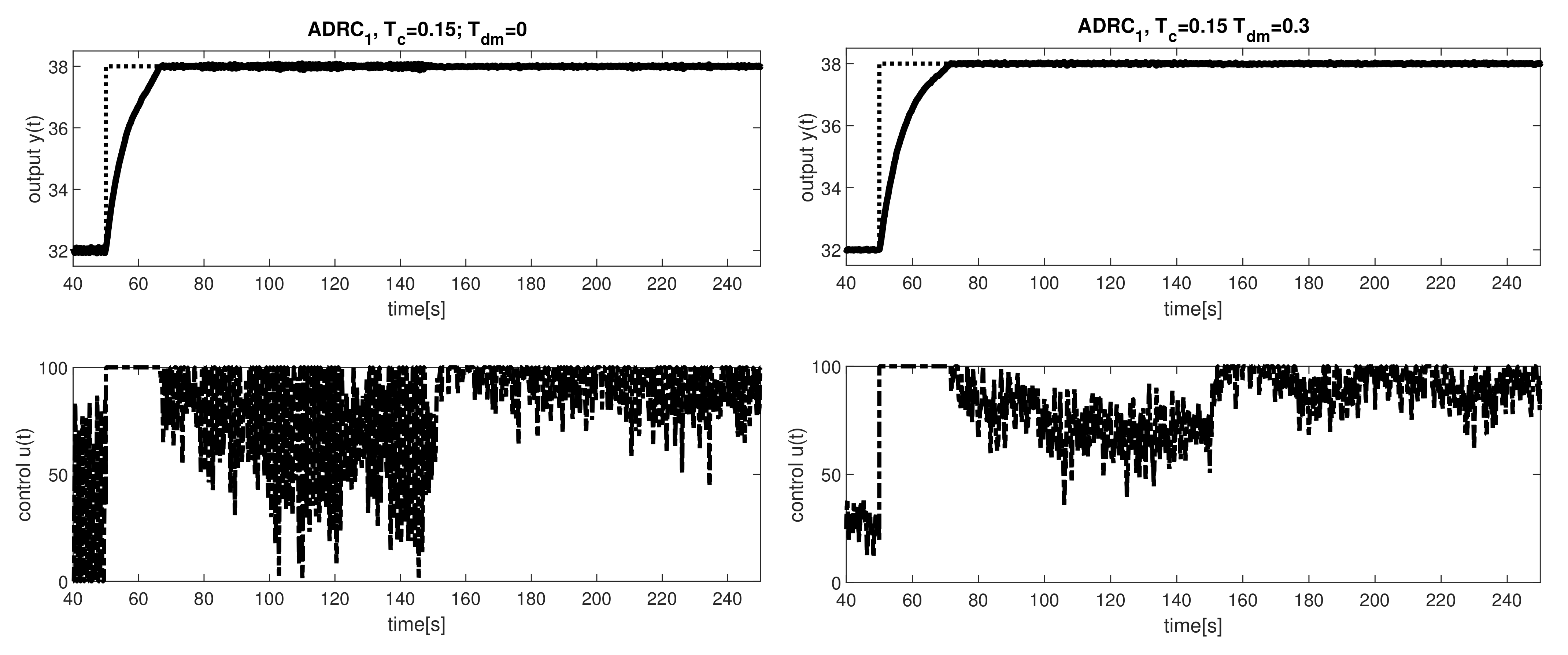
4.2. Process Transients

During the experiment, the reference was first set to $y_0=32$ °C to reach the initial steady state. Then, the reference step change to to $w=38$ °C was initiated at $t=50$ s. At $t=150$ s, the plant input disturbance was introduced by changing the fan control value from $u_{fan}=5$ to $u_{fan}=15$.

Property 1

(Basic feature of ADRC output setpoint responses). Samples of transients in Figure 5 show similar behavior as, for example, analyzed in [48]. However, the output setpoint responses clearly differ from the setpoint responses achieved by traditional PID control by the pure termination of transients after reaching the setpoint value. As shown by [49] on the example of the PI controller, in order to reduce the control signal after reaching the setpoint from the upper limit to a steady-state value, an over-regulation (negative values of the control error) must appear in the process. This basic overshooting of PI and PID control after reaching setpoint value can only be eliminated by using 2-DoF controllers, but this slows down the setpoint responses.

4.3. Time- and Shape-Related Performance Measures

Performance evaluation has two main tasks: Evaluate the robustness of the system in terms of the control structure used and its settings and evaluate the impact of noise. Control robustness has traditionally been evaluated on the basis of frequency criteria and sensitivity functions. If we realize that its primary goal was to avoid oscillating and too slow solutions, the experimental evaluation in the time domain must be able to capture these two moments.

In order to evaluate the responses in the presence of noise, the appropriate performance indicators should be used. The most basic indicator is the calculation of the total variation ($TV$) [13]. This is mostly used for evaluating excessive control effort, but in $TV$ it is mixed together with the meaningful control activities. Thus, when wishing to get not just some data proportional to the excessive activities, but a performance measure offering a clear mathematical and physical interpretation, such a more detailed performance evaluation can be achieved by calculating the deviations from monotony. This can be calculated as total variation of a variable exceeding the expected meaningful variable changes. So, for example, for a monotonic output transition between $y_0$ and $y_{\infty }$ (as after the setpoint change in Figure 5) it may be derived as

$$\begin{array}{c}T{V}_0\left(y\right)=\sum _i\left|y_{i+1}-y_i\right|-\left|y_{\infty }-y_0\right|\hfill \end{array}$$

(42)

The input signal for a monotonic output change of the considered first order system [50] consists of two distinct monotonic intervals (signal increasing and decreasing and vice versa). Such a shape will be denoted as one-pulse (1P). In measuring deviations from 1P, we have to apply the previous evaluation from monotony twice. For example, for $u\left(t\right)$ with initial and final values $u_0$ and $u_{\infty }$ and monotonic intervals separated by an extreme value (or an interval at a saturation, as in Figure 5) $u_m\notin (u_0,u_{\infty })$

$$T{V}_1\left(u\right)=\sum _i\left|u_{i+1}-u_i\right|-\left|2u_m-u_{\infty }-u_0\right|$$

(43)

In this figure, $T{V}_1\left(u\right)$ corresponding to $T_c=0.15$ will be significantly higher than for $T_c=0.6$. The algorithm for the calculation of the performance indicators may be found in [20]. Performance measures corresponding to transients in Figure 5 are in Figure 6.

4.4. Evaluation of ADRC1

As the first moment of the evaluation of transients in Figure 5, it should be noted that the action variable u is, under the strong influence of noise, a large part of the transients and also in the vicinity of steady states at the limit. Nevertheless, there is no permanent error in the system as when using PID controllers with anti-windup [51].

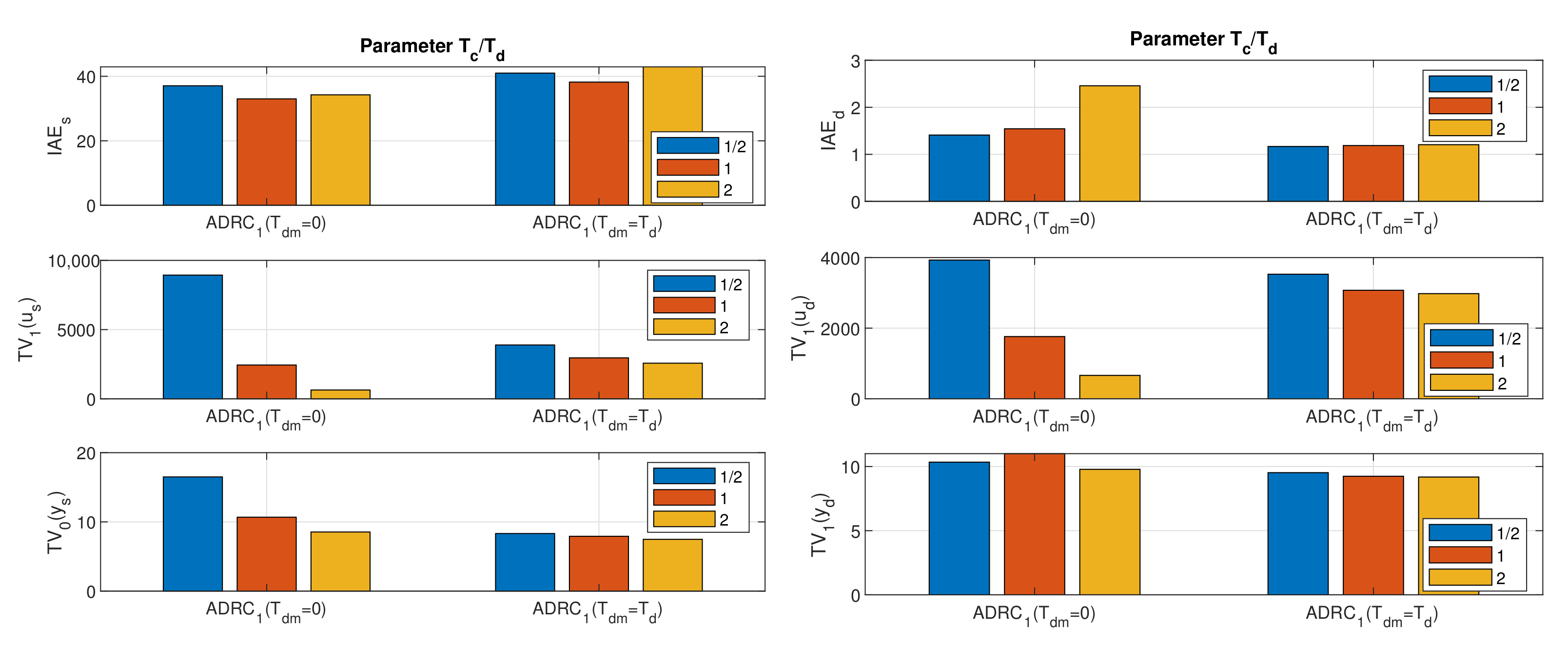
Performance measures in Figure 6 quantify the visual experience available from Figure 5. The most significant deviations correspond to the ADRC${}_1$ not considering $T_d$ (${\overline{T}}_d=0$) which occur with a relatively fast disturbance observer tuned for $T_c=T_d/2=0.15$. For this tuning, the output wobbling around required states leads already to a slight increase of $IA{E}_s$. However, it is much more visible by significantly increased $T{V}_1\left(y_s\right)$ and $T{V}_1\left(u_s\right)$ values.

Other found differences show slightly higher values of $IA{E}_s$ of controllers with the disturbance observer input delayed by ${\overline{T}}_d=T_d$ compared to similar values of the first type of controllers with ${\overline{T}}_d=0$. This result could lead to the hypothesis that the ${\overline{T}}_{dm}$ value used is too large, so it already degrades performance. However, for the disturbance steps, lower $IA{E}_d$ values of the controller with ${\overline{T}}_d=T_d$ contradict this hypothesis.

The comparison can be finished by concluding that the controllers with ${\overline{T}}_d=T_d$ depend on the tuning parameter $T_c$ determining the speed of the disturbance observer less than controllers setting with $T_c$ also $K_P$. This result can also be interpreted as an increased sensitivity (reduced robustness) of the first set of controllers at $T_c=T_d/2$, signalized by increased shape deviations at the input and output. For the second set of controllers, the sensitivity is roughly uniform and without significant peaks.

Remark 2

(An ambiguous benefit of dead-time compensation). Experiments have shown that by compensating for ${\overline{T}}_d=T_{dm}$ at the ESO input, as suggested in [33], the performance of disturbance step responses improves, but worsens for setpoint step responses. For these, a more effective way to reduce the excessive input and output increments is to increase the $T_c$ value. This raises the question of whether it would not be better to compensate only part of the identified dead-time in ESO. In the next we will solve the given problem by including some time-constant delays as part of the identified dead-time. In this way, we also obtain additional state variables suitable for the use of higher-order controllers.

4.5. Evaluation of ADRC2

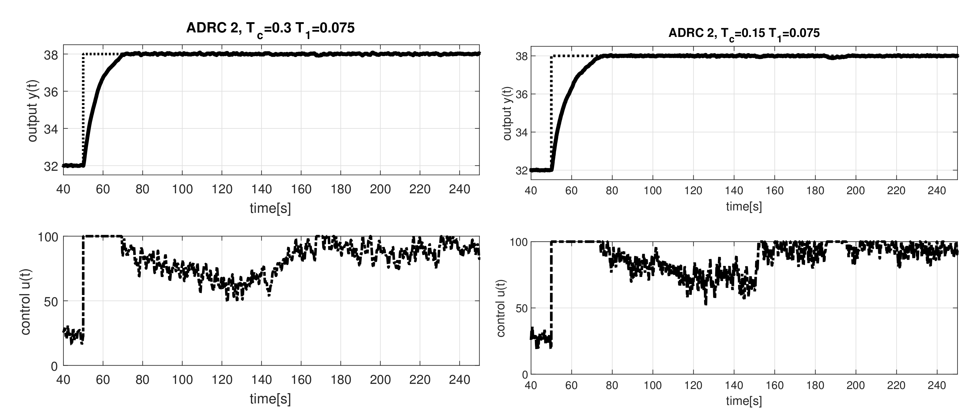
In evaluation of ADRC${}_2\left({\overline{T}}_d\right)$ controllers with the ESO delay ${\overline{T}}_d=T_d$ we will focus on choice of the ESO parameters $T_c=T_d$ and $T_c=T_d/2$ and analyze, how these values can be combined with the tuning parameter $T_1$.

The results corresponding to responses in Figure 7 show (see Figure 8) that acceleration of transients by decreasing $T_c$ increases the effect of noise. The excessive control effort is, however, generally lover than in case of ADRC${}_1$ control.

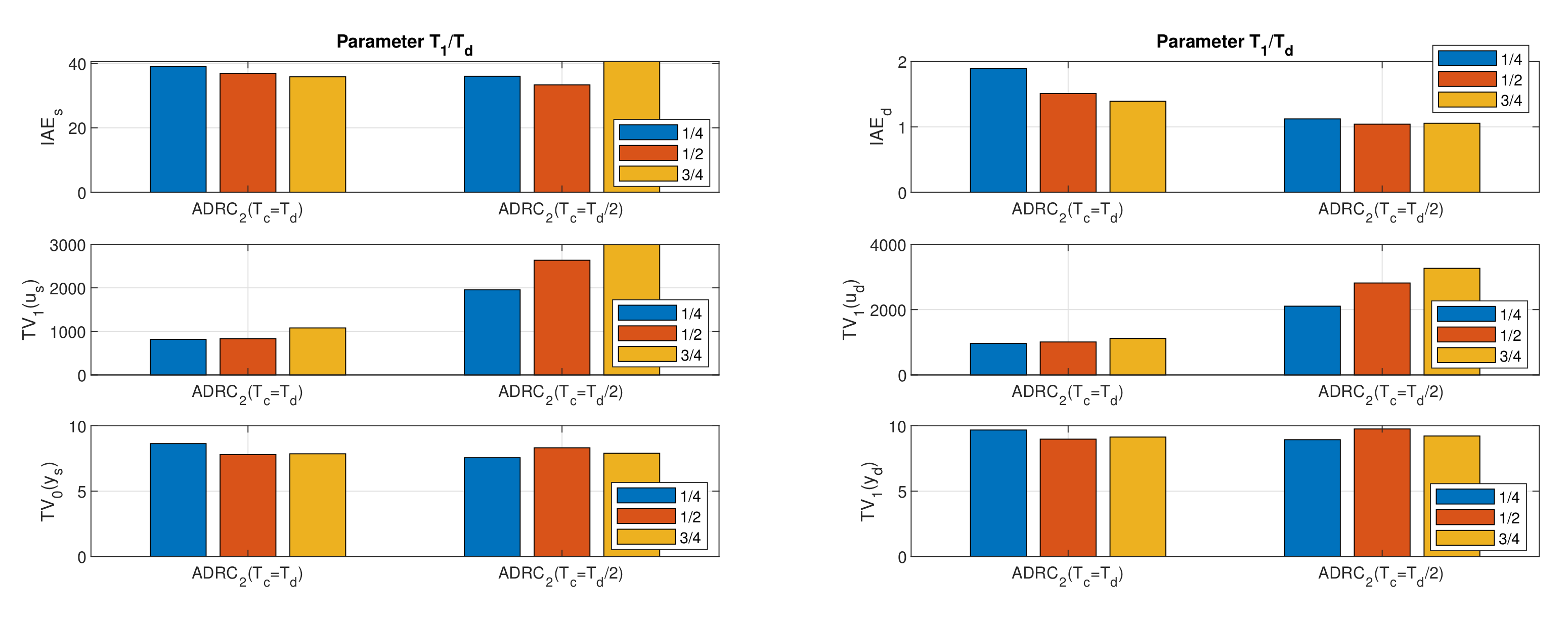
The influence of the parameter $T_1$ is different for setpoint and disturbance steps and depends to a large extent on the selected value $T_c$. For $T_c=T_d$, it affects the value of $IA{E}_s$ only slightly, while the value of $IA{E}_d$ decreases with increasing value of $T_1$. For $T_c=T_d/2$ we get the smallest values of $IA{E}_d$, which are only slightly dependent on $T_1$. However, for this $T_c$, $T_1$ has a strong impact on the excessive control effort $T{V}_1\left(u_d\right)$.

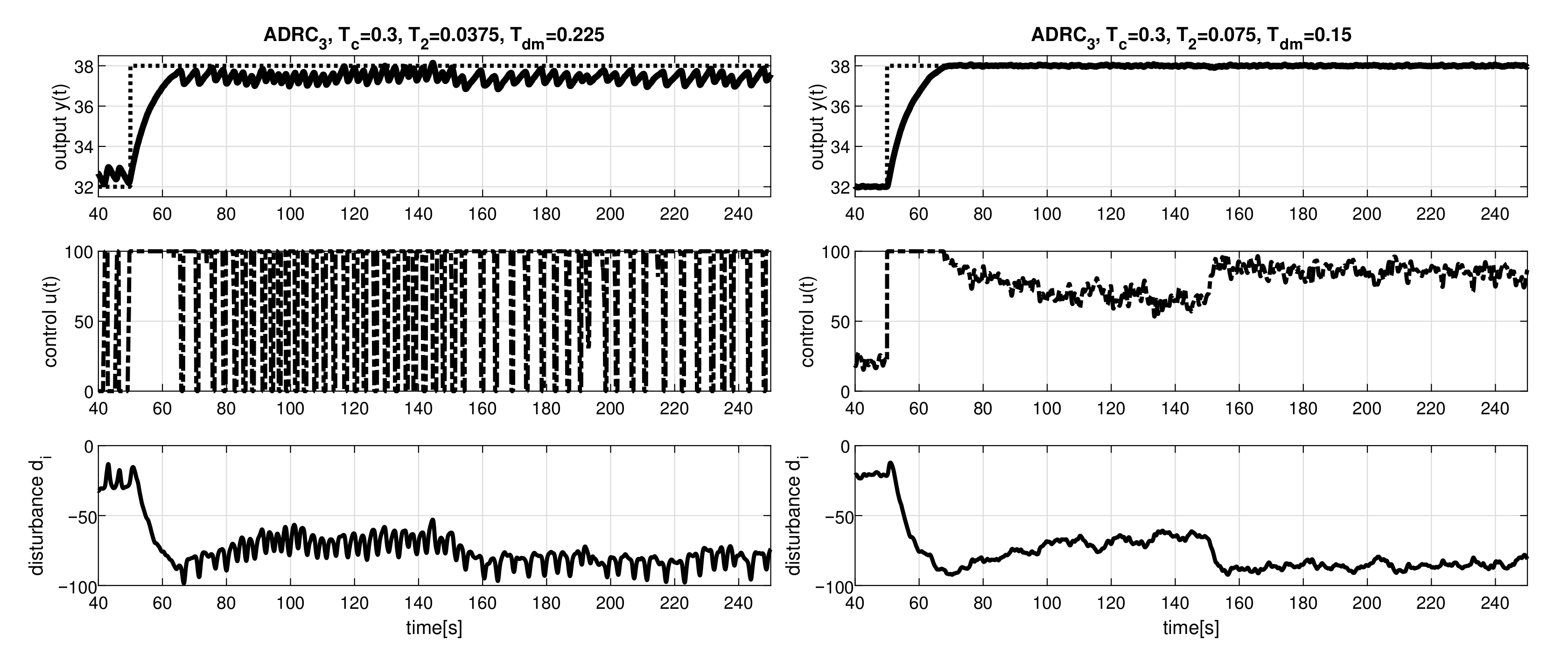
4.6. Evaluation of ADRC3

In evaluation of ADRC${}_3\left({\overline{T}}_d\right)$ controllers with the ESO delay ${\overline{T}}_d=T_d$ we will focus on choice of the ESO parameters $T_c=T_d$, $T_c=T_d/2$ and $T_c=T_d/3$. Thereby, we will analyze, how these values can be combined with the tuning parameter $T_2$. By doing so we will explore, if the ESO parameter $T_c$ should be decreased with respect to the faster dynamics of the loop with stabilizing PDA controller expressed by the time constant (23).

For the basic choice $T_c=T_d/2$, the vector of ESO time constants has been specified according to

$$T_2/T_c\in \{1/4,1/2,3/4\},\mathrm{or}{T}_2/T_d\in \{1/8,1/4,3/8\}$$

(44)

These values $T_2/T_d$ have then also been applied for the alternative tuning with $T_c=T_d$ and $T_c=T_d/3$, when the fractions $T_2/T_c$ no longer correspond to the values (44). Therefore, for simplicity, we prefer to keep the numbers $T_2/T_d$ in legends in other situations as well.

Figure 9 shows that with $T_c=T_d$ the transients can change abruptly depending on the selected value of $T_2$. With $T_2=T_d/8<<T_c$, ESO can oscillate continuously. However, increasing the value to $T_2=T_d/4$ here can already lead to high-quality transients. For $T_2=3T_d/8$ the transients would yet be smoother.

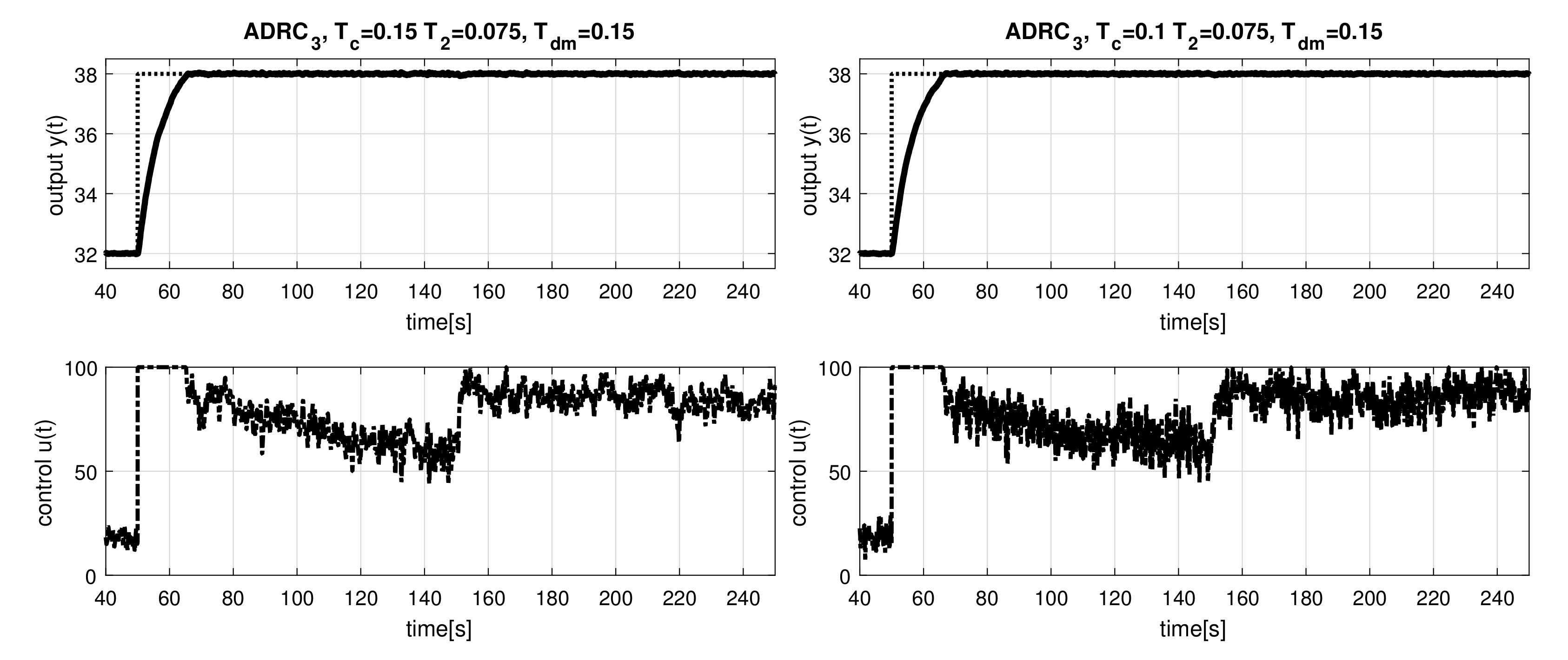
Because we are mainly interested in the question of whether it is possible to obtain faster and at the same time sufficiently smooth transients by using a higher order controller and ESO, we will focus on shorter values $T_c=T_d/2$ and $T_c=T_d/3$.

Sample of experimentally measured transients in Figure 10 and evaluation of a complete set of achieved performance measures in Figure 11 confirm intuitive expectations that, in general, decreasing $T_c$ increases the effect of noise.

However, for small values of $T_2$, shortening $T_c$ leads to a reduction in the effect of noise, and for large values of $T_2$, on the contrary, to an increase in their impact. It shows that the choice of these two parameters needs to be harmonized.

The smallest used time constant $T_2=T_d/8=0.0375$ s was only slightly larger than the sampling period $T_s=0.02$ s. At $T_c=T_d/2$, this was reflected in high excessive control effort and excessive output wobbling (Figure 11). At $T_c=T_d$, auto-oscillations even occurred in the circuit. In general, when designing controllers, it is necessary to check the condition that the used time constants are significantly larger than $T_s$ and to adapt the design of the controller or the selection of the corresponding hardware.

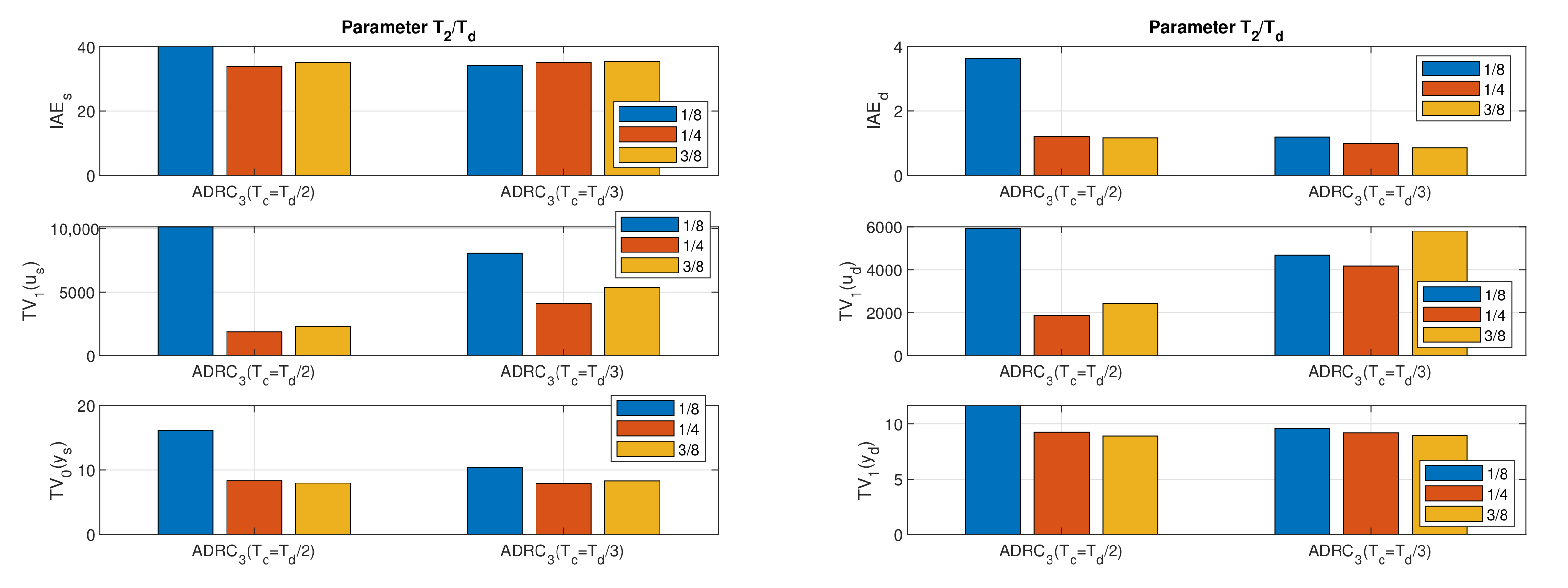
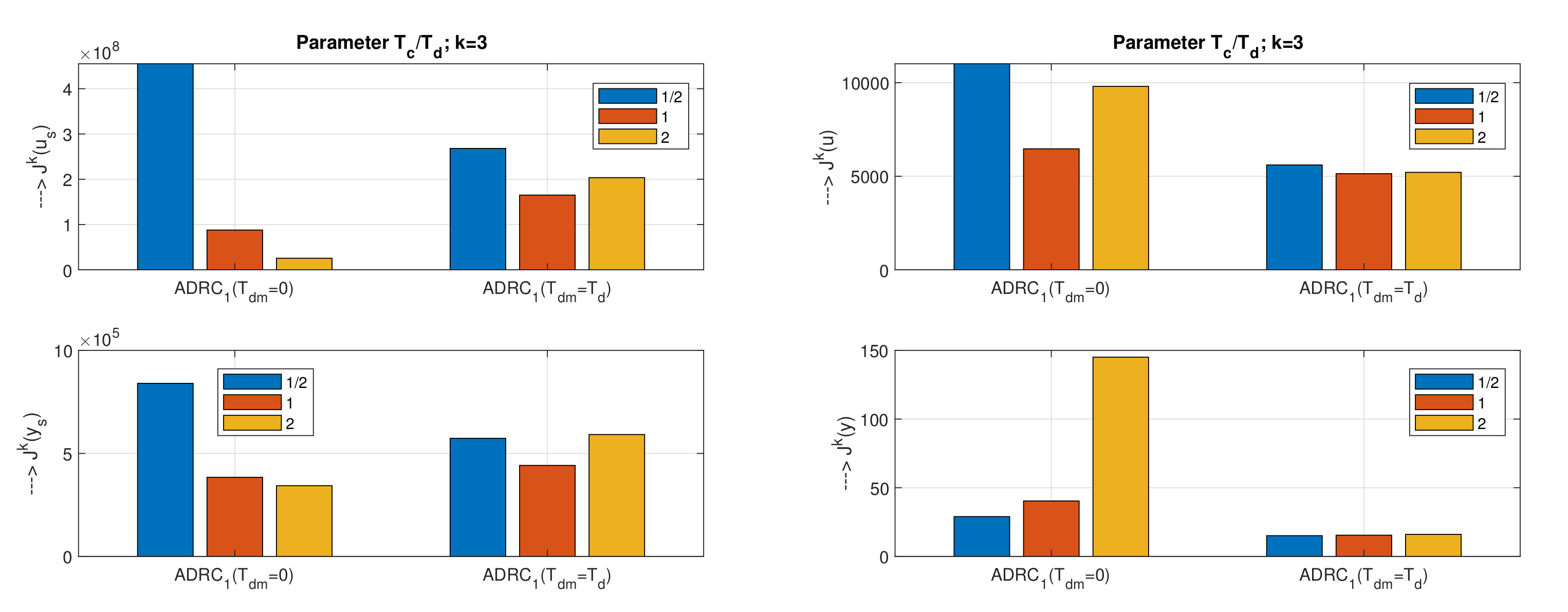
4.7. Overall Loop Optimization

In the present considerations, the individual controllers were characterized by three quantitative measures: $IAE$ (representing the speed of transients), $T{V}_1\left(u\right)$ (characterizing excessive control effort) and $T{V}_1\left(y\right)$ (excessive output wobbling), which could be related both to the setpoint and disturbance steps. When choosing the optimal solution, however, it would be far easier to use instead of these individual indicators a combined speed-effort (SE) cost function determined, for example, as

$$J_u={\alpha }_{s}IA{E}_s^{k_s}T{V}_1\left(u_s\right)+{\alpha }_{d}IA{E}_d^{k_d}T{V}_1\left(u_d\right)$$

(45)

where ${\alpha }_s$, $k_s$, ${\alpha }_d$ and $k_d$ represent appropriate weighting coefficients. Another such a combined cost function denoted as a speed-output wobbling (SW) cost function

$$J_y={\alpha }_{s}IA{E}_s^{k_s}T{V}_0\left(y_s\right)+{\alpha }_{d}IA{E}_d^{k_d}T{V}_1\left(y_d\right)$$

(46)

could focus on output evaluation. Requirements from practical applications appear to create an infinite number of different combinations of individual weighting coefficients. To illustrate their use, we will consider the simplest situations, when focussing just on the setpoint, or disturbance responses with the choice

$$J^k\left(u_s\right),J^k\left(y_s\right):{\alpha }_s=1;{\alpha }_d=0;k_s=k$$

(47)

or

$$J^k\left(u_d\right),J^k\left(y_d\right):{\alpha }_s=0;{\alpha }_d=1;k_d=k$$

(48)

Wight of the speed of the transients expressed in terms of the IAE values will be denoted by the parameter k. Next, we will compare these four parameters for two different values $k=1$ and $k=3$.

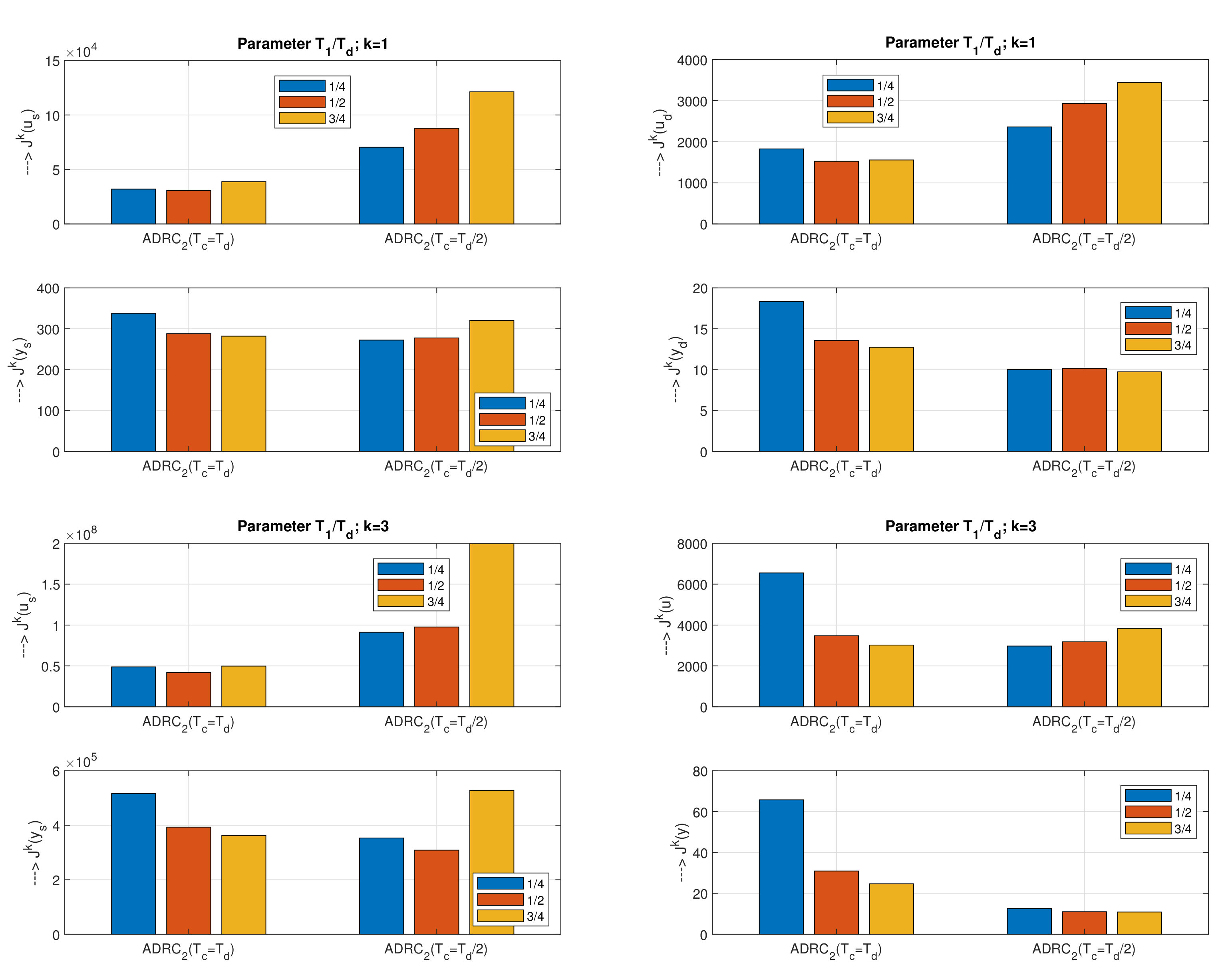
For ADRC${}_1$ controllers (Figure 12), at $k=1$ we get conclusions similar to the conclusions from the analysis of individual performance measures: higher dependence of structures with ${\overline{T}}_d=0$ on the value of $T_c$, but the possibility of reducing the cost functions by increasing $T_c$. With the tuning $T_c=2T_d$ and $k=1$ we get the globally minimal values $J^1\left(u_s\right)$ and $J^3\left(u_s\right)$.

With ${\overline{T}}_d=T_d$, the performance dependence on $T_c$ is weaker.

A low dependence of $J^k\left(u_s\right)$ values on tuning parameter $T_1$ is given by ADRC${}_2$ with $T_c=T_d$ (Figure 13). For $k=1$ and $T_c=T_d$ it holds also for $J^k\left(u_d\right)$ values. However, for $k=3$ and disturbance steps, lower $J^k\left(u_d\right)$ and $J^k\left(y_d\right)$ values correspond to the faster ESO with $T_c=T_d/2$. This controller yields the globally optimal values $J^1\left(y_s\right)$ (for $T_1=T_d/4$), $J^3\left(y_s\right)$ (for $T_1=T_d/2$) and $J^3\left(u_d\right)$ (for $T_1=T_d/4$).

Compared to ADRC${}_1$, we can state an improvement here mainly with regard to the lower dependence on the optional parameter.

Because we evaluated up to 9 settings with ADRC${}_3$ with significantly different levels of corresponding cost functions, we will omit the evaluation using bar-graphs here. The globally lowest $J^1\left(u_d\right)$ value is given by $T_c=T_d,T_2=3T_d/8$. The best $J^1\left(y_d\right)$ value corresponds to $T_c=T_d/2,T_2=3T_d/8$ and the best $J^3\left(u_d\right)$ value to $T_c=T_d/2,T_2=3T_d/8$.

Remark 3

(No globally optimal solution). We did not carry out the above analysis of the achieved solutions in order to find some specific optimal control for the given system. Rather, it was a question of whether solutions considering higher-order controllers were of any relevance to practice. The result obtained is sufficiently convincing in this respect: up to 6 of the 8 achieved best values of the possible cost functions correspond to higher-order controllers, while they are evenly distributed between $ADR{C}_2$ and $ADR{C}_3$. For them, they need to be subjected to more thorough targeted research in the future. It will probably also make sense to design and verify possible higher order controllers.

5. Discussion

In all the examples considered, the shapes of the plant input after the setpoint step change were close to the relay minimum time control and corresponded to the fastest possible energy transfer into the system. At the same time, however, the required damping of the transients could be achieved with a permissible excessive control effort and output wobbling close to the steady states.

On the one hand, the experiments show that it is easy to design fast transients even for circuits with high uncertainty, nonlinearity and non-modeled dynamics. Thereby, the example did not show all the advantages of higher order controllers, which can only manifest themselves in a relatively broad proportional zone of control (such as the differences in IAE values (26)). Due to the dominant influence of constraints, the expected benefits (such as higher robustness in the presence of uncertainty and unmodeled dynamics) do not manifest in the saturation phase covering the major part of the duration of the transients. This type of experiment was namely chosen because the evaluation with the control signal at the saturation limit is interesting to compare ADRC with other alternative solutions, such as PID with anti-windup circuit [51]. Interesting information on robustness is naturally also obtained from the dependence of the performance measures and cost functions on the tuning parameters.

Because the article focused primarily on higher order controllers, appropriate equivalents (such as e.g., presented in [22]) will need to be selected also in the prepared comparative analysis.

6. Conclusions

In the paper, several new alternatives of the simplest Active Disturbance Rejection Controllers were designed and experimentally investigated based on the approximation of the actual plant by the integrative time-delayed IPDT models. The presented new controllers expand the range of ADRC solutions suitable for time-delayed systems [12].

The main design requirement was simplicity, especially considering that the IPDT models have only two parameters and are therefore less sensitive to the selection of appropriate optional tuning parameters. Another tuning criterion was sensitivity to the measurement noise, which allows to operate with low energy dissipation near the steady states. The obtained results show that the closed loop characteristics can be significantly improved by appropriate model, controller selection and tuning.

In addition, it was shown how to implement the proposed method without complex simulations or experiments. Thereby, by a quasi-authentic illustrative example of an as fast as possible and simultaneously smooth temperature control, the dead-time compensation proposed in [33] did not prove to be the optimal solution.

The presented performance measures and cost functions, chosen to express different requirements for the transients, were used to design a set of controllers when simple IPDT models are used.

All the controllers developed may be verified by a web application and the TOM1A system used is also available for remote experimentation. It offers the possibility to verify all types of the described control algorithms. For more information, see the page http://apps.iolab.sk/advanced/appsc2020/ (accessed on 10 February 2021).