Review

Wind-Induced Phenomena in Long-Span Cable-Supported Bridges: A Comparative Review of Wind Tunnel Tests and Computational Fluid Dynamics Modelling

1
School of Civil Engineering, University College Dublin, Belfield, Dublin 4, Ireland
2
School of Mechanical and Materials Engineering, University College Dublin, Belfield, Dublin 4, Ireland
*
Author to whom correspondence should be addressed.
Appl. Sci. 2021, 11(4), 1642; https://doi.org/10.3390/app11041642
Submission received: 18 December 2020 / Revised: 2 February 2021 / Accepted: 8 February 2021 / Published: 11 February 2021
(This article belongs to the Special Issue Applications of Computational Fluid Dynamics to the Built Environment)

Abstract

:
Engineers, architects, planners and designers must carefully consider the effects of wind in their work. Due to their slender and flexible nature, long-span bridges can often experience vibrations due to the wind, and so the careful analysis of wind effects is paramount. Traditionally, wind tunnel tests have been the preferred method of conducting bridge wind analysis. In recent times, owing to improved computational power, computational fluid dynamics simulations are coming to the fore as viable means of analysing wind effects on bridges. The focus of this paper is on long-span cable-supported bridges. Wind issues in long-span cable-supported bridges can include flutter, vortex-induced vibrations and rain–wind-induced vibrations. This paper presents a state-of-the-art review of research on the use of wind tunnel tests and computational fluid dynamics modelling of these wind issues on long-span bridges.

1. Introduction

Bridge aerodynamics is a multidisciplinary field which considers the interaction between wind flows in the atmospheric boundary layer and bridges. The presence of a bridge will alter the surrounding wind environment and at the same time, the wind effects may induce bridge vibrations that can have impacts of varying levels. For long-span bridges, Fujino and Siringoringo [1] emphasise that wind is the most critical source of vibrations. This is because long-span bridges often have a long central span (for example, the Akashi Kaikyo Bridge has a central span of 1991 m), and are slender and vulnerable to the wind-induced vibrations. Furthermore, Larsen and Larose [2] note that compared with other bridge types, cable-supported bridges are even more vulnerable to wind-induced oscillations since they have more structural flexibility and less damping. An iconic example of wind-induced vibration failure is the collapse of the Tacoma Narrows Bridge which failed under a 19 m/s wind [3]. It is believed that the bridge collapsed due to the dynamic aeroelastic instability phenomenon of torsional flutter [1,4,5,6,7]. Since then, the consideration of wind effects has become an essential part in the design of modern long-span bridges, which has effectively prevented the occurrence of wind-induced bridge failures. The aerodynamic and aeroelastic features of bridges have also gained increasing research interest in the literature. Despite this, wind effects have still influenced the serviceability of long-span bridges. A recent example occurred at the Humen Pearl Bridge in China, where large oscillations of the bridge deck induced by vortices caused a complete shutdown of the bridge [8]. Therefore, the careful analysis of wind effects is paramount.
Traditionally, studies on the interactions between wind, structures, pedestrians and cyclists are carried out using wind tunnel tests. However, with improved computational power and modelling capacity, Computational Fluid Dynamics (CFD) modelling is coming to the fore as a complement to and potential replacement for wind tunnel testing. There are several disadvantages to the use of wind tunnel testing, namely the scaling issues, and the presence of physics sensors that can disrupt the flow—neither of which are concerns with CFD modelling. However, the results of CFD simulations can come with errors caused by computational codes and numerical schemes, and uncertainties brought by the assumptions made in the model. Additionally, the accuracy of CFD simulations is strongly related to the computational capacity.
The main focus of this paper is to review the state-of-the-art experimental wind tunnel and numerical CFD methods applied in the area of long-span cable bridges. Merits and existing challenges of both methods will be discussed. In addition, focus is given to the three key concerns around wind effects in long-span cable bridges which will be discussed, namely: flutter, vortex-induced vibrations (VIVs) and rain–wind-induced vibrations.

2. Background

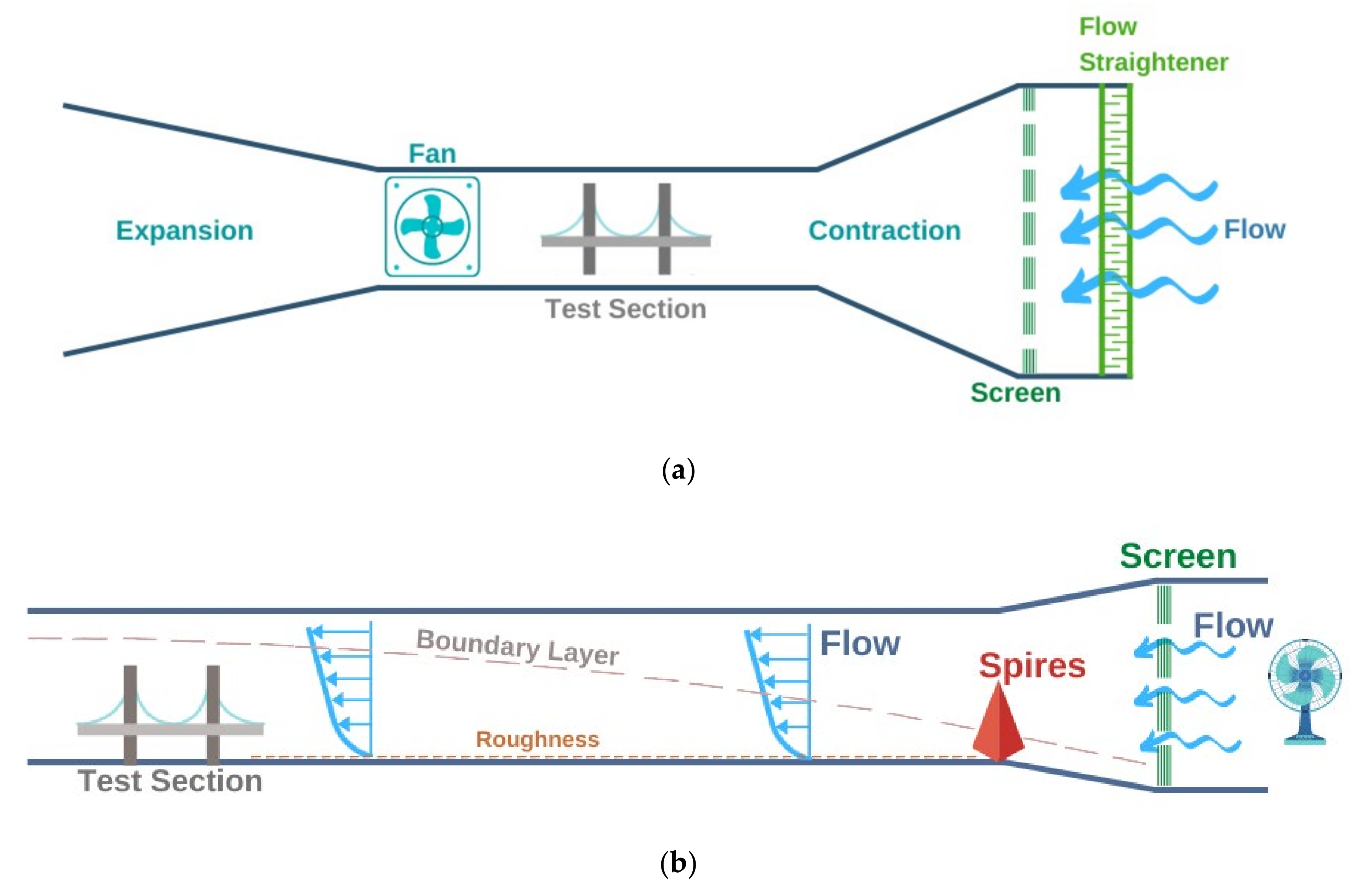
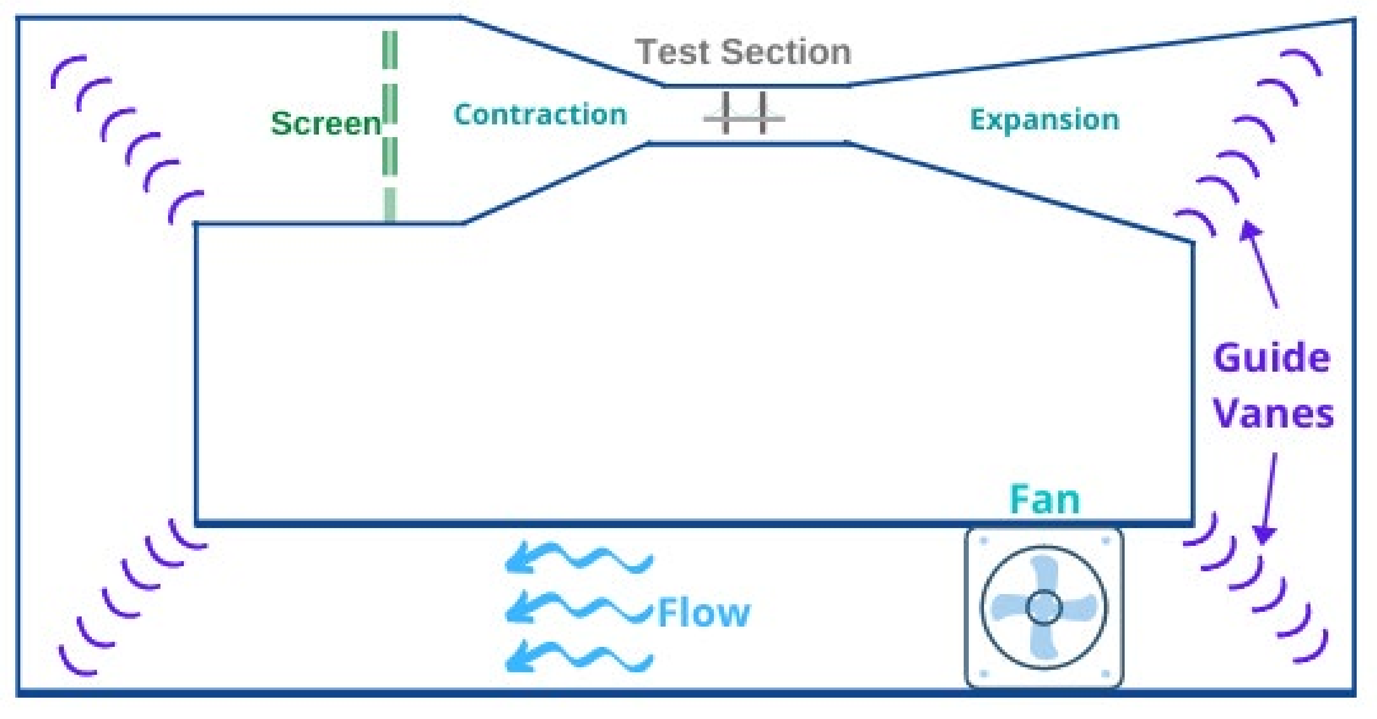
2.1. Wind Tunnel Tests

Measuring the wind effects on a structure is difficult because this process is highly sophisticated due to the random and spatiotemporally variable nature of the wind [1]. The traditional method of estimating wind effects on bridges is to conduct a wind tunnel test on a scaled model of the bridge.
The wind tunnel test was originally designed for aeronautical use and was developed during war times in the twentieth century [9]. In terms of layout, there are two types of wind tunnel: the open-circuit type and the closed-circuit type. In the open-circuit wind tunnel, air is drawn into the wind tunnel from the external environment at the inlet and discharged at the outlet, as shown in Figure 1a,b. The model to be tested can be either placed upstream of the fan (Figure 1a) or downstream of the fan (Figure 1b). The former configuration is more convenient to control the flow within the tunnel, whereas the latter is more suitable for studies where atmospheric pressure is considered important [10]. Furthermore, the latter configuration facilitates large-scale testing as the model is placed outside the tunnel. Therefore, it is often used in the study of rain–wind-induced vibrations where cables are large. Figure 2 shows the layout of a closed-circuit wind tunnel, in which the air is circulated and can be continuously accelerated within the wind tunnel. This layout is more efficient in controlling the wind velocity and requires less floor space. Hence, it is favoured in the study of bridge aerodynamics and has been normally used to derive parameters such as aerodynamic forces and flutter derivatives.
For wind tunnel tests conducted for bridges, the bridge girder, pylon or the full bridge may be validated and optimised under a given wind condition. For instance, during the design of the Stonecutters Bridge, wind tunnel tests were used to assess the impact of the complex weather conditions in Hong Kong and to subsequently refine the shape of the bridge deck [11]. Additionally, wind tunnel tests were applied to evaluate the wind effects on the bridge during its construction stage. In the construction of the Great Belt East Bridge, results of wind tunnel tests played important roles in the final decision of the erection scheme of the bridge girder [12]. During the construction of the Izmit Bay Bridge, a series of wind tunnel tests were used to assess the aerodynamic effects and confirm aeroelastic stability of the bridge [13]. More recently, before the construction of the Sutong Bridge, a series of wind tunnel tests were conducted to test the safety of the free-standing pylon and the incomplete bridge girder at the construction stage [14]. Although wind tunnel tests have been applied in the industry for many years, there are still several shortcomings and limitations of using this method to study bridge aerodynamics. Firstly, bridges are large structures. To test them in a wind tunnel, small-scale models are needed to be able to fit in a wind tunnel facility. The common range of scales used in wind tunnel tests for bridge models is 1/50 to 1/200 [9]. However, Larsen et al. [15] indicated that such small scales cannot provide reliable results for the study to mitigate VIV. Resulting from the small scale, the fluid boundary layer at structures such as guide vanes and deflectors on the bridge model will become too thick relative to the size of these structures, which will significantly influence the flow rate near these structures. For cases that require high resolutions of boundary layers, large-scaled sectional models should be used. However, the dimensions of the testing model in a wind tunnel are limited by the size of the testing facility and a factor termed the “blockage ratio” (the ratio of the cross-sectional area of the test model to the cross-sectional area of the wind tunnel). According to Holmes [9], a recommended blockage ratio of less than 5% should be achieved to acquire faithful results. Hence, it is difficult to obtain a full-scaled Reynolds number in wind tunnels. Secondly, the existence of sensors and other structures such as end plates might interfere with the flow field, and measurements can only be taken at sensor locations which must be chosen in advance. Kubo et al. [16] have proved that the size of endplates used in two-dimensional (2D) wind tunnel tests has a large impact on the results. In their experiment, when the blockage ratio was close to 0.15, a combined effect of the endplate and the high blockage ratio led to an overestimation of the drag force on the model. Reddy et al. [17] also showed that endplates might have a significant effect on flow separations. Another limitation is the approximation of the natural wind characteristics in the wind tunnel, especially the approximation of the inlet condition. To gain a similar velocity profile and turbulence intensity of the natural wind at the inlet, the wind tunnel should provide enough roughness at the wall. This can be achieved by installing fixed grids and spires at the inlet and other roughness elements along the testing section so that the turbulence can be generated passively. Due to the simplicity of the setup, the passive method is used in most bridge wind tunnel tests. However, this method is only suitable for long testing sections. Simiu and Scanlan [18] suggest that the implementation of passive turbulence generation in short wind tunnels will lead to questionable results as the turbulence is not fully developed. There have been attempts to incorporate active controlling systems into the generation of inlet turbulence. For instance, Hideharu [19] designed the first active grid turbulence generator which allows accurate control of the inlet flow by dynamically adjusting the opening of the grid. It is commonly accepted that the active controlling strategy yields better results than the passive method. However, due to the cost, there has not been any research highlighting the implementation of active turbulence control in bridge wind tunnel tests. Finally, the cost of wind tunnel tests can be high. In addition to the expensive maintenance cost of the wind tunnel facility, wind tunnel tests are often repeatedly conducted during bridge design. Additionally, a small change in the bridge structure could lead to a series of costly wind tunnel tests for validation.

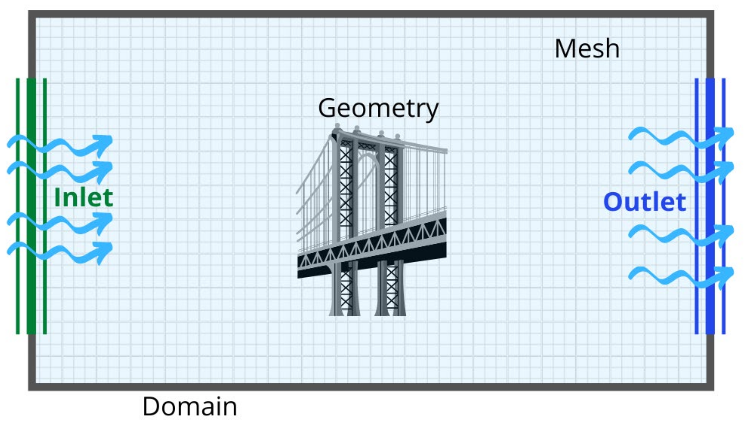
2.2. CFD Simulations

Computational Fluid Dynamics (CFD) is a branch of fluid mechanics that utilises the computational power of modern computers to model fluid flow (Figure 3).
The essence of the method is to numerically solve partial differential equations that govern the conservation of mass, momentum and energy of fluids. In the study of bridge aerodynamics, the air is often assumed to be incompressible, Newtonian and isothermal. Therefore, the air is governed by the momentum equation, Equation (1), and the continuity equation, Equation (2),
u t + u u = p + ν 2 u + g
u = 0
in which, u is the velocity vector, p is the kinematic pressure, ν is the kinematic viscosity and g is the gravity as a source term. Equations (1) and (2) are known as the Navier–Stokes equations. By solving these two equations, the fluid velocity and fluid pressure at points of interest in a flow can be determined. Simulations based on Equations (1) and (2) directly are called direct numerical simulations (DNSs). Although DNSs are very accurate in solving simple flow problems, they are inefficient for practical problems due to the significant requirement for computational power. In practice, the Reynolds-Averaged Navier–Stokes (RANS) formulation is often used as a replacement of the original Navier–Stokes equations,
u ¯ t + u ¯ u ¯ = p ¯ + v 2 u ¯ + g + u u ¯
u ¯ = 0
where u ¯ is the time-averaged velocity, p ¯ is the mean kinematic pressure and u is the fluctuation velocity. Compared to Equation (1), Equation (3) has an extra term u u ¯ , in which u u ¯ is known as the Reynolds stress. To close the equations, the Reynolds stress must be approximated using so-called turbulence models.
The most commonly used turbulence models in bridge aerodynamics are eddy-viscosity models, in which the Boussinesq hypothesis is applied so that the Reynolds stress can be calculated by the mean velocity field and the turbulence viscosity. These models normally contain one or two transport equations, and so the computational cost is relatively low. Table 1 lists a few frequently used eddy-viscosity models.
Among the models listed in Table 1, the k-ε models are particularly favoured in applications related to civil and structural engineering. In order to validate the use of k-ε models in the built environment, Murakami and Mochida [30] conducted a pioneering study to examine the accuracy of results derived from RANS simulations with the standard k-ε model. Three-dimensional steady-state simulations with various mesh schemes and boundary conditions were performed on a cubic geometry. By comparing results from these numerical simulations to wind tunnel results, it is found that RANS simulations using the standard k-ε model can faithfully reproduce the velocity field and pressure field measured in wind tunnel tests if configured with sufficiently fine mesh and compatible boundary conditions. This study emphasised the significant effect of the mesh and boundary conditions on numerical results, and also showed the enormous potential of CFD simulations. However, a study by Tominaga et al. [31] showed that the standard k-ε model and its variants can overestimate the reattachment length behind the bluff body compared to experimental results, which is considered a common drawback of using the k-ε model. Spalart–Allmaras models are another group of models favoured in engineering applications because only one transport equation is introduced. However, the limitation of this model is significant. Pope [32] indicates the model is designed for specific airfoil simulations and not suitable as a generalised turbulence model. This is also shown by Richards and Norris [33] who suggest that the Spalart–Allmaras model overpredicts the wind pressure in a channel-flow simulation. In engineering practice, it is essential to calibrate the Spalart–Allmaras models before their implementation, which is normally based on experimental data. More recently, there have been some attempts to use machine learning techniques to calibrate parameters used in the model [34,35]. Despite the large progress made in eddy-viscosity turbulence models, there are still some limitations. Pope [32] suggests that for cases with large streamline curvature, strong fluctuations or large flow circulations, eddy-viscosity models might deliver unphysical results in the vorticity. Instead, Reynolds stress turbulence models, which directly resolve transport equations of Reynolds stress without the Boussinesq hypothesis, will perform better with strong turbulent flow. Many models have been developed based on two fundamental models, the LRR model by Launder et al. [36] and the SSG model by Speziale et al. [37]. Interested readers are referred to a review paper by Argyropoulos and Markatos [38]. However, Reynolds stress models normally contain more transport equations than eddy-viscosity models. For instance, a recent blended model of LRR and SSG by Klajbár et al. [39] contains six transport equations and one additional equation to close the solution, which makes the computation significantly slower than using two-equation eddy-viscosity models. Therefore, it is necessary to balance between the efficiency and the accuracy in the selection of turbulence closure for the RANS formulation.
RANS simulations with appropriate turbulence models can provide sufficiently accurate results in the study of time-averaged wind effects. However, for cases with large flow separations and vortex shedding, transient simulations that reflect the unsteady nature of turbulence should be adopted. Although the RANS formulation can be used to perform transient simulations, i.e., the unsteady RANS (URANS) simulations, Baker et al. [40] suggest that URANS might smooth the fluctuation caused by vortices as the velocity field is time-averaged. A more accurate approach is the large-eddy simulation (LES), which was originally developed by Smagorinsky [41] to study unsteady atmospheric motions. This meteorological approach was later examined and extended for general engineering implementations by [42]. Unlike the RANS formulation that uses Reynolds averaging to reduce the computational cost of DNSs, a LES applies a low-pass filter to the flow field so that motions of large-scale eddies can be fully resolved, and vortices of small length scales are modelled. It is arguably the most accurate transient approach next to the DNS, while still being applicable to real life problems. Murakami and Mochida [43] showed that URANS, in general, cannot produce faithful results of vortex shedding in the wake region of a bluff body compared to experimental results, while 3D LESs can accurately reflect the fluctuations in velocity and pressure field of the unsteady flow. It was also shown through a comparison of 2D and 3D LESs that 2D LESs of a bluff body geometry would yield inaccurate results of fluctuating pressure and velocities, leading to large discrepancies in aerodynamic forces compared to experimental results and 3D LES results. Despite its affordability compared with DNSs, a LES is still computationally demanding as it inherits the strong grid number-dependent feature of DNSs. An appropriately configured LES normally requires finer mesh than an equivalent URANS simulation. In a comparison between URANS and LES by Som et al. [44], LES takes ten times the CPU hours of a URANS simulation with only doubled grid points. To reduce the computational cost of transient simulations, Spalart et al. [45] proposed the detached-eddy simulation (DES) approach which applies URANS to model the boundary layer and LES to resolve the turbulence in the trailing end. Based on the original formulation, there have been improved versions: the delayed-detached-eddy simulation (DDES) by Spalart et al. [46], the improved DDES (IDDES) by Shur et al. [47] and the modified IDDES by Han et al. [48]. It can be summarised that the LES- and DES-based methods will be the best options for transient simulations before DNS becomes affordable.
In the study of bridge engineering, CFD models are used in the study of aerostatic, aerodynamic and aeroelastic performances of bridges. Compared to wind tunnel tests, the CFD method has several advantages in this area. Firstly, there is no physical limit in the size of the testing domain and geometries, which makes full-scale simulations possible. Therefore, the consistency of the Reynolds number can be maintained. Secondly, CFD simulations provide nonintrusive data collection from every point within the testing domain. This is essential to the study of aeroelastic problems, in which a large amount of data are generated simultaneously in both the solid region and the fluid region. Finally, CFD simulations are highly flexible in terms of the cost. Based on the objectives and the budget of a task, CFD can offer wide ranges of solutions from RANS simulations that are significantly cheaper than wind tunnel tests to LESs that are computationally expensive. Despite the advantages of the CFD simulation, its implementation in bridge aerodynamics is still not as popular as the wind tunnel test because of a few limitations. Firstly, unlike the wind tunnel test that has been incorporated in bridge design for decades, the CFD method is a relatively younger technique introduced in this area. Although the application of CFD in the aeronautics provides a lot of experience for bridge CFD practice, there is no standard or guide to follow for bridge CFD simulations. Therefore, validation is still required to provide confidence in the predictions, particularly related to the choice of turbulence model and numerical settings. Secondly, although steady-state simulations are normally much cheaper than a wind tunnel test, the computational cost of high-resolution transient simulations is still high. For instance, a transient simulation with billions of cells on 64 CPU cores can take a few weeks to finish, which might cost over USD 400 per week [49]. In addition to the computational cost, CFD simulations also generate massive amounts of data, which makes postprocessing challenging. In the following sections, the application of both wind tunnel tests and CFD simulations in the study of bridge aerodynamic and aeroelastic problems are reviewed.

3. Aeroelasticity and Aerodynamics of Cable-Supported Bridges

Long-span cable-supported bridges are normally slender and flexible structures of large mass and are more vulnerable to dynamic issues given the resulting low levels of structural damping and natural frequencies. Fujino and Siringoringo [1] highlight that wind is the most critical source of vibrations on long-span bridges. The most commonly observed aeroelastic and aerodynamic phenomena in long-span bridges are flutter and vortex-induced vibrations (VIVs) in the deck, and rain–wind-induced vibrations (RWIVs) in the cable system.

3.1. Flutter—Aeroelasticity of the Deck

3.1.1. Mechanism of Flutter

Scanlan and Tomko [50] used the term flutter to describe the wake oscillation that occurs on bridge decks and compared this to similar vibration patterns found on propellers and airfoils. It is an instability that starts to grow when the structural damping cannot resist dynamic effects of aeroelastic forces induced by the relative angle of attack [9]. Xu [10] extends this explanation from an energy perspective:
“If the energy input by the aerodynamic forces due to strong winds in a cycle is larger than that dissipated by the damping in the bridge structure system, the amplitude of vibration of the bridge deck will increase. This increasing vibration will then amplify the aerodynamic forces, resulting in self-excited forces and self-exciting oscillations. The vibration amplitude of the bridge deck can build up until it results in the collapse of the bridge.”
Different from the VIVs that only occur at certain frequencies, flutter will grow in time after the ambient flow has passed the critical velocity [51], which will lead to divergent oscillations that can be catastrophic. In the case of the Tacoma Narrows Bridge (Figure 4), severe vibrations were observed before the collapse. Since then, flutter instability has drawn significant attention.
Scanlan [4] developed the fundamental flutter theory, in which flutter is described as a self-excited aeroelastic instability with divergent vibration amplitude. The divergent characteristic of vibration is due to the coupling between structural motions and unsteady aerodynamic forces—namely, the lift force, drag forces and the pitching moment [1]. To quantitatively describe the relationship between the aeroelastic forces and the unsteady motions, Scanlan [4] introduces flutter derivatives which are functions of the dimensionless velocity and frequency. In bridge design, flutter derivatives are employed to determine the critical flutter velocity of a bridge deck and thus determine if a bridge is susceptible to flutter. Therefore, it is essential to accurately identify these parameters. The bridge deck is a three-degree-of-freedom (3-DOF) system that has lateral, vertical and torsional displacements. Since it was challenging to design a 3-DOF suspension system for the experiment, early research normally simplified the bridge deck into a two-degree-of-freedom (2-DOF) system that would ignore the lateral displacement. However, ignoring the lateral displacement is not suitable for long-span bridges as they normally have relatively low lateral stiffness. Decades of development in the apparatus has enabled the state-of-the-art research to study all 18 flutter derivatives of a 3-DOF system in three-dimensional (3D) coordination.

3.1.2. Wind Tunnel Studies of Flutter

Conventional approaches in assessing flutter are based on experimental wind tunnel tests which can be classified into two categories: the free vibration method and the forced vibration method.
(1)
Free vibration wind tunnel tests
The free vibration method was first proposed by Scanlan and Tomko [50] to identify eight flutter derivatives of a 2-DOF bridge deck system. In this method, a sectional model is spring mounted in a wind tunnel where modal tests under various wind conditions are performed. Flutter derivatives can be identified from the recorded motions and corresponding wind conditions. Detailed mathematical derivation can be seen in the work of Scanlan [4]. Given that flutter can occur in heave, pitch and sway directions of the bridge deck, Chowdhury and Sarkar [53] extended Scanlan’s theory to present a framework for the 3-DOF free vibration method. The free vibration method requires only a simple apparatus, and therefore is a low-cost option (given there is no need to record the aerodynamic forces acting on the testing model).
There are, however, challenges associated with free vibration tests in wind tunnels reported in the literature, particularly in the estimation of flutter derivatives at high wind velocities [54]. As the wind velocity increases, the aerodynamic damping effect in the vertical mode becomes so high that vibrations of the model are too small to be accurately recorded. Although they proposed using models with larger mass values to solve this, the increased mass value is strictly limited by the capacity of the suspension system used in the test. Ding et al. [55] aimed to identify flutter derivatives from complex modal parameters; however, they only showed that this method could analyse cases of high velocity on idealised thin-plate sections. Despite recent improvements in sensor technology, this problem still exists in state-of-the-art free vibration tests [56]. Scanlan [57] showed that flutter derivatives can be affected by the turbulence intensity and since the turbulence condition also depends on the wind velocity, most free vibration tests are performed under smooth air.
(2)
Forced vibration wind tunnel tests
Compared to the free vibration method, the forced vibration method requires less mathematical effort but more experimental data. In the free vibration method, only the displacement of the testing model is recorded, while during the forced vibration method, both the displacement and forces acting on the model are recorded simultaneously, and ultimately the flutter derivatives can be directly identified. The main advantages of using the forced vibration method are its simplicity in extracting flutter derivatives, its adherence to the theoretical framework and its greater control of the oscillation amplitude. Therefore, the forced vibration method has become a popular option in the industry. For instance, during the design of the Musi III cable-stayed bridge, a series of wind tunnel vibration tests were performed to determine the flutter derivatives and critical flutter velocities of the bridge [58]. However, the wind tunnel forced vibration test has some significant limitations. Firstly, it is essential to simultaneously record the unsteady signals of dynamic forces and structural motions during the test. To achieve this, a complex apparatus is required, such as high-frequency balance, electronic scanning valve and sensors to record acceleration and displacement. This can potentially increase the instrumental error. Secondly, the accurate extraction of aeroelastic forces from recorded dynamic forces is challenging. The total forces recorded in the experiment can include not only inertia forces and mechanical interference forces, but also buffeting forces caused by turbulence. Siedziako, Øiseth and Rønnquist [59] conducted and experiment in smooth air conditions to neglect the buffeting forces. Niu et al. [60] limits the turbulence intensity to 0.01 in their forced vibration test. However, such a solution will limit the test to a relatively low wind velocity condition where turbulence effects can be neglected. This also leads to the third limitation of the forced vibration method. Xu and Zhang [61] suggest that to perform a forced vibration test at high wind velocity, the sectional model should be highly rigid and light in weight. However, these two factors are normally incompatible in an experimental condition.

3.1.3. CFD Studies of Flutter

Wind tunnel studies have constituted the bedrock for research of flutter instability. Great achievements have been made in revealing the underlying mechanism and providing valid frameworks to predict the onset of flutter. However, limitations caused by apparatus have been witnessed, especially in the identification of flutter derivatives at high wind velocities. Therefore, numerical simulations that inherit the frameworks of the wind tunnel tests have gained research interest in this area.
(1)
Forced vibration simulations
The first attempt to combine experimental wind tunnel methods and modern numerical simulations in the study of flutter on bridge deck was made by Brar, Raul and Scanlan [62]. They extracted eight flutter derivatives of a 2-DOF airfoil section by conducting URANS simulations using the standard k-ε turbulence model and the finite element method. The bridge surface was treated as a no-slip wall where the near-wall treatment was fulfilled by applying a wall function on the thick near-wall elements that contained the viscous and transitional sublayers. Compared with currently available computational capacity, these simulations would be considered nascent for using a 2D coarse mesh and approximating the near-wall behaviour using wall functions. This turbulence model has been demonstrated to poorly represent the near-wall regions and the numerical scheme only offers first order of accuracy. Nonetheless, the results are shown to agree well with analytical results even in the high-Reynolds number condition where the flow becomes turbulent. Additionally, applying the no-slip wall condition at the bridge surface has become a common practice in the study of bridge aerodynamics. Szabo, Gyorgyi and Kristof [63] identified eight flutter derivatives from a 2-DOF system using 2D URANS simulations. The standard k-ε turbulence model was used, although the configuration of the near-wall region was not specified. A dynamic mesh was used so that the sectional model could move in vertical and torsional directions. Compared to results of a forced vibration wind tunnel test and analytical results, their simulations give similar results when estimating the self-excited forces, structural motions and the flutter derivatives. Furthermore, a 3D fluid-structure-interaction (FSI) simulation was performed to determine the critical flutter velocity. While the results have shown agreement with those from the wind tunnel test, there are some limitations to the work. The geometry was an idealised thin-plate section without handrails and barriers. A “much coarser mesh” was used than that in the 2D simulation, which could potentially compromise the accuracy of the results. Additionally, the wind field was conducted using a URANS simulation with the k-ε turbulence model, which represents a compromise of accuracy in favour of simulation efficiency. Sun, Owen and Wright [64] suggest that the use of the k-ε turbulence model could create excessive turbulent kinematic energy as wind makes contact with the bridge deck, which could substantially compromise the flow. It was also suggested that the k-ω model and its variants are better for URANS simulations of flutter because the energy dissipation frequency ω can maintain a nonzero value in the near-wall region which allows for direct integration in the viscous sublayer. A 2D URANS simulation was conducted on a rectangular cylinder with the standard k-ω turbulence model. Instead of using wall functions at the boundary layer, they adopted a fine mesh that resolves the viscous sublayer. The 18 flutter derivatives of the 3-DOF system were derived from the simulations using the forced vibration method and good agreement was found compared to the wind tunnel results. Šarkić, Höffer and Brčić [65] emphasise that the application of an appropriate turbulence model is essential to the accurate estimation of aeroelastic forces. Three-dimensional LESs were conducted using the dynamic Smagorinsky subgrid model and 2D URANS simulations were conducted based on the k-ω SST turbulence model to study how different turbulence modelling techniques can affect the results of flutter derivatives derived from numerical simulations. In general, results of both the 2D URANS simulations and the 3D LESs were in good agreement with the experimental data, although the LESs provided a closer match to the experimental results. However, compared to the experimental data, discrepancies were found in two damping-related flutter derivatives derived from both the LESs and the URANS simulations. By studying the distribution of pressure amplitudes and pressure phase angles, large differences between URANS results and experimental results were found to be caused by the limitation of the URANS method in the representation of flow separation. This finding suggests that the use of 2D URANS simulations with the k-ω SST turbulence model might not be suitable to accurately identify flutter derivatives. However, the comparison was not extended to include the application of other eddy-viscosity models and Reynolds stress models in the URANS method, which might provide some insights into the topic. It was also found that the discrepancies between the LES results and the experimental results were caused by the larger separation bubbles in the simulations, which is suggested to be a result of the smooth incident flow condition used in the LESs. Furthermore, it was shown that the LESs consumed more than 10 times the CPU hours of the 2D URANS simulations. In addition, 3D URANS simulations were not conducted which might be more computationally affordable than LESs and provides better results than 2D URANS simulations. Mannini, Sbragi and Schewe [66] performed a series of 2D URANS simulations to study the dependence of flutter derivatives on various factors. A comparison was made between an eddy-viscosity model, the one-equation Spalart–Allmaras model, and a Reynolds stress model, the linearised explicit algebraic (LEA) model. It was found that the Reynolds stress model delivered slightly better results than the Spalart–Allmaras model. By comparing these results to the experimental results from a free vibration test, large discrepancies were found at high velocities in the values of the two flutter derivatives related to aerodynamic damping. These discrepancies were caused by the difference in the mean angles of attack used in the simulations and in the wind tunnel tests. After replacing the mean angle of attack in the simulations by the value used in wind tunnel tests, the discrepancies were almost eliminated. The study was further extended to compare two different configurations of the bridge deck section—a smooth edge with a rounded shape and a sharp edge that had a higher bluffness. By incorporating both geometries into the simulations, it was found that the smooth-edge geometry with a large mean angle of attack had similar flutter derivatives to the section of the sharp-edge geometry. The author also emphasised the important role of the Reynolds number on flutter derivatives and found that bridge decks might have a dramatic change in flutter derivatives within Reynolds number range of 1 × 10⁶ to 5 × 10⁶. When increasing the Reynolds number up to 1 × 10⁸, the effect of negative aerodynamic damping tended to decrease. Therefore, it was necessary to include high-Reynolds number wind tunnel tests in the experimental measurement of flutter derivatives. Similarly, Helgedagsrud et al. [67] identified flutter derivatives through a series of 3D forced vibration simulations based on the Arbitrary Lagrangian–Eulerian Variational Multiscale (ALE-VMS) formulation of the Navier–Stokes equations for incompressible flows, which offers a convenient FSI framework based on the finite element approach. In the ALE-VMS method, the turbulence is computed similarly to that in LES, where large-scale eddies are fully resolved, and subgrid eddies are modelled. Hence, the turbulence behaviour can be reflected with satisfactory accuracy. However, their computational domain is a slice of the wind tunnel they are comparing and only contains a limited number of cells in the transverse direction. While this saves on computational power, it is arguable whether it is accurate enough in terms of the spatial discretisation since they did not provide any sensitivity study to justify their choice of the computational domain and mesh. Combined with nonpenetration boundary conditions configured at walls, their computational domain might limit the development of the flow in the transverse direction, which could possibly influence the accuracy of the results of the 3D simulations. Tang, Shum and Li [68] performed a flutter analysis using forced vibration numerical simulations on twin-box girders. Two-dimensional URANS simulations were conducted with the k-ω SST turbulence model. Flutter derivatives were determined for girders with three different slot widths under different mean angles of attack. It was found that under zero mean angle of attack, the larger central slot width can effectively increase the critical flutter velocity. However, when considering the larger mean angle of attack, the presence of the central slot will significantly reduce the critical flutter velocity for torsional flutter. Increasing the slot width will further reduce the critical flutter velocity, making the deck more prone to torsional flutter. However, the simulations are only 2D and use URANS with an eddy-viscosity model and validation was only performed for a stationary bridge deck with steady-state wind tunnel tests in terms of mean streamwise velocity field. Comparisons between numerical results with flutter derivatives derived from aeroelastic wind tunnel tests were not presented which makes the findings potentially unreliable.
(2)
Free vibration simulations
Xu and Zhang [61] appear to be the first to incorporate the free vibration method into CFD simulations. They performed 2D URANS simulations with the k-ω SST turbulence model on three different geometries—an idealised thin-plate deck, a trapezoidal deck and a streamlined deck with lateral cantilevers. The simulation results of the thin-plate deck agree well with the analytical solution. However, when comparing the results of the other two geometries with the corresponding forced vibration tests, moderate discrepancies were found at high velocities. For the trapezoidal deck, the discrepancies were found in the flutter derivatives related to the heaving motions. It was suggested that this could be due to the larger mean angle of attack in the free vibration simulation due to high torsional moment coefficients at high wind velocities, which supports the findings of Mannini et al. [66]. For the streamlined deck, the discrepancies were mainly found in the flutter derivatives that are related to the coupling effect between torsional vibrations and vertical vibrations. It was suggested that this was due to the nonlinear nature of the aeroelastic forces which cannot be fully reflected in the commonly used linearised flutter theory. Wu, Kareem and Ge [69] present frameworks for bridge aeroelasticity with a strong focus on nonlinearity. Their simulations were based on a 2D mesh although it is widely accepted that by its nature, turbulence tends to develop in three dimensions. Using a 3D turbulence model in 2D simulations will significantly influence the accuracy of the results [70].

3.1.4. Summary

Early-stage free vibration wind tunnel tests revealed the fundamental mechanism of flutter and helped establish flutter theory. However, forced vibration wind tunnel tests have been more popular in the study of flutter. As a result of limitations in experimental setup, both free vibration and forced vibration wind tunnel tests have not yet been able to deliver faithful results of flutter derivatives at high wind velocities.
Research on the application of CFD simulations in flutter analyses is wind-ranging. Most studies adopt the forced vibration framework in simulations which is commonly accepted as a robust method, especially at higher wind velocities. Furthermore, imposed bridge deck motions in a forced vibration framework are easier to control than those in a free vibration method, leading to a saving in computational effort. There are several limitations in the state-of-the-art literature on this topic. Firstly, most studies adopt the URANS method, which averages the fluctuations in the flow field. Secondly, most studies that use the URANS method apply eddy-viscosity turbulence models, which might be used to deliver sufficiently accurate results of global forces and velocity distribution but might oversimplify the flow circulations. It is apparent that the aforementioned limitations are compromises made to save computational power. Extensively performing 3D LESs with high-fidelity geometries is still challenging. However, there are some methods that are more affordable yet provide better results than URANS with eddy-viscosity models, such as DESs, and URANS simulations with Reynolds stress turbulence models. Flutter is sensitive to the geometry and turbulence model, and hence a comprehensive sensitivity study considering various turbulence model techniques and more realistic geometries will largely improve the application of CFD simulations on this topic.

3.2. Vortex-Induced Vibration

3.2.1. Mechanism of Vortex-Induced Vibration

Vortex-induced vibrations (VIVs) are motions induced on a structure which is interacting with an external flow and are produced by vortex shedding of the flow [71]. When the wind velocity is beyond a critical value and within a critical range, the interaction of flow and bridge deck will produce a “lock-in” effect that synchronises the vortex shedding frequency with the frequency of the structure [51]. Holmes [9] summaries the four conditions under which VIVs can occur:
(1)
The wind has a normal direction to the longitudinal axis of the bridge deck.
(2)
The turbulence intensity is normally less than 5%.
(3)
The critical wind velocity is within the range of 5 to 12 m/s.
(4)
The damping ratio of the system is less than 1%.
It should be noted that VIVs only occur at a critical range of wind velocity, which indicates the vibration will not develop divergently, and so has not yet destroyed any bridges. However, it is commonly accepted that VIVs tend to accelerate fatigue damage and failure under serviceability criteria. It is reported that vibrations of large amplitudes are a common occurrence. For instance, a VIV was observed on the section model of the Stonecutters Bridge during the design stage [15]. The Great Belt Bridge encountered a series of VIVs during the construction of the girder, of which the maximum amplitude reached 0.32 m at the main span that is 1624 m long [72]. Similarly, VIVs with amplitudes of over 0.5 m occurred on 240 m spans of the Trans-Tokyo Bay Bridge after the girder was fully constructed [73].

3.2.2. Wind Tunnel Studies of Vortex-Induced Vibrations

There has been a significant amount of research into the use of wind tunnel tests for investigating VIVs. Experimental studies have been categorised into two groups depending on their focus: investigations on how to faithfully reproduce VIVs in wind tunnels and studies to find effective suppression strategies of VIVs.
(1)
Reproducing VIV in wind tunnel tests
Matsumoto [74] classified vortex shedding effects of bridges into three mechanisms: one-shear-layer vortices, which are normally seen on the bridge deck and girder, two-shear-layer vortices, and 3D vortices, which are commonly observed in cable vibrations. They emphasise the vital role of the boundary layer in the formation of VIVs. It is suggested that the mechanism of creation or suppression of VIVs can be explained by the “double vortex mode” [75]. The “double vortex mode” considers effects of two types of vortices, those formed by model motions and those formed by secondary motions. The separation of these vortices generates periodic aerodynamic forces on upper and lower surfaces of the bridge girder which will constantly move the girder in the vertical direction. Helgedagsrud et al. [76] suggested that the study of VIVs and flutter instability are interdependent. For instance, twin-box girders are a new type of bridge girder designed to suppress flutter by increasing the critical flutter speed. However, Larsen et al. [15] proved that twin-box girders are more susceptible to VIVs than conventional trapezoidal girders or truss girders. The open gap between two box girders stimulates the formation of von Karman vortices which lead to VIVs.
Since the triggering mechanism of VIVs is strictly related to vortex shedding, the Reynolds number effects on the boundary layer become significant. Larsen et al. [15] compared results of wind tunnel tests of a 1:80 model and 1:20 model of the Stonecutters bridge and found that the commonly used 1:80 scaled model cannot provide faithful results for the study of VIVs. In one specific case, with guide vanes installed on both models, the 1:80 model showed that the guide vanes stimulate extra vibrations while the larger model demonstrates that the guide vanes can effectively eliminate VIVs on the girder, which further explains why the low Reynolds number of the smaller model leads to an overestimation of the boundary layer thickness [15]. To reduce Reynolds number scaling effects, Hu, Zhao and Ge [75] conducted a wind tunnel test on a 1:20 sectional model to investigate the VIV triggering and suppression mechanisms. Their model is 2.5 times bigger than that used by Hu, Zhao and Ge [77]. However, on the one hand, performing wind tunnel tests on larger models is more expensive, requiring larger wind tunnel facilities and more effort in making models; on the other hand, limited by the size of the wind tunnel, the model will have smaller range of the section if the scale becomes larger, which might increase the difficulty in controlling boundary conditions in the experiment.
(2)
Suppression strategies of VIVs
The suppression of VIVs can be achieved by two approaches: by increasing the structural damping during the vibration or by eliminating the effect of aerodynamic forces. The most common way of increasing structural damping is using tuned mass dampers. Tuned mass dampers were installed on the Trans-Tokyo Bay Bridge after VIV was reported after the erection the bridge girder [1]. However, installation and maintenance of tuned mass dampers are costly. Optimizing the aerodynamic performance of bridges using an attachment such as guide vane, fairings, deflectors and vortex generators has become popular. After VIV was reported during the construction of the Great Belt Bridge, guide vanes on the lower surface of the girder were installed, which eliminated the vibration [72]. Similarly, to prevent the occurrence of a potential VIV observed in the wind tunnel test during the design stage, guide vanes were installed on soffit plates of the bridge girder [15]. Xin, Zhang and Ou [78] proposed applying spanwise control methods to mitigate VIVs and demonstrated the feasibility of using spanwise-varying vortex generators to reduce VIVs in wind tunnel tests. The vortex generator is a pair of vertical deflecting plates installed on the lower surface of the bridge girder. Each of these devices can generate a pair of streamwise counter-rotating vortices when the wind flows through it. Such streamwise vortices are expected to delay or prevent vortex shedding. However, the wind tunnel tests were based on a 1:40 sectional model of the Great Belt Bridge. The Reynolds number in their experiment ranged from 1.04 × 10⁵ to 2.49 × 10⁵, which is much smaller than that of the real bridge section.

3.2.3. CFD Studies of Vortex-Induced Vibrations

In an attempt to overcome some of the shortcomings of wind tunnel tests, in recent years, there has been a move to investigate VIVs using CFD. Similar to the wind tunnel studies, the focus of these numerical studies can also be categorised into two groups: studies that investigate effect of various factors on VIVs and studies that test the efficiency of aerodynamic countermeasures to VIVs.
(1)
Investigations of factors that affect VIVs
The effect of incident turbulence on VIVs was systematically investigated by Daniels, Castro and Xie [79]. Three-dimensional LESs were performed on a rectangular cylinder geometry with an aspect ratio of four. Four different integral length scales of the incident turbulence were considered—B/6, B/3, 2B/3 and 4/3B (where B is the width the section), and three levels of turbulence intensities—3%, 6% and 12%. Results indicated that increases in turbulence intensity reduce the VIV amplitude, whereas the increases in integral length scales of the eddies would moderately increase the VIV amplitude. It was highlighted that the range of turbulence length scales used in the simulations was in the same order of magnitude of the section width. It was suggested that eddies of an integral length scale exceeding this range might stimulate a significantly larger VIV amplitude. Similarly, Álvarez et al. [80] also studied the VIV of a 4:1 rectangular cylinder using 3D LESs. They investigated the effects of the grid resolution on the VIV amplitudes determined from free oscillation simulations. Simulation results were found to be sensitive to the spanwise mesh density. Finer spatial discretisation in the spanwise direction would derive results of VIV amplitudes that are closer to the experimental results. However, these simulations were only performed in smooth-flow conditions. Further future studies that consider incident turbulence will provide greater insights into the application of LESs in this area. Helgedagsrud et al. [76] simulated the formation of a VIV on a streamlined box girder. The simulations were based on the ALE-VMS method in which turbulence was computed using a multiscale approach similar to the LES method. The simulations applied a full-scale sectional geometry of the bridge girder while the corresponding wind tunnel tests use a 1:50 scaled model. Compared to the wind tunnel results, the simulations significantly underestimated the magnitude of the VIV by approximately 50%. This discrepancy was the result of the incompatibility of the nonpenetration boundary condition at the transverse walls with the domain width, which suggested the significance of physical boundary conditions when deriving accurate model results. However, considering that the geometry used in the wind tunnel tests is 50 times smaller than the one used in the simulations, the Reynolds number scaling effect might also contribute to the discrepancy. Noguchi, Ito and Yagi [81] performed 3D LESs with the standard Smagorinsky subgrid model on a streamlined box girder without any nonstructural elements. The turbulence intensity was set to be 1%, creating a rather smooth free-stream flow. The angle of attack ranged from −10° to 10°. This is the first study that the authors are aware of that estimates VIV amplitudes using a forced oscillation method which was computationally more efficient than the conventional free oscillation simulations due to the prescribed motions of the geometry. Nonetheless, compared to wind tunnel results, the simulations drew a substantially larger value of the VIV amplitude. The reasons for such discrepancies were twofold. Firstly, the simulations adopted a computational domain that had a small spanwise size. Through a comparison of different spanwise sizes, it was found that aerodynamic damping was sensitive to this value and a larger domain size in the spanwise direction would deliver more accurate estimations of the VIV amplitude. Secondly, through a Reynolds number sensitivity study, it was found that for low-Reynolds number conditions (which were commonly adopted in wind tunnel tests) small variations in the Reynolds number significantly altered the aerodynamic forces. Due to the limitations of experimental apparatus, it can often be challenging to precisely control the Reynolds number. Therefore, it was suggested that the wind tunnel tests used in the comparison underestimated the VIV amplitude.
(2)
Aerodynamic countermeasures of VIVs
Sarwar and Ishihara [82] performed 3D LESs to study the effect of two aerodynamic countermeasures—fairings and double flaps—on the suppression of VIVs. Compared to the wind tunnel results, the LESs closely matched estimates of the VIV amplitude and corresponding wind velocities. The double flaps had a marginal effect on reducing the VIV amplitude, whereas the fairings stimulated a slightly larger vibration. Critical wind velocities of VIVs were also identified through forced oscillation simulations, in which the motion of the deck was prescribed, saving computational effort compared with the free oscillation method. However, both the simulations and wind tunnel tests were conducted in smooth-flow conditions in which the effect of incident turbulence was neglected. While this saved on computational effort, it limited the applicability of the findings. Hu, Zhao and Ge [75] conducted both wind tunnel tests and 2D LESs to study the performance of guide vanes and spoilers on the mitigation of VIVs. Both wind tunnel tests and CFD simulations were based on a 1:20 scaled bridge section model. They found that installing spoilers on crash barriers can almost eliminate the vibration due to vortex shedding. However, the performance of guide vanes depends on where they are installed—the guide vane will not work when it is placed on the inclined web plate. A limitation of this work is that simulations and wind tunnel tests were only performed at an angle of attack of 3°. Furthermore, the effect of incidence turbulence was neglected. Further studies that consider various angles of attack and incidence turbulence conditions would expand the applicability of the findings. To test the performance of the vortex generator in suppressing VIVs, Zhang, Xin and Ou [83] conducted DDESs with the k-ω SST turbulence model on a streamlined box girder. By comparing to experimental results and field measurement data, the DDESs performed well in predicting the flow field around the bridge deck. The spanwise eddies were significantly mitigated and the vortex-induced aerodynamic forces were greatly reduced, especially on the wake-side, which showed that the vortex generator was able to control the vortex shedding that induced the VIV. However, there are two significant limitations to this study. Firstly, the simulations were performed in smooth-flow conditions where only a 0.1% turbulence intensity was used. Secondly, the simulations were performed with a null angle of attack. To fully demonstrate the performance of the vortex generator, a wide range of flow conditions and geometric configurations should be incorporated into the simulations. Chen et al. [84] performed 2D URANS simulations with the k-ω SST turbulence model on a streamlined box girder. Two types of nonstructural elements were added to the bridge deck geometry, the guardrails and the maintenance tracks. The effect of these secondary elements on the VIV performance of the girder was investigated. It was found that increasing the height of windward guardrails can significantly reduce the VIV but will also increase the global drag forces acting on the girder. In contrast, optimizing the position of the maintenance track, i.e., moving the maintenance track closer to the centreline of the deck, only enhanced the VIV performance of the girder slightly. These findings present interesting insights on the VIV suppression of streamlined box girder. However, the simulations used in this study should be further improved regarding turbulence modelling. The URANS method, by its nature, tends to smooth out the fluctuations of aerodynamic forces in the time history, which makes the results less representative of the real condition. LESs or DESs would be more accurate for these transient studies.

3.2.4. Summary

Wind tunnel tests have shown great performance in reproducing VIVs on small-scaled models. However, as VIVs are sensitive to the Reynolds number and the vortex shedding effect, the use of these small-scaled models will compromise the validity of the findings from two aspects. Firstly, small-scaled models will require a high testing wind velocity in order to achieve consistency with the Reynolds number of the full-scale bridge prototype, which is challenging for the wind tunnel. Secondly, in the investigations of the effect of different VIV suppression strategies, controlling the boundary layer developed at the attachment of the small-scaled model is difficult and might lead to larger errors as the scale decreases. One of the solutions of such issues is to use large-scaled models but the cost is tremendously higher than regular tests, which makes the other option, CFD simulations, a more feasible approach to investigate VIVs.
The state-of-the-art simulations have revealed that the critical velocities and the amplitudes of VIVs are sensitive to the angle of attack, the Reynolds number, the intensity and length scale of the incidence turbulence, the spanwise domain size and the spanwise discretisation. It is recommended that further studies of VIVs using CFD simulations include these factors so that findings can be extended for more general applicability. Additionally, most studies in this area have adopted free oscillation simulations because the identification process of the critical range of velocities is more straightforward. However, simulating free oscillating objects using 3D LES or DES is still computationally demanding. Therefore, many studies either chose to perform 2D simulations or conduct URANS simulations. The former usually overestimates the VIV amplitude whereas the latter can lead to errors related to oversimplification of fluctuations. Meanwhile, recent studies have demonstrated the feasibility of using forced oscillation simulations, a computationally more affordable method, to identify the amplitudes and critical velocities of VIVs. Clearly, further improvements and use of forced oscillation simulations in the study of VIVs will be very welcome.

3.3. Rain–Wind-Induced Vibration—Aeroelasticity of the Cable System

3.3.1. Field Studies of Rain–Wind-Induced Vibration

As the spans of cable-stayed bridges become longer, so too do the cables, and as a result, cable vibration is becoming more of a concern. Of interest is the rain–wind-induced vibration (RWIV) of cables, which can accelerate cable fatigue and endanger vehicle and pedestrian use of the bridge. The first in-depth study of this phenomenon was by Hikami and Shiraishi [85] who conducted a five-month full-scale measurement of cable oscillations and wind velocities on the Meikonishi Bridge at Nagoya Harbour, Japan. During this time, vibrations of cables with diameters of 140 mm and lengths varying from 65 to 200 m were recorded to have a peak amplitude of 0.55 m under a wind velocity of 14 m/s. A wind tunnel test was also conducted which showed that the RWIV was caused by a change in apparent cable cross-section during rainfall where the rainwater formed rivulets along the upper windward surface of the cable [85].
Several years later, Yoshimura [86] collected and analyzed nine months’ worth of weather and vibration data on the Aratsu bridge and found that vibrations of stay cables on this bridge were always accompanied with light rain and moderate wind, and thus confirmed these instabilities were induced by the combination of rain and wind effects. In the same year, Matsumoto et al. [87] concluded from previous cases that RWIVs are stimulated by two factors: an axial wind flow in the near wake region of the cable and the formation of upper water rivulets. Similarly, a report by FHWA [88] concluded from field measurement data of different bridges that the critical wind velocity for RWIV ranges from 8 to 15 m/s, yet no critical rainfall values are provided. Ni et al. [89] performed a 45-day continuous observation of RWIV on the Dongting Lake bridge, in which long-term data of mean wind velocities and cable motions were collected simultaneously. It was found that the critical mean wind velocity ranges from 6 to 14 m/s and the critical rainfall was less than 8 mm/h. However, one of the main challenges of field measurements is that findings are limited to a specific bridge. Therefore, further research is required to find the relationship between the critical wind velocity, rainfall and features of the cables. Another challenge with field measurements of this kind is the length of time needed to gather the data. Additionally, these long-term field observations might face the problem associated with the degradation of field measurement devices and sensors due to their exposure to complex weather conditions. Zuo and Jones [90] found that sometimes instruments installed on the Fred Hartman Bridge failed to record data at specific locations, and as a result, a statistical approach had to be employed to extract the missing data from other positions. It was also reported that, in specific conditions, anemometers would be in the wake of the deck, which prevented these devices accurately measuring the wind velocity on the bridge deck itself.

3.3.2. Wind Tunnel Studies of Rain–Wind-Induced Vibration

Due to the obvious challenges associated with full-scale field measurements, many authors have studied RWIVs using wind tunnel tests. There are generally two methods adopted to simulate rain conditions—the guiding water method [91,92] and the spraying water method [85,93,94]. The former creates the water rivulet by installing a guiding tube on one end of the cable, while the latter simulates raining by spraying water from nozzles. Li et al. [91] investigated the aerodynamic forces involved in RWIVs by conducting wind tunnel tests on a cable model with a diameter of 350 mm and a length of 1.54 m. Experiments were performed in a closed-circuit wind tunnel, in which the cable model was suspended by a forced vibration system. Two types of surface configurations were considered—a smooth surface and a surface with an artificial upper rivulet attached. The rivulet was an arc-shaped element made of organic glass, which had a radius of 25 mm, a width of 37.6 mm and a height of 8.5 mm. Oscillating motions of the rivulet were taken into account by prescribing rotational motions of the cable. Both aerostatic tests and forced vibration tests were performed on the smooth cable and the cable with the rivulet. Time histories of surface pressure in each test were measured and compared. It was found that the vertical vibration of the cable had a marginal influence on the surface pressure distribution on the cable-rivulet system, whereas oscillations of the upper rivulet significantly amplified the fluctuations on the surface pressure. Additionally, it was found that the mean value of wind pressure was not sensitive to the vibration, indicating that aerodynamic forces extracted using quasi-steady coefficients were not suitable for the study of RWIVs and that the self-excited forces determined using the flutter derivatives of the cable would be a more accurate option. A significant limitation to this work was in treating the upper water rivulet as a solid attachment as this does not reflect its real characteristics and so compromised the reliability of the results. A better approach to simulate the rivulet was used by Jing et al. [93], in which the rivulet was formed by simulating rainfall using a spraying water system. To study the effect of water rivulets on the RWIV, wind tunnel tests on a cable model with a diameter of 160 mm and a testing length of 2 m in an open-circuit wind tunnel were performed, in which the cable model was able to oscillate freely or locked in a fixed position. Characteristics of the water rivulets were extracted from videos captured by the camera installed on the cable model. A comparison was made between the motions of rivulets on the fixed cable and the free-oscillating cable. It was found that motions of the upper rivulet and the cable showed a strongly coupling effect, whereas motions of the lower rivulet appeared to be irrelevant to RWIV. When the cable was vibrating, the upper rivulet had harmonic and uniform oscillations along the longitudinal direction of the cable. It was also found that RWIV at the same wind velocity can have different amplitudes, indicating that the excited system had multiple equilibrium states induced by various initial conditions. The effect of initial conditions on RWIV was further investigated by Jing, He and Li [94]. Wind tunnel tests were performed with an identical cable model, rainfall simulation and wind tunnel configurations as in Jing et al. [93]. Initial excitations of different amplitudes were applied to the cable model at the beginning of the wind tunnel tests. Then, mean values of the aerodynamic damping ratio derived from the free oscillation tests were compared. It was found that small variations in the amplitude of the initial excitation led to significant changes in the aerodynamic damping ratio, and the presence of the oscillating upper rivulet always triggered a negative aerodynamic damping ratio. These findings bring interesting insights to the suppression of RWIVs by controlling the system damping ratio. Gao et al. [92] performed a series of wind tunnel tests in a closed-circuit wind tunnel on a flexible cable model with a diameter of 98.36 mm and a length of 8.31 m. The guiding water method was used to form the water rivulet in which water was guided onto the cable through a tube at the top of the cable model and controlled by a valve. Multimode RWIVs were reproduced through free oscillation tests with incremental wind velocities. Motions of the cable and the upper rivulet were captured by a high-speed camera with a frame rate per second of 200. It was found that RWIVs with higher modes occurred at high wind velocities and the mode switch phenomenon was frequently observed at various wind velocities. It was also found that the oscillation frequency of the upper rivulet was strictly synchronised with the vibration frequency of the cable when RWIV occurs. Additionally, through the qualitative analysis of results visualised by the particle image velocimetry (PIV) method, a new excitation mechanism of RWIV was proposed, in which RWIV was explained to be the result of velocity shear in the boundary layer. Compared with the aforementioned studies, this study used a significantly longer cable, which better reflected the flexible nature of real cables, although required a substantially larger wind tunnel. Most recently, D’Auteuil, McTavish and Raeesi [95] reported the design of a new large-scale RWIV dynamic testing rig that can hold a cable with a maximum diameter of 320 mm and a length-to-diameter ratio of over 15, which can achieve an almost full-scale Reynolds number for many cable prototypes.

3.3.3. CFD Studies of Rain–Wind-Induced Vibrations

Despite the progress achieved using wind tunnel tests to reproduce RWIVs, the underlying mechanism of RWIVs is still not fully understood, and so validation of numerical models of RWIVs is challenging. However, there have been some attempts to apply CFD simulations to investigate RWIV. One of the most significant merits of using CFD simulations is that the rainwater can be fully controlled and parameters such as the size, velocity and pressure of the raindrop can be simulated. Lemaitre, Hémon and de Langre [96] developed a 2D numerical model based on lubrication theory in fluid mechanics, in which rainwater forms a thin film on the surface of the stay cable. They have performed two numerical simulations based on their water film model to study the effects of friction and pressure on the formation of the water rivulets. These showed that the friction has a significant influence on the generation of water rivulets, which is in good agreement with the result of a prior wind tunnel test. Bi et al. [97] tried to develop the water-film model into a 3D model. However, they neglected the wind effect on the water flowing in the z-direction and the change of water film geometry, which indicates that their study is still 2D. Additionally, this water film model, which is based on lubrication theory, is not ideal for the study of RWIVs since it assumes the thickness of the water on the cable is very small. Using such an assumption might lead to an underestimation of the effect of geometry change in thickness direction on RWIVs.
Gu et al. [98] developed a theoretical model based on a quasi-steady assumption and suggested the onset of RWIV might be related to the initial position of water rivulets. However, Wu et al. [99] suggest that applying the quasi-steady assumption in simulations of RWIV will lead to poor estimation of aerodynamic effect on the structure due to the neglection of unsteadiness of the fluid. To solve such problems, they used results of wind tunnel tests to modify the quasi-steady simulation and developed a semiempirical model that can linearise the unsteady characteristics of fluid motions. To save computational power, Li et al. [100] applied a hybrid method of free oscillation wind tunnel tests and CFD simulations, in which structural motions were recorded from the wind tunnel test and configured as boundary conditions for the simulation. Three-dimensional URANS simulations with the k-ω SST turbulence model were performed to determine the aerodynamic forces acting on the cable. The study showed good agreement in terms of the displacement of vibrations with experimental results. However, since the water rivulet was treated as a solid attachment in the simulation, large discrepancies with experimental results were found in results of cable responses under specific wind conditions, which indicated the importance of considering the shape effect of the water rivulet. Xie and Zhou [101] investigated the effect of the rivulet position on RWIVs using 3D FSI simulations. The motions of the solid and fluid were coupled by a multistage numerical scheme. A dynamic mesh was configured with the spring-damper-mass model that enables linear oscillation of the cable. The fluid part of the FSI simulation was solved by LES with the Smagorinsky subgrid model. The geometry used in the simulations was a cylindrical cable. To save computational power, the upper rivulet was simplified into solid arc attachments on the surface of the cable. A baseline simulation without the rivulet attachment was conducted and compared with a wind tunnel test. The comparison showed good agreement between computational results and experimental results in terms of aerodynamic forces acting on the cable surface. The attachment of the rivulet was placed in multiple positions defined by position angles on the cable surface. It was found that the 45° position angle triggered an RWIV with the largest amplitude. Although this study showed the feasibility of applying 3D FSI simulation in the study of RWIV, the use of a solid attachment to represent the rivulet could make the findings less reliable. Jing, He and Wang [102] have developed a 2D numerical model of the cable based on the boundary layer state to study RWIVs. In their model, wind loads on the cable are related to the shape of the boundary layer, which takes into consideration the oscillation of the water rivulet. However, these wind loads were calculated using force parameters determined by prior wind tunnel tests, which might reduce the accuracy of the results. A fully numerical method would probably yield better results.

3.3.4. Summary

Compared to flutter and VIV, RWIV is a more complicated aeroelastic problem of which the underlying mechanism has not been fully understood. Although early-stage field measurements and wind tunnel tests have shown that the upper rivulet formed on the cable surface was one of the key triggering conditions of RWIVs, a clear and valid mathematical description is yet to come. There have been great achievements in the wind tunnel tests regarding the simulation of the water rivulet. However, as the water rivulet is such a thin layer of water, to take into account the effect of its geometric change on the cable vibration, the scale of the cable model has to be sufficiently large, making the wind tunnel tests in this area have exceedingly high costs.
A shortcoming in existing RWIV numerical studies is that the water rivulets or water film are assumed to be on the surface of the cable from the beginning of simulations. Studies to date lack a consideration for the forming process of rivulets or water film, which involves motions. The research conducted by Jing et al. [94] has shown that the initial vibration of the stay cable has significant influence on RWIVs. Therefore, there is a need to perform CFD simulations that consider multiphase FSI of rainwater, wind and the stay cable. Such CFD simulations should also show the forming process of the rivulets, including how raindrops make contact with the surface and how surface tension, surface roughness and other fluid mechanical features influence the process. Sebastia-Saez, Gu and Ramaioli [103] performed a series of simulations of rivulet forming on cables. Although their study is from the prospective of chemical engineering, their conclusions regarding the effect of contact angles, residence time and mass transfer on liquid rivulets can be useful to the study of RWIV. It can be foreseen that high-resolution transient multiphase CFD simulations will be adopted for the study of RWIV in the near future.

4. Conclusions and Challenges

In this paper, recent wind tunnel tests and CFD simulations in the study of aeroelastic and aerodynamic instabilities of long-span cable-supported bridges have been reviewed. These two methods have made tremendous contributions to the research on flutter, VIVs and RWIVs, yet both have benefits and drawbacks. Some summarising comments are listed as follows:
(1)
In general, the wind tunnel test is undoubtedly the most popular method in the study of bridge aerodynamics because of its great development in both theories and apparatus for almost a century.
(2)
The application of CFD simulations in bridge engineering is still at its “young age” due to a variety of reasons. Firstly, the accuracy of CFD simulations depends on the level of complexity of the numerical model which varies the cost. Although CFD simulations are significantly more affordable than wind tunnel tests for steady-state cases, the cost of transient and FSI simulations is higher than that of a wind tunnel test. Therefore, to save computational power, most studies use basic configurations including simplified geometries, 2D mesh, smooth-flow conditions and small scales. As a result, the advantages of CFD are not fully utilised. Secondly, the best that CFD can deliver is an accurate solution to mathematical models that reflect only a part of the underlying physics of a fluid-related phenomenon. Therefore, currently, validation with experiments is still necessary. However, challenges exist in the validation of cases where complex geometries, highly turbulent flows or high wind velocities are involved, where wind tunnel tests can be more prone to uncertainty and errors.
(3)
In the study of flutter instability, both free vibration and forced vibration wind tunnel tests have shown great performances in low-velocity cases. In the study of high-velocity cases, the forced vibration wind tunnel test normally yields better results but requires more complex equipment and configurations. However, neither test can guarantee accurate measurement of flutter derivatives in turbulent flow conditions. Since controlling the turbulence is challenging in a wind tunnel, developing and applying new turbulence controlling techniques in wind tunnel tests will add some interesting insights to this area. Most CFD simulations in the study of flutter instability employ the forced vibration method because it demands less computational effort. Existing studies also favour URANS simulations due to the limitation of computational power. Although it is not practical to adopt LESs in every study, it is recommended that better transient approaches be applied in the study of flutter instability, such as DESs, DDESs and IDDESs, which have been shown to be more affordable than LESs. Moreover, it has been shown that flutter is sensitive to the bridge girder geometry and turbulence conditions. Hence, it is also recommended that a comprehensive comparison be made with existing turbulence modelling strategies with a focus on compatibility with different types of bridge decks.
(4)
The consistency of the Reynolds number is important in the study of VIVs. Therefore, most state-of-the-art wind tunnel tests of VIVs are performed on large-scale models, which makes the experiment costly, whereas CFD simulations in this area have shown great performances and high efficiencies. It has been shown that most studies favour the free oscillation simulation which makes it easier to identify the onset of VIV, although it is computationally demanding. Recent studies have demonstrated the feasibility of using forced oscillation simulations to study VIVs, which is more computationally affordable than free oscillation simulations. Further studies to improve the accuracy of results derived from forced oscillation simulations will add interesting insights to this area.
(5)
The wind tunnel test has enabled researchers to reproduce RWIVs in the laboratory, which helps to form the current water rivulet theory of the mechanism. These wind tunnel tests are normally of large scales and require extra equipment to simulate rainfall, and so the cost is often high. Additionally, it is difficult to have the realistic surface tension in the wind tunnel test since the size of water droplets cannot be scaled down. In theory, this can be handled in a multiphase CFD simulation. However, CFD simulations in the study of RWIVs are significantly nascent. In the limited number of simulations conducted in this area, the water rivulet has been treated as either a solid attachment on the cable or a layer of water film that has a negligible thickness, both of which lose the fidelity. Although there have been attempts to consider the shape effect of the water rivulet on the cable, the author has not seen any study that considers the realistic evolution of both water and wind within the simulation. Performing 3D multiphase FSI simulations is recommended as they will be beneficial to the understanding and suppression of RWIVs.
It can be concluded from the above findings that there is room for improvement in the application of both methods to achieve more validated results. In fact, state-of-the-art CFD techniques are ahead of what has been used in bridge aerodynamics. Existing research based on CFD modelling has already shown the competence of this method. It can be foreseen that CFD simulations will make more significant contributions to the study of bridge aerodynamics in the near future.

Author Contributions

Investigation, Y.Z.; writing—original draft preparation, Y.Z.; writing—review and editing, Y.Z., P.C. and J.K.; visualization, J.K.; supervision, J.K. and P.C.; project administration, J.K. All authors have read and agreed to the published version of the manuscript.

Funding

This research was funded by China Scholarship Council, grant number 201808300003.

Institutional Review Board Statement

Not applicable.

Informed Consent Statement

Not applicable.

Data Availability Statement

No new data were created or analyzed in this study. Data sharing is not applicable to this article.

Acknowledgments

Yuxiang Zhang acknowledges the scholarship received jointly from University College Dublin and the China Scholarship Council.

Conflicts of Interest

The authors declare no conflict of interest. The funders had no role in the design of the study; in the collection, analyses, or interpretation of data; in the writing of the manuscript, or in the decision to publish the results.

References

  1. Fujino, Y.; Siringoringo, D. Vibration Mechanisms and Controls of Long-Span Bridges: A Review. Struct. Eng. Int. 2013, 23, 248–268. [Google Scholar] [CrossRef]
  2. Larsen, A.; LaRose, G.L. Dynamic wind effects on suspension and cable-stayed bridges. J. Sound Vib. 2015, 334, 2–28. [Google Scholar] [CrossRef]
  3. Amman, O.H.; von Kármán, T.; Woodruff, G.B. The Failure of the Tacoma Narrows Bridge; Federal Works Agency: Washington, DC, USA, 1941. [Google Scholar]
  4. Scanlan, R. The action of flexible bridges under wind, I: Flutter theory. J. Sound Vib. 1978, 60, 187–199. [Google Scholar] [CrossRef]
  5. Larsen, A. Aerodynamics of the Tacoma Narrows Bridge—60 Years Later. Struct. Eng. Int. 2000, 10, 243–248. [Google Scholar] [CrossRef]
  6. Miyata, T. Historical view of long-span bridge aerodynamics. J. Wind. Eng. Ind. Aerodyn. 2003, 91, 1393–1410. [Google Scholar] [CrossRef]
  7. Zhou, Z.; Mao, W.; Ding, Q. Experimental and numerical studies on flutter stability of a closed box girder accounting for ground effects. J. Fluids Struct. 2019, 84, 1–17. [Google Scholar] [CrossRef]
  8. Zhang, C. Humen Bridge Remains Closed after Shaking. China Daily, 6 May 2020. Available online: https://www.chinadaily.com.cn/a/202005/06/WS5eb23419a310a8b241153a80.html(accessed on 26 May 2020).
  9. Holmes, J.D. Wind Loading of Structures; Spon Press: London, UK; New York, NY, USA, 2004. [Google Scholar]
  10. Xu, Y.L. Wind Effects on Cable-Supported Bridges; Wiley: New York, NY, USA, 2013. [Google Scholar]
  11. Larsen, A.; Yeung, N.; Carter, M. Stonecutters Bridge, Hong Kong: Wind tunnel tests and studies. Proc. Inst. Civ. Eng. Bridge Eng. 2012, 165, 91–104. [Google Scholar] [CrossRef]
  12. Larsen, A. Aerodynamic aspects of the final design of the 1624 m suspension bridge across the Great Belt. J. Wind. Eng. Ind. Aerodyn. 1993, 48, 261–285. [Google Scholar] [CrossRef]
  13. Diana, G.; Yamasaki, Y.; Larsen, A.; Rocchi, D.; Giappino, S.; Argentini, T.; Pagani, A.; Villani, M.; Somaschini, C.; Portentoso, M. Construction stages of the long span suspension Izmit Bay Bridge: Wind tunnel test assessment. J. Wind Eng. Ind. Aerodyn. 2013, 123, 300–310. [Google Scholar] [CrossRef]
  14. Ma, C.; Duan, Q.-S.; Liao, H.-L. Experimental Investigation on Aerodynamic Behavior of a Long Span Cable-stayed Bridge Under Construction. KSCE J. Civ. Eng. 2018, 22, 2492–2501. [Google Scholar] [CrossRef]
  15. Larsen, A.; Savage, M.; Lafrenière, A.; Hui, M.C.H.; Larsen, S.V. Investigation of vortex response of a twin box bridge section at high and low Reynolds numbers. J. Wind Eng. Ind. Aerodyn. 2008, 96, 934–944. [Google Scholar] [CrossRef]
  16. Kubo, Y.; Miyazaki, M.; Kato, K. Effects of end plates and blockage of structural members on drag forces. J. Wind. Eng. Ind. Aerodyn. 1989, 32, 329–342. [Google Scholar] [CrossRef]
  17. Reddy, K.S.V.; Sharma, D.M.; Poddar, K. Effect of end plates on the surface pressure distribution of a given cambered airfoil: Experimental study. In New Trends in Fluid Mechanics Research; Zhuang, F.G., Li, J.C., Eds.; Springer: Berlin/Heidelberg, Germany, 2007. [Google Scholar]
  18. Simiu, E.; Scanlan, R.H. Winds Effects on Structures: Fundamentals and Applications to Design; Wiley: New York, NY, USA, 1996. [Google Scholar]
  19. Hideharu, M. Realization of a large-scale turbulence field in a small wind tunnel. Fluid Dyn. Res. 1991, 8, 53–64. [Google Scholar] [CrossRef]
  20. Launder, B.; Spalding, D. The numerical computation of turbulent flows. Comput. Methods Appl. Mech. Eng. 1974, 3, 269–289. [Google Scholar] [CrossRef]
  21. Chien, K.-Y. Predictions of Channel and Boundary-Layer Flows with a Low-Reynolds-Number Turbulence Model. AIAA J. 1982, 20, 33–38. [Google Scholar] [CrossRef]
  22. Yakhot, V.; Orszag, S.A.; Thangam, S.; Gatski, T.B.; Speziale, C.G. Development of turbulence models for shear flows by a double expansion technique. Phys. Fluids A: Fluid Dyn. 1992, 4, 1510–1520. [Google Scholar] [CrossRef] [Green Version]
  23. Shih, T.-H.; Liou, W.W.; Shabbir, A.; Yang, Z.; Zhu, J. A new k-ϵ eddy viscosity model for high reynolds number turbulent flows. Comput. Fluids 1995, 24, 227–238. [Google Scholar] [CrossRef]
  24. Wilcox, D.C. Reassessment of the scale-determining equation for advanced turbulence models. AIAA J. 1988, 26, 1299–1310. [Google Scholar] [CrossRef]
  25. Wilcox, D.C. Turbulence Modeling for CFD, 3rd ed.; DCW Industries, Inc.: La Canada, CA, USA, 2006. [Google Scholar]
  26. Menter, F. Zonal Two Equation k-w Turbulence Models For Aerodynamic Flows. In Proceedings of the 23rd Fluid Dynamics, Plasmadynamics, and Lasers Conference, Orlando, FL, USA, 6–9 July 1993. [Google Scholar]
  27. Spalart, P.R.; Rumsey, C.L. Effective Inflow Conditions for Turbulence Models in Aerodynamic Calculations. AIAA J. 2007, 45, 2544–2553. [Google Scholar] [CrossRef]
  28. Spalart, P.; Allmaras, S. A one-equation turbulence model for aerodynamic flows. In Proceedings of the 30th Aerospace Sciences Meeting and Exhibit, Reno, NV, USA, 6–9 January 1992. [Google Scholar]
  29. Spalart, P.R.; Garbaruk, A.V. Correction to the Spalart–Allmaras Turbulence Model, Providing More Accurate Skin Friction. AIAA J. 2020, 58, 1903–1905. [Google Scholar] [CrossRef]
  30. Murakami, S.; Mochida, A. 3-D numerical simulation of airflow around a cubic model by means of the model. J. Wind. Eng. Ind. Aerodyn. 1988, 31, 283–303. [Google Scholar] [CrossRef]
  31. Tominaga, Y.; Mochida, A.; Murakami, S.; Sawaki, S. Comparison of various revised k–ε models and LES applied to flow around a high-rise building model with 1:1:2 shape placed within the surface boundary layer. J. Wind. Eng. Ind. Aerodyn. 2008, 96, 389–411. [Google Scholar] [CrossRef]
  32. Pope, S.B. Turbulent Flows; Cambridge University Press: Cambridge, UK, 2000. [Google Scholar]
  33. Richards, P.; Norris, S. Appropriate boundary conditions for computational wind engineering models revisited. J. Wind. Eng. Ind. Aerodyn. 2011, 99, 257–266. [Google Scholar] [CrossRef]
  34. Tracey, B.D.; Duraisamy, K.; Alonso, J.J. A Machine Learning Strategy to Assist Turbulence Model Development. In Proceedings of the 53rd AIAA Aerospace Sciences Meeting, Kissimmee, FL, USA, 5–9 January 2015. [Google Scholar]
  35. Da Ronch, A.; Panzeri, M.; Drofelnik, J.; D’Ippolito, R. Sensitivity and calibration of turbulence model in the presence of epistemic uncertainties. CEAS Aeronaut. J. 2019, 11, 33–47. [Google Scholar] [CrossRef] [Green Version]
  36. Launder, B.E.; Reece, G.J.; Rodi, W. Progress in the development of a Reynolds-stress turbulence closure. J. Fluid Mech. 1975, 68, 537–566. [Google Scholar] [CrossRef] [Green Version]
  37. Speziale, C.G.; Sarkar, S.; Gatski, T.B. Modelling the pressure–strain correlation of turbulence: An invariant dynamical systems approach. J. Fluid Mech. 1991, 227, 245–272. [Google Scholar] [CrossRef]
  38. Argyropoulos, C.; Markatos, N.C. Recent advances on the numerical modelling of turbulent flows. Appl. Math. Model. 2015, 39, 693–732. [Google Scholar] [CrossRef]
  39. Klajbár, C.; Könözsy, L.; Jenkins, K.W. A modified SSG/LRR-É Reynolds stress model for predicting bluff body aerodynamics. In Proceedings of the VII European Congress on Computational Methods in Applied Sciences and Engineering, Crete Island, Greece, 5–10 June 2016. [Google Scholar]
  40. Baker, C.; Cheli, F.; Orellano, A.; Paradot, N.; Proppe, C.; Rocchi, D. Cross-wind effects on road and rail vehicles. Veh. Syst. Dyn. 2009, 47, 983–1022. [Google Scholar] [CrossRef]
  41. Smagorinsky, J. General Circulation Experiments with the Primitive Equations: I. The Basic Experiment. Mon. Weather Rev. 1963, 91, 99–164. [Google Scholar] [CrossRef]
  42. Deardorff, J.W. A numerical study of three-dimensional turbulent channel flow at large Reynolds numbers. J. Fluid Mech. 1970, 41, 453–480. [Google Scholar] [CrossRef]
  43. Murakami, S.; Mochida, A. On turbulent vortex shedding flow past 2D square cylinder predicted by CFD. J. Wind. Eng. Ind. Aerodyn. 1995, 54, 191–211. [Google Scholar] [CrossRef]
  44. Som, S.; Sénécal, P.; Pomraning, E. Comparison of RANS and LES Turbulence Models against Constant Volume Diesel Experiments. In Proceedings of the 24th Annual Conference on Liquid Atomization and Spray Systems, San Antonio, TX, USA, 20–23 May 2012. [Google Scholar]
  45. Spalart, P.; Jou, W.H.; Strelets, M.; Allmaras, S. Comments on the Feasibility of LES for Wings, and on a Hybrid RANS/LES Approach. In Proceedings of the AFOSR International Conference, Ruston, LA, USA, 4–8 August 1997. [Google Scholar]
  46. Spalart, P.R.; Deck, S.; Shur, M.L.; Squires, K.D.; Strelets, M.K.; Travin, A. A New Version of Detached-eddy Simulation, Resistant to Ambiguous Grid Densities. Theor. Comput. Fluid Dyn. 2006, 20, 181–195. [Google Scholar] [CrossRef]
  47. Shur, M.L.; Spalart, P.R.; Strelets, M.K.; Travin, A.K. A hybrid RANS-LES approach with delayed-DES and wall-modelled LES capabilities. Int. J. Heat Fluid Flow 2008, 29, 1638–1649. [Google Scholar] [CrossRef]
  48. Han, Y.; He, Y.; Le, J. Modification to Improved Delayed Detached-Eddy Simulation Regarding the Log-Layer Mismatch. AIAA J. 2020, 58, 712–721. [Google Scholar] [CrossRef]
  49. Amazon. 2020. Available online: https://aws.amazon.com/ec2/pricing/on-demand/ (accessed on 18 December 2020).
  50. Scanlan, R.H.; Tomko, J. Air foil and bridge deck flutter derivatives. J. Eng. Mech. Div. 1971, 97, 1717–1737. [Google Scholar] [CrossRef]
  51. Simiu, E.; Yeo, D. Wind Effects on Structures: Modern Structural Design for Wind, 4th ed.; John Wiley & Sons: Hoboken, NJ, USA, 2019. [Google Scholar]
  52. WikiMedia. The Tacoma Narrows Bridge Collapsing on 7 November 1940. [Online Image]. 2010. Available online: https://commons.wikimedia.org/wiki/File:Tacoma-narrows-bridge-collapse.jpg (accessed on 18 December 2020).
  53. Chowdhury, A.G.; Sarkar, P.P. A new technique for identification of eighteen flutter derivatives using a three-degree-of-freedom section model. Eng. Struct. 2003, 25, 1763–1772. [Google Scholar] [CrossRef]
  54. Iwamoto, M.; Fujino, Y. Identification of flutter derivatives of bridge deck from free vibration data. J. Wind. Eng. Ind. Aerodyn. 1995, 54–55, 55–63. [Google Scholar] [CrossRef]
  55. Ding, Q.; Zhou, Z.; Zhu, L.; Xiang, H. Identification of flutter derivatives of bridge decks with free vibration technique. J. Wind Eng. Ind. Aerodyn. 2010, 98, 911–918. [Google Scholar] [CrossRef]
  56. Andersen, M.S.; Øiseth, O.; Johansson, J.; Brandt, A. Flutter derivatives from free decay tests of a rectangular B/D = 10 section estimated by optimized system identification methods. Eng. Struct. 2018, 156, 284–293. [Google Scholar] [CrossRef]
  57. Scanlan, R.H. Amplitude and Turbulence Effects on Bridge Flutter Derivatives. J. Struct. Eng. 1997, 123, 232–236. [Google Scholar] [CrossRef]
  58. Sukamta; Guntorojati, I. Fariduzzaman Flutter analysis of cable stayed bridge. Procedia Eng. 2017, 171, 1173–1177. [Google Scholar] [CrossRef]
  59. Siedziako, B.; Øiseth, O.; Rønnquist, A. An enhanced forced vibration rig for wind tunnel testing of bridge deck section models in arbitrary motion. J. Wind. Eng. Ind. Aerodyn. 2017, 164, 152–163. [Google Scholar] [CrossRef] [Green Version]
  60. Niu, H.; Zhu, J.; Chen, Z.; Zhang, W. Dynamic Performance of a Slender Truss Bridge Subjected to Extreme Wind and Traffic Loads Considering 18 Flutter Derivatives. J. Aerosp. Eng. 2019, 32, 04019082. [Google Scholar] [CrossRef]
  61. Xu, F.; Zhang, Z. Free vibration numerical simulation technique for extracting flutter derivatives of bridge decks. J. Wind. Eng. Ind. Aerodyn. 2017, 170, 226–237. [Google Scholar] [CrossRef]
  62. Brar, P.; Raul, R.; Scanlan, R. NUMERICAL CALCULATION OF FLUTTER DERIVATIVES VIA INDICIAL FUNCTIONS. J. Fluids Struct. 1996, 10, 337–351. [Google Scholar] [CrossRef]
  63. Szabo, G.; Györgyi, J.; Kristof, G. Advanced flutter simulation of flexible bridge decks. Coupled Syst. Mech. Int. J. 2012, 1, 133–154. [Google Scholar] [CrossRef]
  64. Sun, D.; Owen, J.S.; Wright, N.G. Application of the k–ω turbulence model for a wind-induced vibration study of 2D bluff bodies. J. Wind Eng. Ind. Aerodyn. 2009, 97, 77–87. [Google Scholar] [CrossRef]
  65. Šarkić, A.; Höffer, R.; Brčić, S. Numerical simulations and experimental validations of force coefficients and flutter derivatives of a bridge deck. J. Wind Eng. Ind. Aerodyn. 2015, 144, 172–182. [Google Scholar]
  66. Mannini, C.; Sbragi, G.; Schewe, G. Analysis of self-excited forces for a box-girder bridge deck through unsteady RANS simulations. J. Fluids Struct. 2016, 63, 57–76. [Google Scholar] [CrossRef]
  67. Helgedagsrud, T.A.; Bazilevs, Y.; Mathisen, K.M.; Øiseth, O.A. Computational and experimental investigation of free vibration and flutter of bridge decks. Comput. Mech. 2019, 63, 121–136. [Google Scholar] [CrossRef]
  68. Tang, H.; Shum, K.; Li, Y. Investigation of flutter performance of a twin-box bridge girder at large angles of attack. J. Wind. Eng. Ind. Aerodyn. 2019, 186, 192–203. [Google Scholar] [CrossRef]
  69. Wu, T.; Kareem, A.; Ge, Y. Linear and nonlinear aeroelastic analysis frameworks for cable-supported bridges. Nonlinear Dyn. 2013, 74, 487–516. [Google Scholar] [CrossRef]
  70. Sokolichin, A.; Eigenberger, G. Applicability of the standard k–ε turbulence model to the dynamic simulation of bubble columns: Part I. Detailed numerical simulations. Chem. Eng. Sci. 1999, 54, 2273–2284. [Google Scholar] [CrossRef]
  71. Bearman, P. Vortex shedding from oscillating bluff bodies. Annu. Rev. Fluid Mech. 1984, 16, 195–222. [Google Scholar] [CrossRef]
  72. Larsen, A.; Esdahl, S.; Andersen, J.E.; Vejrum, T. Storebælt suspension bridge—Vortex shedding excitation and mitigation by guide vanes. J. Wind Eng. Ind. Aerodyn. 2000, 88, 283–296. [Google Scholar] [CrossRef]
  73. Fujino, Y.; Yoshida, Y. Wind-Induced Vibration and Control of Trans-Tokyo Bay Crossing Bridge. J. Struct. Eng. 2002, 128, 1012–1025. [Google Scholar] [CrossRef]
  74. Matsumoto, M. VORTEX SHEDDING OF BLUFF BODIES: A REVIEW. J. Fluids Struct. 1999, 13, 791–811. [Google Scholar] [CrossRef]
  75. Hu, C.; Zhao, L.; Ge, Y. Mechanism of suppression of vortex-induced vibrations of a streamlined closed-box girder using additional small-scale components. J. Wind. Eng. Ind. Aerodyn. 2019, 189, 314–331. [Google Scholar] [CrossRef]
  76. Helgedagsrud, T.A.; Bazilevs, Y.; Mathisen, K.M.; Øiseth, O. ALE-VMS methods for wind-resistant design of long-span bridges. J. Wind. Eng. Ind. Aerodyn. 2019, 191, 143–153. [Google Scholar] [CrossRef]
  77. Hu, C.; Zhao, L.; Ge, Y. Time-frequency evolutionary characteristics of aerodynamic forces around a streamlined closed-box girder during vortex-induced vibration. J. Wind. Eng. Ind. Aerodyn. 2018, 182, 330–343. [Google Scholar] [CrossRef]
  78. Xin, D.; Zhang, H.; Ou, J. Experimental study on mitigating vortex-induced vibration of a bridge by using passive vortex generators. J. Wind. Eng. Ind. Aerodyn. 2018, 175, 100–110. [Google Scholar] [CrossRef]
  79. Daniels, S.J.; Castro, I.P.; Xie, Z.-T. Numerical analysis of freestream turbulence effects on the vortex-induced vibrations of a rectangular cylinder. J. Wind. Eng. Ind. Aerodyn. 2016, 153, 13–25. [Google Scholar] [CrossRef] [Green Version]
  80. Álvarez, A.; Nieto, F.; Nguyen, D.; Owen, J.; Hernández, S. 3D LES simulations of a static and vertically free-to-oscillate 4:1 rectangular cylinder: Effects of the grid resolution. J. Wind. Eng. Ind. Aerodyn. 2019, 192, 31–44. [Google Scholar] [CrossRef]
  81. Noguchi, K.; Ito, Y.; Yagi, T. Numerical evaluation of vortex-induced vibration amplitude of a box girder bridge using forced oscillation method. J. Wind. Eng. Ind. Aerodyn. 2020, 196, 104029. [Google Scholar] [CrossRef]
  82. Sarwar, M.; Ishihara, T. Numerical study on suppression of vortex-induced vibrations of box girder bridge section by aerodynamic countermeasures. J. Wind. Eng. Ind. Aerodyn. 2010, 98, 701–711. [Google Scholar] [CrossRef]
  83. Zhang, H.; Xin, D.; Ou, J. Wake control using spanwise-varying vortex generators on bridge decks: A computational study. J. Wind. Eng. Ind. Aerodyn. 2019, 184, 185–197. [Google Scholar] [CrossRef]
  84. Chen, X.; Qiu, F.; Tang, H.; Li, Y.; Xu, X. Effects of Secondary Elements on Vortex-Induced Vibration of a Streamlined Box Girder. KSCE J. Civ. Eng. 2021, 25, 173–184. [Google Scholar] [CrossRef]
  85. Hikami, Y.; Shiraishi, N. Rain-wind induced vibrations of cables stayed bridges. J. Wind. Eng. Ind. Aerodyn. 1988, 29, 409–418. [Google Scholar] [CrossRef]
  86. Yoshimura, T. Aerodynamic stability of four medium span bridges in Kyushu district. J. Wind. Eng. Ind. Aerodyn. 1992, 42, 1203–1214. [Google Scholar] [CrossRef]
  87. Matsumoto, M.; Shiraishi, N.; Shirato, H. Rain-wind induced vibration of cables of cable-stayed bridges. J. Wind. Eng. Ind. Aerodyn. 1992, 43, 2011–2022. [Google Scholar] [CrossRef]
  88. FHWA. Wind-Induced Vibration of Stay Cables (Report No. FHWA-RD-05-083); Federal Highway Administration: Washington, DC, USA, 2007. [Google Scholar]
  89. Ni, Y.-Q.; Wang, X.; Chen, Z.; Ko, J. Field observations of rain-wind-induced cable vibration in cable-stayed Dongting Lake Bridge. J. Wind. Eng. Ind. Aerodyn. 2007, 95, 303–328. [Google Scholar] [CrossRef]
  90. Zuo, D.; Jones, N.P. Interpretation of field observations of wind- and rain-wind-induced stay cable vibrations. J. Wind. Eng. Ind. Aerodyn. 2010, 98, 73–87. [Google Scholar] [CrossRef]
  91. Li, S.; Chen, Z.; Sun, W.; Li, S. Experimental Investigation on Quasi-Steady and Unsteady Self-Excited Aerodynamic Forces on Cable and Rivulet. J. Eng. Mech. 2015, 142, 06015004. [Google Scholar] [CrossRef]
  92. Gao, D.; Chen, W.; Eloy, C.; Li, H. Multi-mode responses, rivulet dynamics, flow structures and mechanism of rain-wind induced vibrations of a flexible cable. J. Fluids Struct. 2018, 82, 154–172. [Google Scholar] [CrossRef]
  93. Jing, H.; Xia, Y.; Li, H.; Xu, Y.; Li, Y. Study on the role of rivulet in rain–wind-induced cable vibration through wind tunnel testing. J. Fluids Struct. 2015, 59, 316–327. [Google Scholar] [CrossRef]
  94. Jing, H.; He, X.; Li, H. Initial condition and damping effects on rain−wind induced cable vibration. J. Wind. Eng. Ind. Aerodyn. 2018, 175, 376–383. [Google Scholar] [CrossRef]
  95. D’Auteuil, A.; McTavish, S.; Raeesi, A. A new large-scale dynamic rig to evaluate rain-wind induced vibrations on stay cables: Design and commissioning. J. Wind. Eng. Ind. Aerodyn. 2020, 206, 104334. [Google Scholar] [CrossRef]
  96. Lemaitre, C.; Hemon, P.; De Langre, E. Thin water film around a cable subject to wind. J. Wind. Eng. Ind. Aerodyn. 2007, 95, 1259–1271. [Google Scholar] [CrossRef]
  97. Bi, J.; Guan, J.; Wang, J.; Lu, P.; Qiao, H.; Wu, J. 3D numerical analysis on wind and rain induced oscillations of water film on cable surface. J. Wind. Eng. Ind. Aerodyn. 2018, 176, 273–289. [Google Scholar] [CrossRef]
  98. Gu, M.; Du, X.; Li, S. Experimental and theoretical simulations on wind–rain-induced vibration of 3-D rigid stay cables. J. Sound Vib. 2009, 320, 184–200. [Google Scholar] [CrossRef]
  99. Wu, T.; Kareem, A.; Li, S. On the excitation mechanisms of rain–wind induced vibration of cables: Unsteady and hysteretic nonlinear features. J. Wind. Eng. Ind. Aerodyn. 2013, 122, 83–95. [Google Scholar] [CrossRef]
  100. Li, H.; Chen, W.-L.; Xu, F.; Li, F.-C.; Ou, J.-P. A numerical and experimental hybrid approach for the investigation of aerodynamic forces on stay cables suffering from rain-wind induced vibration. J. Fluids Struct. 2010, 26, 1195–1215. [Google Scholar] [CrossRef]
  101. Xie, P.; Zhou, C.Y. Numerical investigation on effects of rivulet and cable oscillation of a stayed cable in rain-wind-induced vibration. J. Mech. Sci. Technol. 2013, 27, 685–701. [Google Scholar] [CrossRef]
  102. Jing, H.; He, X.; Wang, Z. Numerical modeling of the wind load of a two-dimensional cable model in rain–wind-induced vibration. J. Fluids Struct. 2018, 82, 121–133. [Google Scholar] [CrossRef]
  103. Sebastia-Saez, D.; Gu, S.; Ramaioli, M. Effect of the contact angle on the morphology, residence time distribution and mass transfer into liquid rivulets: A CFD study. Chem. Eng. Sci. 2018, 176, 356–366. [Google Scholar] [CrossRef]
Figure 1. (a) Layout of the open-circuit wind tunnel. (b) Layout of the open-circuit wind tunnel.
Applsci 11 01642 g001
Figure 2. Layout of the closed-circuit wind tunnel.
Applsci 11 01642 g002
Figure 3. Domain of a Computational Fluid Dynamics (CFD) simulation of a bridge.
Applsci 11 01642 g003
Figure 4. Collapse of Tacoma Narrows Bridge due to flutter [52].
Applsci 11 01642 g004
Table 1. A list of eddy-viscosity turbulence models.
Eddy-Viscosity Turbulence ModelReference
k-ε two-equation modelsStandard k-ε modelLaunder and Spalding [20]
Low-Reynolds Number k-ε modelChien [21]
Renormalisation Group (RNG) k-ε modelYakhot et al. [22]
Realizable k-ε modelShih et al. [23]
k-ω two-equation modelsStandard k-ω modelWilcox [24]
Latest standard k-ω modelWilcox [25]
Hybrid two-equation modelsStandard k-ω SST modelMenter [26]
k-ω SST model with controlled decaySpalart and Rumsey [27]
Spalart–Allmaras one-equation modelsStandard Spalart–Allmaras modelSpalart and Allmaras [28]
Low-Reynolds Number Spalart–Allmaras modelSpalart and Garbaruk [29]
Publisher’s Note: MDPI stays neutral with regard to jurisdictional claims in published maps and institutional affiliations.

