Article

Classification of the Microstructural Elements of the Vegetal Tissue of the Pumpkin (Cucurbita pepo L.) Using Convolutional Neural Networks

1
Facultad de Ingeniería, Universidad Privada del Norte, Cajamarca 06001, Peru
2
Departamento de Tecnología de Alimentos, Universidad de Lleida, 25002 Lleida, Spain
3
Centro de Investigación en Matemáticas, Zacatecas 98160, Mexico
4
Departamento de Ciencias Computacionales e Ingenierías, Universidad de Guadalajara, Jalisco 46600, Mexico
5
Instituto Universitario de Ingeniería de Alimentos, Universitat Politècnica de València, 46022 Valencia, Spain
6
Facultad de Ingeniería de Industrias Alimentarias, Universidad Nacional de Frontera, Sullana 20103, Peru
*
Author to whom correspondence should be addressed.
Appl. Sci. 2021, 11(4), 1581; https://doi.org/10.3390/app11041581
Submission received: 19 January 2021 / Revised: 3 February 2021 / Accepted: 5 February 2021 / Published: 10 February 2021
(This article belongs to the Section Computing and Artificial Intelligence)

Abstract

:
Although knowledge of the microstructure of food of vegetal origin helps us to understand the behavior of food materials, the variability in the microstructural elements complicates this analysis. In this regard, the construction of learning models that represent the actual microstructures of the tissue is important to extract relevant information and advance in the comprehension of such behavior. Consequently, the objective of this research is to compare two machine learning techniques—Convolutional Neural Networks (CNN) and Radial Basis Neural Networks (RBNN)—when used to enhance its microstructural analysis. Two main contributions can be highlighted from this research. First, a method is proposed to automatically analyze the microstructural elements of vegetal tissue; and second, a comparison was conducted to select a classifier to discriminate between tissue structures. For the comparison, a database of microstructural elements images was obtained from pumpkin (Cucurbita pepo L.) micrographs. Two classifiers were implemented using CNN and RBNN, and statistical performance metrics were computed using a 5-fold cross-validation scheme. This process was repeated one hundred times with a random selection of images in each repetition. The comparison showed that the classifiers based on CNN produced a better fit, obtaining F1–score average of 89.42% in front of 83.83% for RBNN. In this study, the performance of classifiers based on CNN was significantly higher compared to those based on RBNN in the discrimination of microstructural elements of vegetable foods.

1. Introduction

The transport phenomena, mechanical behavior, and sensory characteristics of food products depend on their structure and how they are modified during the production processes, which conforms to the structure-property-process relationships [1,2]; see Figure 1. Examples of characteristics analyzed in food products in the course of processing include, for instance, the level of oil absorption during frying of tortilla chips [3], the presence of pathogens in papaya fruits [4], among others. Hence, relationships in Figure 1 are important research areas in food engineering, due to their possible use in the development of models to predict the properties of food products at different structural levels (i.e., molecular, microscopic, mesoscopic, and macroscopic scales) [5]. The main aim of this research is to construct classification models of food products and process for the morphological analysis of microstructures [2].
The structure of foods of vegetable-origin is determined by how cells, intercellular spaces, and interconnections are distributed in the whole food [5,6]. Although visual inspection of microstructures commonly provides rich information to understand the behavior of food products, it requires time and effort that can be alleviated by automated systems. Consequently, it is necessary to develop techniques and methodologies to analyze the distribution of the different microstructural elements in food tissues.
The techniques that are commonly used for microstructural analysis are performed over micrographs obtained by optical, electronic, confocal, or atomic force microscopes. However, this analysis process is usually highly complex because plant tissues have interconnected structural elements; see Figure 2. Therefore, some authors have proposed that this task could be carried out semi-automatically by combining computing capabilities through specialized software and trained operators [6,7,8,9].
Researchers such as Oblitas et al. [9] or Pieczywek and Zdunek [6] have tested the feasibility of machine learning techniques as neural networks and Bayesian networks, respectively, to discriminate microstructural elements in apple tissues. In both cases, the discrimination was performed using the morfogeometric parameters in a semi-automatized manner and obtained around 90% accuracy.
More recently, deep learning techniques have shown good performance in pattern recognition literature, using different types of neural networks, such as Convolutional Neural Networks (CNNs) [10,11]. These types of neural networks have been applied to discriminate between normal and abnormal red blood cells [12], cells infected with malaria [13], among other applications. The architecture of a neural network is suitable to code enough information to extract different characteristics that represent the elements to be classified directly from the samples [10]. However, up to now, neural networks have not been reported to be used to discriminate micro-structures in plant-based food.
In this paper, classification models based on radial basis neural networks and convolutional neural networks for the discrimination of microstructures in vegetal foods are compared. The paper is organized as follows: The materials and experimental methodology used in the comparison are described in Section 2. Section 3 contains the experimental results and the discussion of the relevant findings and their impact on practice. Finally, Section 4 draws the conclusion and makes some recommendations for future work.

2. Materials and Methods

2.1. Obtaining Micrographs

The digitized micrographs used in this study were provided by L. Mayor, and were previously used in previous works [7,14]. The procedure followed to capture digitized micrographs can be summarized in the following five steps:
  • Pumpkin fruits (Cucurbita pepo L.) were collected and stored at 15–20 C. Cylinders (25 mm length, 15 mm diameter) from the mesocarp’s middle zone, parallel to the fruit’s major axis, were taken.
  • A rectangular slab of 0.5–1.0 mm of thickness was gently cut parallel to cylinder’s height at the maximum section area. The slab was then divided into four symmetrical cuts, and each quarter was newly divided into six parts.
  • These parts were fixed in 2.5% glutaraldehyde in 1.25% PIPES buffer at pH 7.0–7.2 during 24 h at room temperature. The parts were then dehydrated in a water/ethanol series and embedded in LR White resin (London Resin Co., Basingstoke, UK). After the samples were embedded in resin, semi-thin sections (0.6 μm) of the resin blocks were obtained with a microtome (model Reichert-Supernova, Leica, Wien, Austria).
  • The sections were stained with an aqueous solution Azure II 0.5%, Methylene Blue 0.5%, Borax 0.5% during 30 s. They were then washed in distilled water and mounted on a glass slide.
  • Micrographs of the stained samples were obtained under a stereomicroscope (Olympus SZ-11, Tokyo, Japan) that was attached to a digital color video camera (SONY SSC-DC50AP, Tokyo, Japan) and a computer.

2.2. Digital Treatment of the Micrographs

The micrographs were obtained using Olympus SZ-11 digital camera in RGB format; then, the micrographs were converted to grayscale format to facilitate processing. Next, image enhancement was applied to facilitate (1) edge extraction, (2) segmentation, and (3) classification, which is a standard procedure for extracting color features [15,16,17] or morphogeometric parameters as in [6,9,14]. In the following lines, the main steps are commented.

2.2.1. Improvement and Enhancement

The micrographs were initially converted from RGB (Red-Green-Blue) format to grayscale (image of intensity) using Equation (1).
I g r a y = 0.21 ( I R ) + 0.72 ( I G ) + 0.07 ( I G ) ,
where I g r a y is the image in grayscale format, and I R I G and I B are the Red, Green, and Blue channels of the image, respectively.
Next, the gray scale images were enhanced using the Gaussian filter shown in Equation (2) to smooth visual artifacts [15,18]:
g ( x , y ) = 1 2 π σ e ( x 2 + y 2 ) 2 σ 2 ,
where g(x,y) is the value of the filter centered at the position(x, y) of the image; σ standard deviation of the Gaussian filter.

2.2.2. Image Processing

Subsequently, the images were converted to binary format (Equation (3)), skeletonized (Equations (4) and (5)) [19] and segmented.
I B I N ( x , y ) = 1 if   I ( x , y ) T 0 otherwise ,
S ( A ) = k = 0 S p ( A ) ,
S ρ ( A ) = μ > 0 [ ϵ B ρ ( A ) \ γ B μ ¯ ( B ρ ( A ) ) ] ,
where I B I N is binarized image, T threshold value for binarization, (x, y) position of pixel, S ( A ) skeletonizing function, γ , ϵ mathematical morphology operators of opening and erosion, S ρ ( A ) is the set of centers of maximal balls of radius ρ included in A, B ρ (respectively, B ρ ¯ ) denotes the open (respectively, closed) ball of radius ρ ,
Likewise, those elements with an area smaller than 80 pixels or having contact with the edge were removed (see Equation (6)) [20].
f m ( x , y ) = f c ( x , y ) i f ( x , y ) i s o n t h e b o r d e r o f f 0 o t h e r w i s e ,
where f , f c is the original and cleared image, and (x, y) is the position of the pixel.

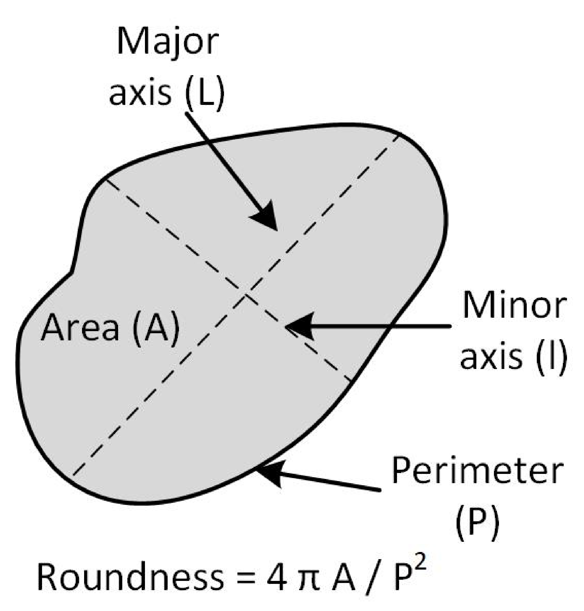
2.3. Data Extraction

Each previously labeled element was manually divided into cells and intercellular spaces, creating two subset folders of images. Next, morphological features were obtained according to Mayor et al. [14] and were selected four of these following the recommendations of Oblitas et al. [9], which determined the optimal parameters of an RBNN for discrimination of microstructural elements in Cucurbita pepo L. tissue using an exhaustive search algorithm. Figure 3 illustrates the selected morphological features.
The obtained feature values were then used in the design, implementation, and analysis of RBNN-based models. Each element in both subsets was resized to 277 × 277 pixels to be used in CNN.

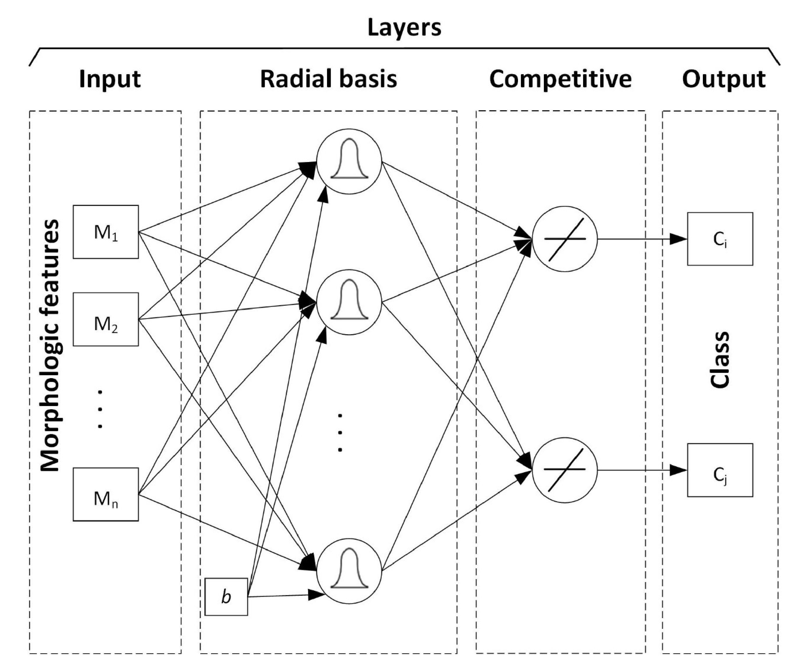
2.4. Radial Basis Neural Network—RBNN

According to Oblitas et al. [9], Artificial Neural Networks (ANN) were inspired by the human nervous system, and they combine the complexity of statistical techniques with self-learning, imitating the human cognitive process. A general scheme for ANNs is shown in Figure 4.
At this point, it is possible to understand that ANNs contain a very complicated set of interdependence and may incorporate some degree of nonlinearity, which helps them to face nonlinear problems.
Likewise, a special kind of ANN named Radial Basis Neural Network (RBNN), which is a specialized feed-forward network for classification, is presented. The principal characteristics of RBNN are that the design parameter is the spread of the radial basis transfer function and that little training is required (except for spread optimization) [21,22].
The RBNN general structure is shown in Figure 5 was used. The first layer computes distances from the input vector to the training input vectors and produces a vector whose elements indicate how close the input is to a training input. The second layer sums these contributions for each class of inputs to produce a vector of probabilities as its net output. Finally, a competitive output layer picks the maximum of these probabilities and produces a 1 for that class and a 0 for the other classes.

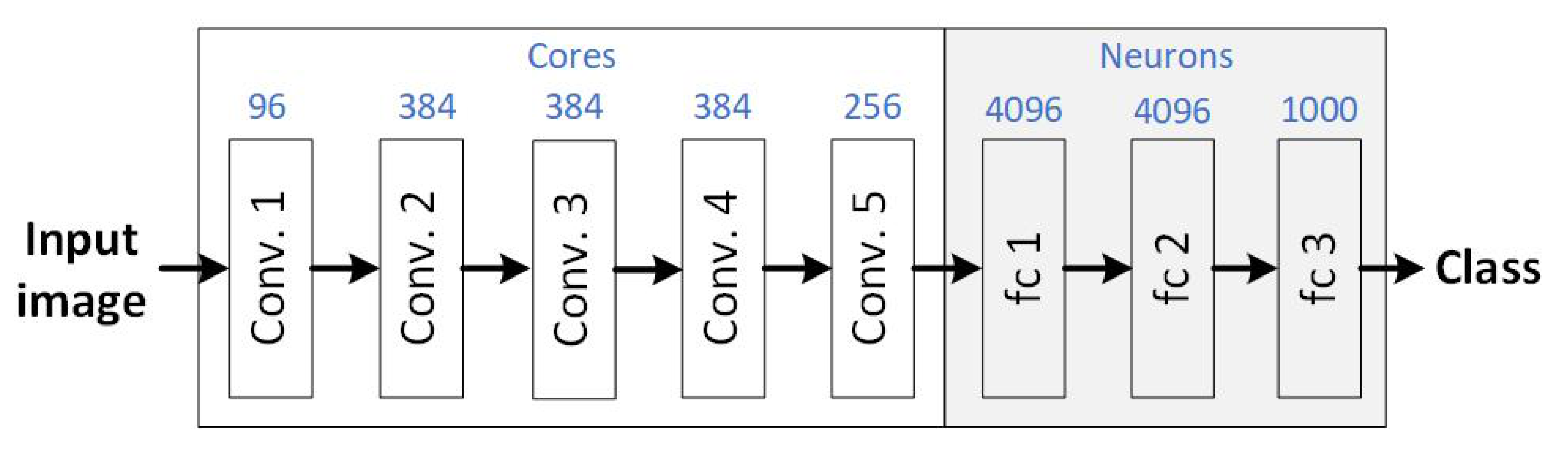
2.5. Convolutional Neural Network—CNN

The CNN AlexNet was used in this study, whose general structure is shown in Figure 6. The AlexNet has five convolutional layers and three fully connected layers. Each convolved layer contains multiple 3D filters (cores) connected to the previous layer’s output. Fully connected layers contain multiple neurons, with positive values, connected to the previous layer [23].
AlexNet was selected because it is one of the most well-known and widely used convolutional neural network architectures for image classification. Besides, a model of AlexNet is provided in MatLab that is trained on more than one million images and can classify objects in up to 1000 categories [24].

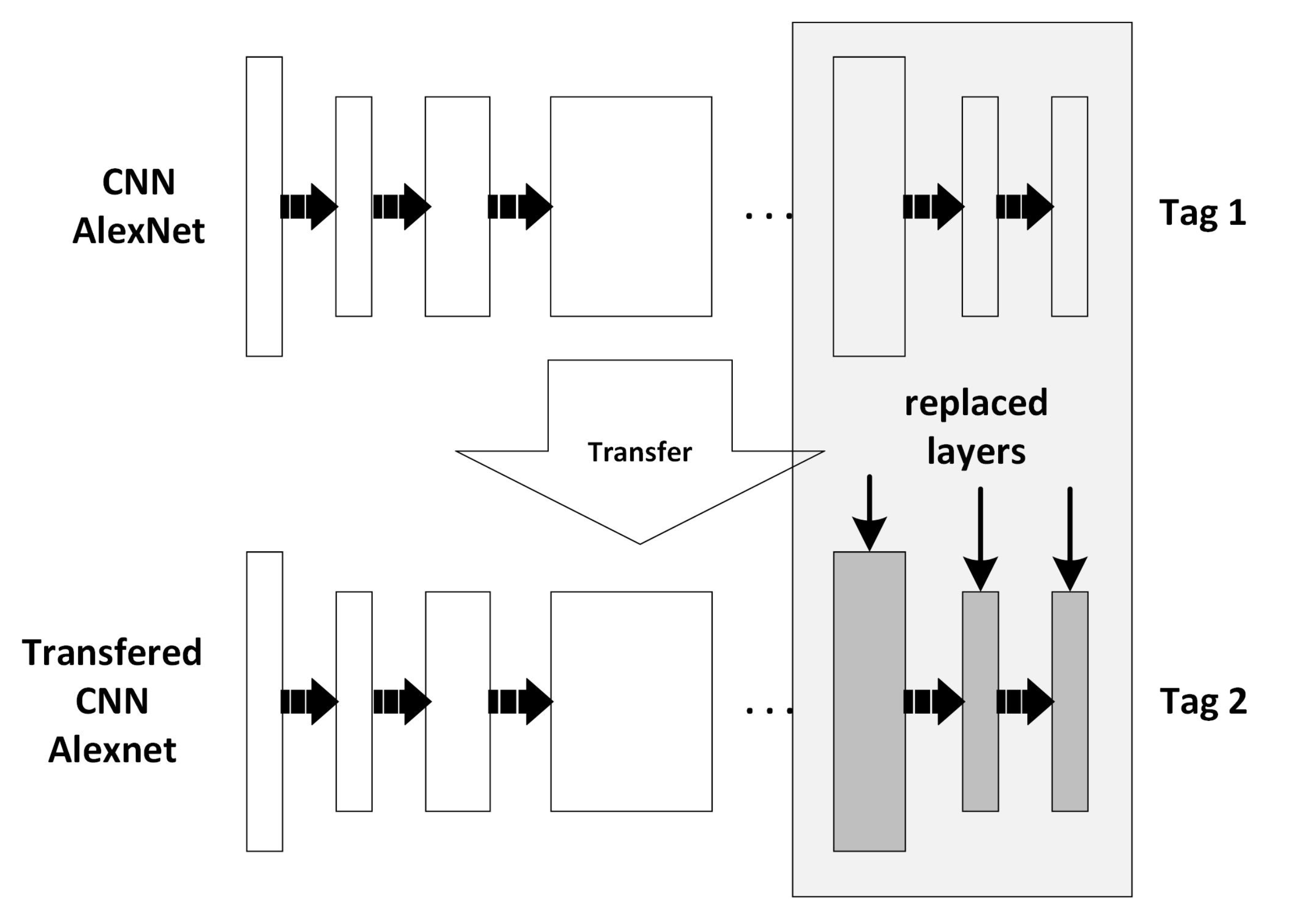
2.6. Learning Transfer

The AlexNet, which is preloaded in Matlab 2018a, was modified to use the previously trained design, similar to that carried out by Zhou et al. [23] and Lu et al. [25]. Essentially, the parameters of the last three layers were modified to transfer the training of the remaining layers and adapt them to the classification process of the previously established classes, see Figure 7.

2.7. Statistical Comparison of Models

The cells and intercellular spaces were randomly divided into five groups. These groups were then used to model, test, and validate the models based on CNN in k-fold cross-validation with k = 5 . For the RBNN-based model, the features and parameters for microstructural elements were obtained according to Section 2.2.2; likewise, as for CNN models, k-fold cross-validation was implemented.
This process was repeated one hundred times to evaluate the robustness of the method, calculating for this purpose, the confusion matrices; Figure 8 shows the basic form of the confusion matrix for binary classification.
A confusion matrix is one of the most commonly used techniques in the machine learning community and contains information about the actual and predicted ratings obtained by a classification system. A confusion matrix has two dimensions: real and predicted classes. Each row represents the instances of a real class, whereas each column represents the cases of a predicted class. In the case of a binary classification, each cells contains: T P (True Positive), correctly identified; T N (True Negative), correctly rejected; F P (False Positive), incorrectly identified; and F N (False Negative), incorrectly rejected.
Some performance measures can be defined from the information contained in a confusion matrix, among them precision, recall, accuracy, and f-measure. These measures are determined by the number of classification errors and hits made by the classifier, as expressed by Equations (7)–(10).
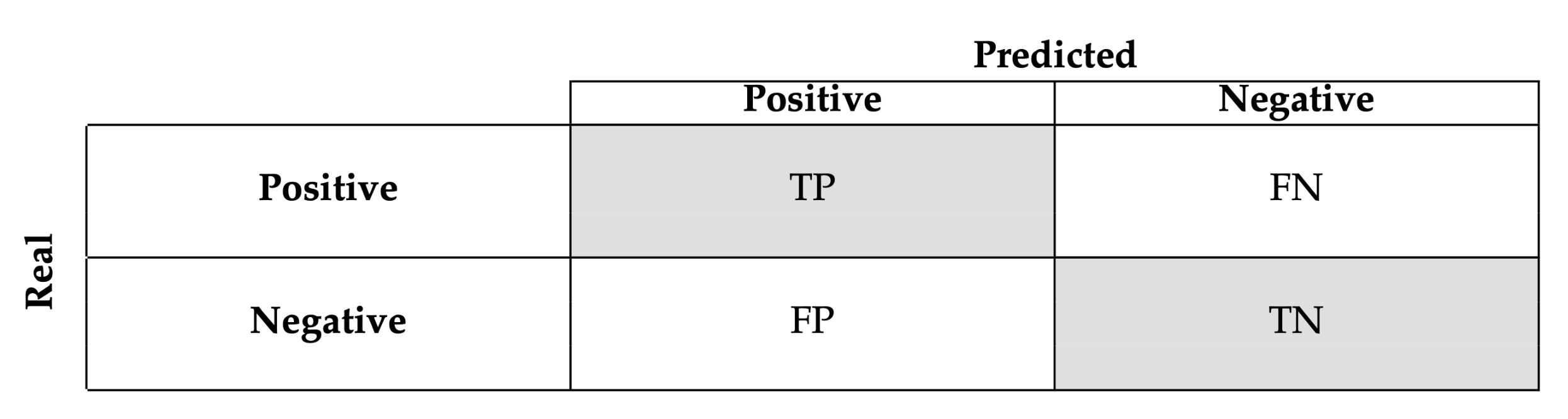
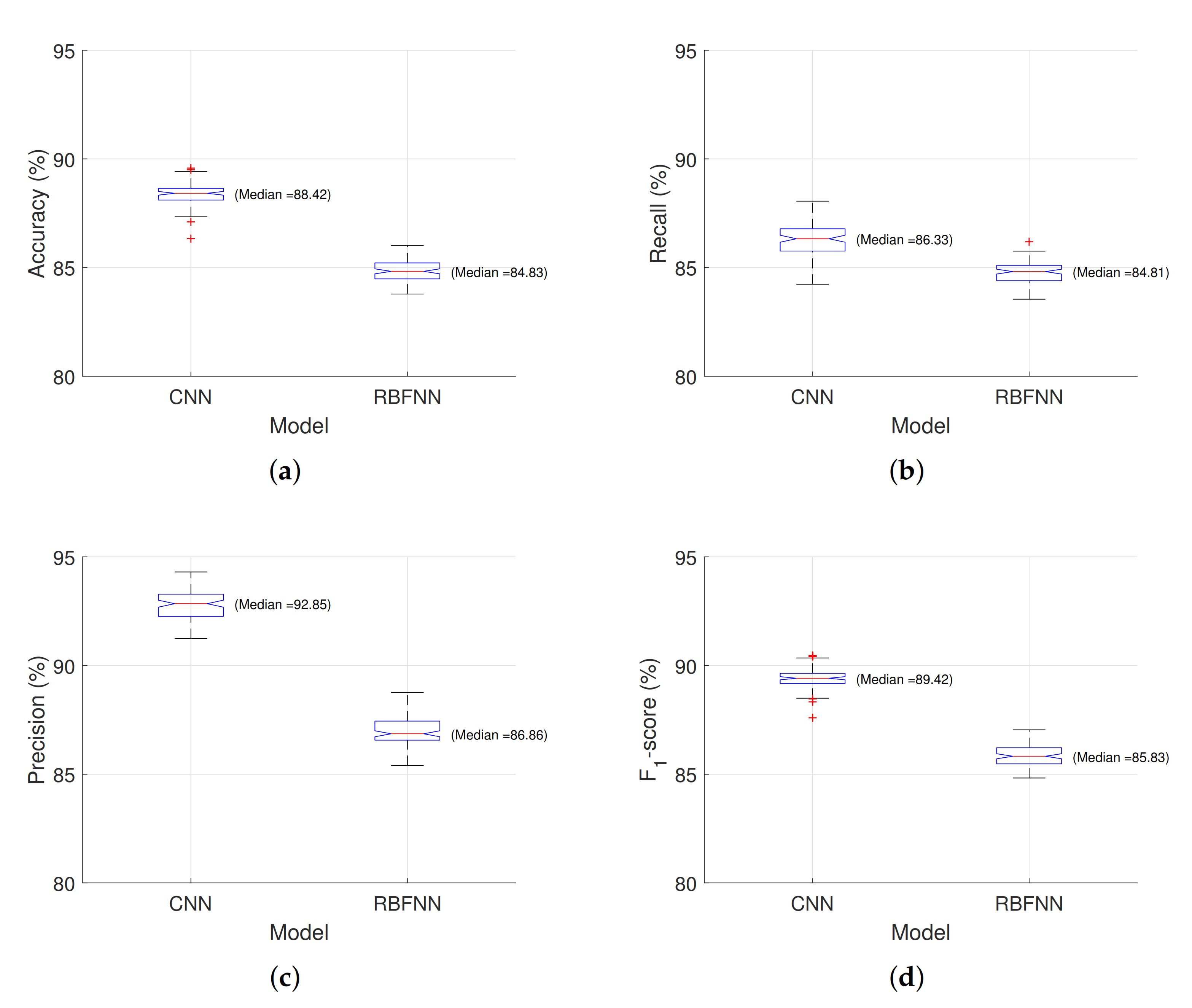
  • Accuracy: This measures how many observations, both positive and negative, were correctly classified and it is defined by Equation (7).
    A c c u r a c y = T P + T N T P + T N + F P + F N
  • Recall: This measures how many observations out of all of the positive observations were classified as positive (see Equation (8)).
    R e c a l l = T P T P + F N
  • Precision: This measures how many observations predicted as positive are, in fact, positive (see Equation (9)).
    P r e c i s i o n = T P T P + F P
  • F1–score: This combines precision and recall into one metric (harmonic mean, see Equation (10)).
    F 1 s c o r e = 2 × P r e c i s i o n × R e c a l l P r e c i s i o n + R e c a l l

3. Results and Discussions

3.1. Digital Micrograph Processing

Figure 9 shows part of an initial micrograph Figure 9a. Likewise, the images resulting from applying the enhancement Figure 9b, skeletonized Figure 9c, and labeling Figure 9d functions. The final image of this process Figure 9d is used in the manual classification process. Consequently, it is necessary to properly extract the elements present in the figure while avoiding losing information to use in the next steps.
The images obtained from the pre-processing step were good enough for visual identification of cellular structures. However, some parameters may be adapted (or optimized) to maximize the information extracted from each micrography due to differences in capture conditions. The processing parameters to be tuned include the type of pre-processing filter, the size of the convolution mask, and the filtering repetitions, among others.

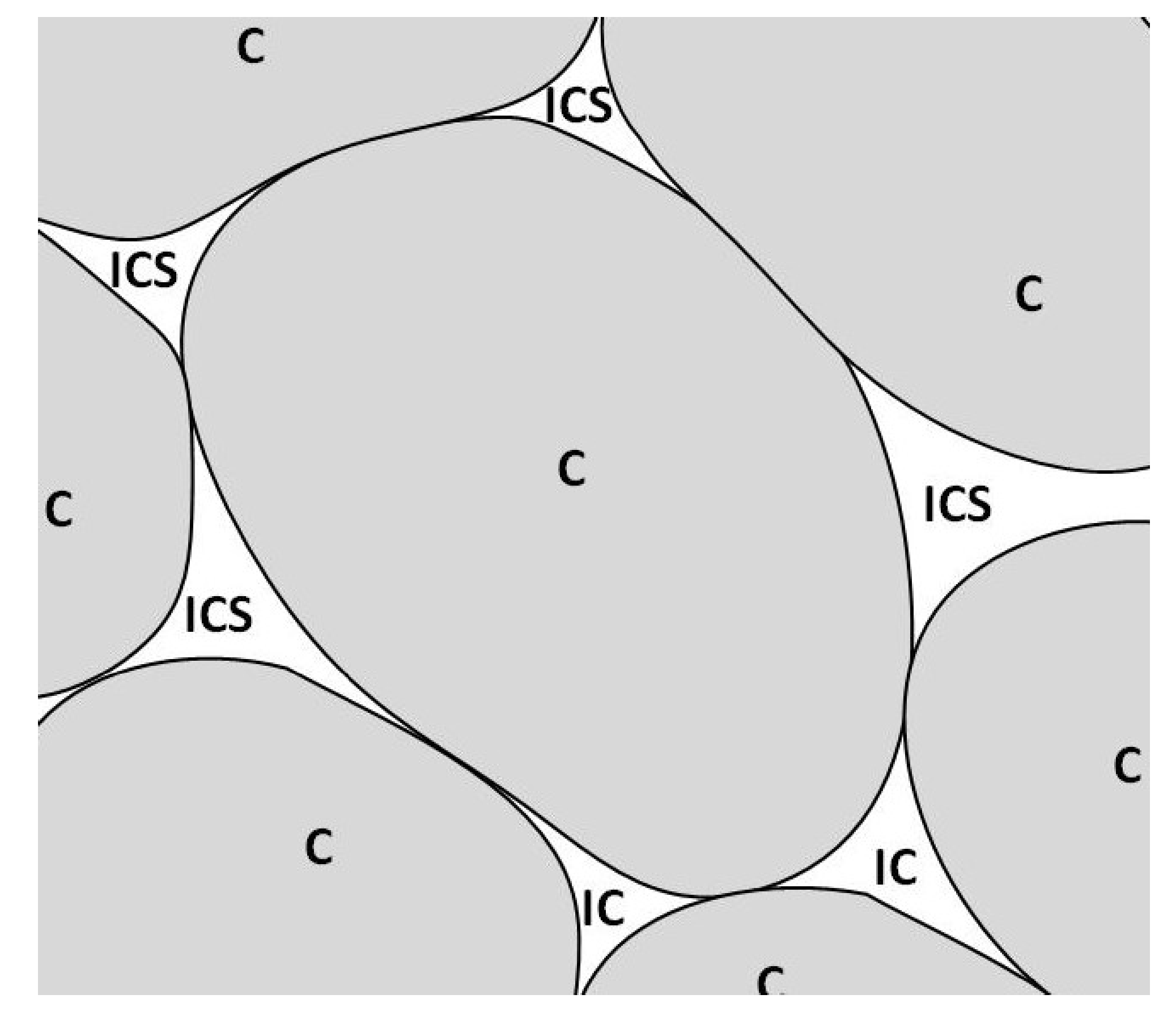
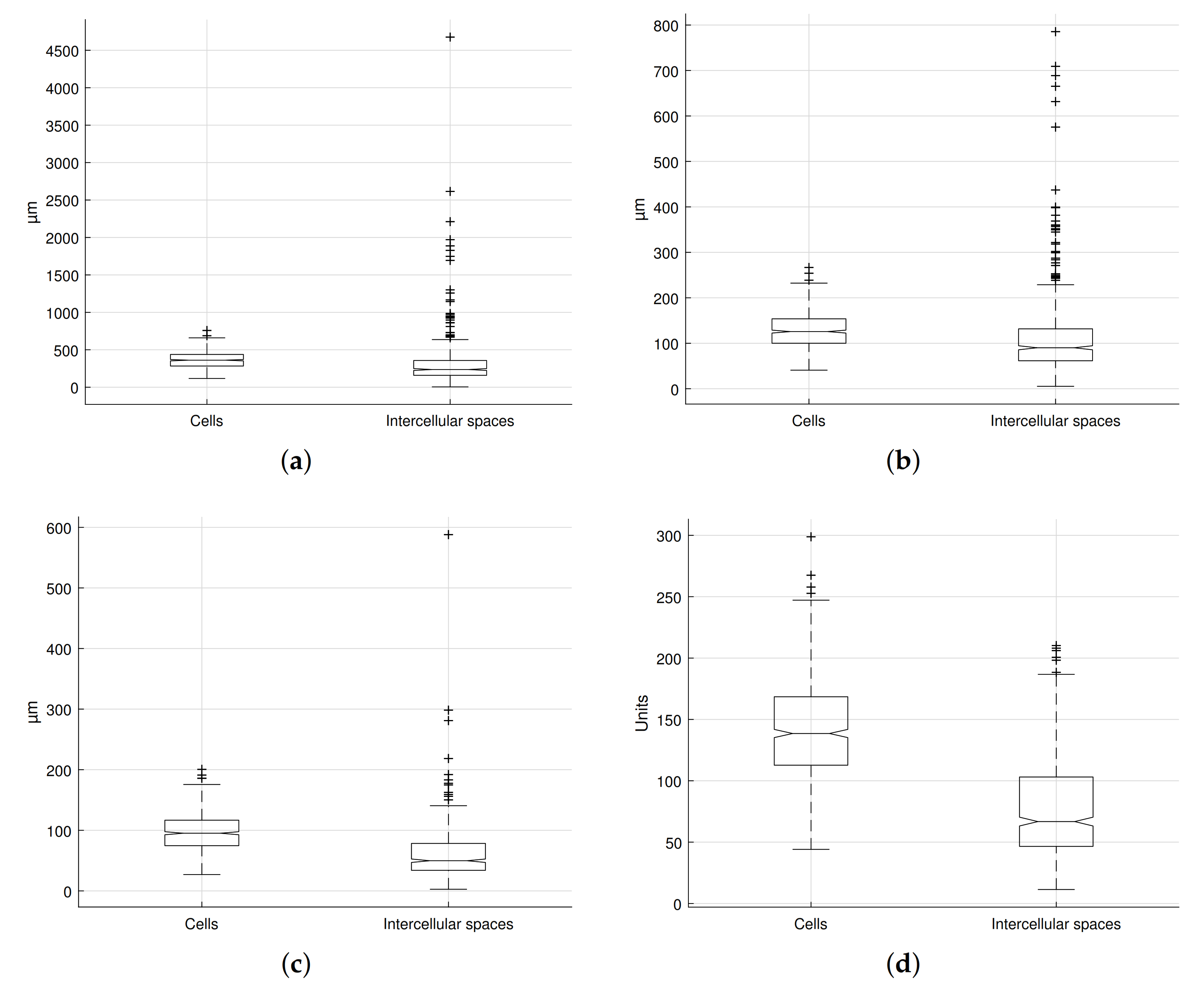
3.2. Microstructural Elements

Figure 10a,b show examples of manually classified structural elements. There were 685 cells and 610 intercellular spaces. Although the number of elements to be used for training and validation of neural network-based models is small, compared to those used by Pieczywek and Zdunek [6], and Kraus et al. [26], it is sufficient to assess its viability for the discrimination of microstructures in vegetal tissue.
Images in Figure 10 evidence that the manual classification is based on morphogeometric features; however, the irregular geometry of the intercellular spaces and the image quality make pre-processing difficult (enhancement and improvement). Consequently, it is not easy to recognize the elements in the image [27,28]. Therefore, it is understandable that there are differences with other methods of determining characteristics, such as those based on manual segmentation with software such as image-J (National Institutes of Mental Health, Bethesda, Maryland, USA) or Adobe Photoshop (Adobe Systems Inc., San José, CA, USA).
Figure 11 shows the values for the selected features according to their manual classification in cells and intercellular spaces. It is observed that there is an overlap in the range covered by the selected morphogeometric characteristics of both microstructural elements. In contrast, the medians and the first two quartiles differ in all cases, especially in the perimeter, length of the minor axis, and roundness.
These differences allow their use for classification with different techniques, such as in the works of Pieczywek and Zdunek [6] using Bayesian Networks or Oblitas et al. [9] with Probabilistic Neural Networks.

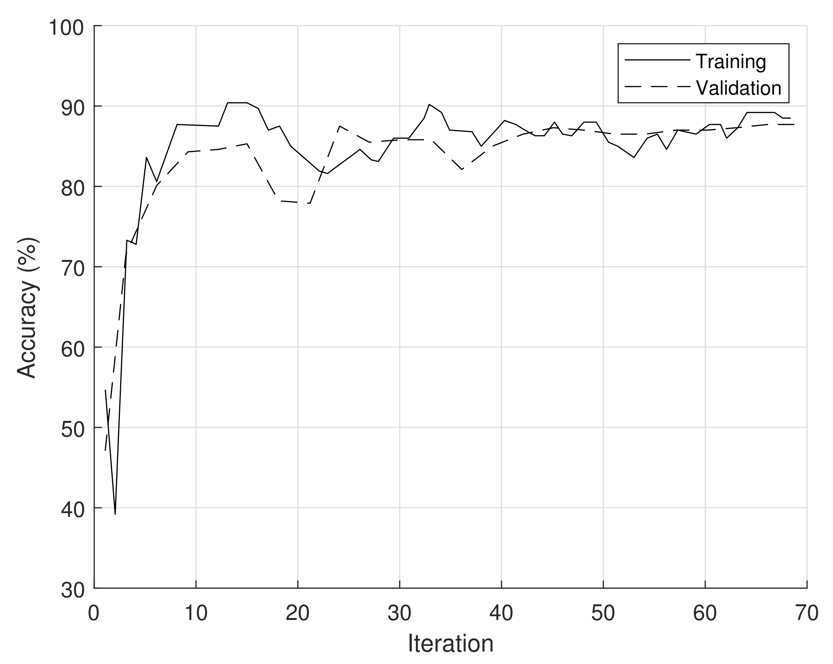
3.3. CNN Implementation

Figure 12 presents the accuracy of the CNN training process in one of the one hundred averaged iterations to determine the system’s accuracy.
As can be seen, the validation reaches stable accuracy values from the third iteration of around 87%. As mentioned by Baker et al. [29], this is possible because the CNN (when they exclusively use the silhouette of objects, preventing textures) tends to be more error-prone.

3.4. Statistical Analysis

The statistical measures obtained for the CNN and RBNN based classification models are shown in Figure 13. As can be seen, except for Recall, both medium and range values were better for CNNs.
The median F1–score obtained in our experiment were 89.42% and 85.43% for CNN and RBNN models, respectively. However, comparing the adjust with those obtained by Pieczywek and Zdunek [6], over 97%, are relatively lower, which could be due to fewer differences between elements in Cucurbita pepo L. in front of Malus Domestica Borkh, mainly expressed in their angularity and roundness.
The classification capacity of both models (CNN and RBNN) was compared through the Accuracy, Recall, Precision, and F1–score indicators. The results, Table 1, show that using CNN gives a higher performance in terms of the four indicators mentioned. When performing the t-test, it was found that the p-value is less than 0.05, which shows that there is a statistically significant difference between the means of both models.
The significant superiority in the CNN’s performance reflects its ability to encode classification information in the internal layers, which it does not share with the RBNN structure. Similarly, when comparing the standard deviation of performance in terms of F1–score, both classifiers have similar stability, with a reduced variation between the one hundred different iterations performed using the k-fold cross-validation strategy. This stability is indicative of the generalization capacity of both models.
Although the CNN AlexNet allows us to classify using two totally connected layers and the softmax function, some works have improved the adjustment by employing a classifier coupled to the CNN, such as the works of Rohmatillah et al. [30], Sadanandan et al. [31], or they have created specific CNN architectures. However, this requires a much more extensive database for training, such as in the works of Sharma et al. [32], Song et al. [33], and Akram et al. [34], among others. In this sense, new studies should be carried on to test this in microstructural element discrimination in vegetal origin food.

4. Conclusions

This work proposed the use of machine learning techniques to discriminate microstructural elements in vegetal tissues; this is the first report of the use of CNN to discriminate microstructural elements in vegetal origin food. As a case study, the microstructures of Cucurbita pepo L. tissue were classified. The CNN and RBNN techniques were compared to evaluate differences in performance measures derived from the confusion matrix. Results show that both methods produce relatively good discrimination when compared with other studies, with a median F1–score of 89.42% and 85.43% for CNN and RBNN, respectively. However, the CNN presented a consistent and significantly higher. Likewise, in terms of stability, a reduced variation is obtained and evaluated by the F-test. This indicates that both models have good generalization capacity. Consequently, the use of the CNN technique shows the potential for microstructural element discrimination in the tissue of vegetal origin and better conditions in front of RBNN.
For future works it is considered to analyze the effect of different architectures of convolutional networks (number and size of layers, filters and discrimination functions) to be used in processes of discrimination of cellular structures or similar tasks. Finally, tissue structures from other vegetables may be analyzed to find the utility of the proposed method in different applications.

Author Contributions

Conceptualization, L.M.L., J.O. and W.C.; methodology, W.C. and J.O.; software, W.C. and M.D.-l.-T.; validation, L.S.G., L.M.L., A.I. and J.M.; formal analysis, W.C., M.D.-l.-T. and H.A.-G.; resources, L.S.G., L.M.L. and W.C.; data curation, H.A.-G. and M.D.-l.-T.; writing—original draft preparation, J.O., W.C. and H.A.-G.; writing—review and editing, M.D.-l.-T., H.A.-G., J.M., and W.C.; visualization, W.C. and M.D.-l.-T.; supervision, L.S.G., L.M.L. and A.I.; project administration, H.A.-G.; funding acquisition, W.C. All authors have read and agreed to the published version of the manuscript.

Funding

This research received no external funding.

Institutional Review Board Statement

Not applicable.

Informed Consent Statement

Not applicable.

Conflicts of Interest

The authors declare no conflict of interest.

References

  1. Betoret, E.; Betoret, N.; Rocculi, P.; Dalla Rosa, M. Strategies to improve food functionality: Structure–property relationships on high pressures homogenization, vacuum impregnation and drying technologies. Trends Food Sci. Technol. 2015, 46, 1–12. [Google Scholar] [CrossRef]
  2. Fito, P.; LeMaguer, M.; Betoret, N.; Fito, P.J. Advanced food process engineering to model real foods and processes: The SAFES methodology. J. Food Eng. 2007, 83, 173–185. [Google Scholar] [CrossRef]
  3. Topete-Betancourt, A.; Figueroa-Cárdenas, J.d.D.; Morales-Sánchez, E.; Arámbula-Villa, G.; Pérez-Robles, J.F. Evaluation of the mechanism of oil uptake and water loss during deep-fat frying of tortilla chips. Rev. Mex. Ing. QuíMica 2020, 19, 409–422. [Google Scholar] [CrossRef] [Green Version]
  4. Silva-Jara, J.M.; López-Cruz, R.; Ragazzo-Sánchez, J.A.; Calderón-Santoyo, M. Antagonistic microorganisms efficiency to suppress damage caused by Colletotrichum gloeosporioides in papaya crop: Perspectives and challenges. Rev. Mex. Ing. QuíMica 2020, 19, 839–849. [Google Scholar] [CrossRef]
  5. Aguilera, J.M. Why food microstructure? J. Food Eng. 2005, 67, 3–11. [Google Scholar] [CrossRef]
  6. Pieczywek, P.; Zdunek, A. Automatic classification of cells and intercellular spaces of apple tissue. Comput. Electron. Agric. 2012, 81, 72–78. [Google Scholar] [CrossRef]
  7. Mayor, L.; Pissarra, J.; Sereno, A.M. Microstructural changes during osmotic dehydration of parenchymatic pumpkin tissue. J. Food Eng. 2008, 85, 326–339. [Google Scholar] [CrossRef]
  8. Mebatsion, H.; Verboven, P.; Verlinden, B.; Ho, Q.; Nguyen, T.; Nicolaï, B. Microscale modelling of fruit tissue using Voronoi tessellations. Comput. Electron. Agric. 2006, 52, 36–48. [Google Scholar] [CrossRef]
  9. Oblitas, J.; Castro, W.; Mayor, L. Effect of different combinations of size and shape parameters in the percentage error of classification of structural elements in vegetal tissue of the pumpkin Cucurbita pepo L. using probabilistic neural networks. Rev. Fac. Ing. Univ. Antioq. 2016, 30–37. [Google Scholar] [CrossRef]
  10. Meng, N.; Lam, E.; Tsia, K.; So, H. Large-scale multi-class image-based cell classification with deep learning. IEEE J. Biomed. Health Inform. 2018, 23. [Google Scholar] [CrossRef]
  11. Adeshina, S.; Adedigba, A.; Adeniyi, A.; Aibinu, A. Breast Cancer Histopathology Image Classification with Deep Convolutional Neural Networks. In Proceedings of the IEEE 14th International Conference on Electronics Computer and Computation, Kaskelen, Kazakhstan, 29 Novermber–1 December 2018; pp. 206–212. [Google Scholar] [CrossRef]
  12. Aliyu, H.; Sudirman, R.; Razak, M.; Wahab, M. Red Blood Cell Classification: Deep Learning Architecture Versus Support Vector Machine. In Proceedings of the IEEE 2nd International Conference on BioSignal Analysis, Processing and Systems, Kuching, Malaysia, 24–26 July 2018; pp. 142–147. [Google Scholar] [CrossRef]
  13. Reddy, A.; Juliet, D. Transfer Learning with ResNet-50 for Malaria Cell-Image Classification. In Proceedings of the IEEE International Conference on Communication and Signal Processing, Weihai, China, 28–30 September 2019; pp. 945–949. [Google Scholar] [CrossRef]
  14. Mayor, L.; Moreira, R.; Sereno, A. Shrinkage, density, porosity and shape changes during dehydration of pumpkin (Cucurbita pepo L.) fruits. J. Food Eng. 2011, 103, 29–37. [Google Scholar] [CrossRef]
  15. Castro, W.; Oblitas, J.; De-La-Torre, M.; Cotrina, C.; Bazán, K.; Avila-George, H. Classification of cape gooseberry fruit according to its level of ripeness using machine learning techniques and different color spaces. IEEE Access 2019, 7, 27389–27400. [Google Scholar] [CrossRef]
  16. Valdez-Morones, T.; Pérez-Espinosa, H.; Avila-George, H.; Oblitas, J.; Castro, W. An Android App for detecting damage on tobacco (Nicotiana tabacum L) leaves caused by blue mold (Penospora tabacina Adam). In Proceedings of the 2018 7th International Conference On Software Process Improvement (CIMPS), Jalisco, Mexico, 17–19 October 2018; pp. 125–129. [Google Scholar] [CrossRef]
  17. Castro, W.; Oblitas, J.; Chuquizuta, T.; Avila-George, H. Application of image analysis to optimization of the bread-making process based on the acceptability of the crust color. J. Cereal Sci. 2017, 74, 194–199. [Google Scholar] [CrossRef]
  18. De-la Torre, M.; Zatarain, O.; Avila-George, H.; Muñoz, M.; Oblitas, J.; Lozada, R.; Mejía, J.; Castro, W. Multivariate Analysis and Machine Learning for Ripeness Classification of Cape Gooseberry Fruits. Processes 2019, 7, 928. [Google Scholar] [CrossRef] [Green Version]
  19. Saha, P.; Borgefors, G.; di Baja, G. Skeletonization: Theory, Methods and Applications; Academic Press: Cambridge, MA, USA, 2017. [Google Scholar]
  20. González, R.; Woods, R.; Eddins, S. Digital Image Processing Using MATLAB; Pearson Education: Chennai, India, 2004. [Google Scholar]
  21. Fernández-Navarro, F.; Hervás-Martínez, C.; Gutiérrez, P.; Carbonero-Ruz, M. Evolutionary q-Gaussian radial basis function neural networks for multiclassification. Neural Netw. 2011, 24, 779–784. [Google Scholar] [CrossRef]
  22. Huang, W.; Oh, S.; Pedrycz, W. Design of hybrid radial basis function neural networks (HRBFNNs) realized with the aid of hybridization of fuzzy clustering method (FCM) and polynomial neural networks (PNNs). Neural Netw. 2014, 60, 166–181. [Google Scholar] [CrossRef] [PubMed]
  23. Zhou, Y.; Nejati, H.; Do, T.; Cheung, N.; Cheah, L. Image-based vehicle analysis using deep neural network: A systematic study. In Proceedings of the IEEE International Conference on Digital Signal Processing, Beijing, China, 16–18 October 2016; pp. 276–280. [Google Scholar] [CrossRef] [Green Version]
  24. Toliupa, S.; Tereikovskyi, I.; Tereikovskyi, O.; Tereikovska, L.; Nakonechnyi, V.; Kulakov, Y. Keyboard Dynamic Analysis by Alexnet Type Neural Network. In Proceedings of the 2020 IEEE 15th International Conference on Advanced Trends in Radioelectronics, Telecommunications and Computer Engineering (TCSET), Lviv-Slavske, Ukraine, 25–29 February 2020; pp. 416–420. [Google Scholar] [CrossRef]
  25. Lu, S.; Lu, Z.; Zhang, Y. Pathological brain detection based on AlexNet and transfer learning. J. Comput. Sci. 2019, 30, 41–47. [Google Scholar] [CrossRef]
  26. Kraus, O.; Ba, J.; Frey, B. Classifying and segmenting microscopy images with deep multiple instance learning. Bioinformatics 2016, 32, i52–i59. [Google Scholar] [CrossRef] [PubMed]
  27. Du, C.; Sun, D. Learning techniques used in computer vision for food quality evaluation: A review. J. Food Eng. 2006, 72, 39–55. [Google Scholar] [CrossRef]
  28. Brosnan, T.; Sun, D. Improving quality inspection of food products by computer vision—A review. J. Food Eng. 2004, 61, 3–16. [Google Scholar] [CrossRef]
  29. Baker, N.; Lu, H.; Erlikhman, G.; Kellman, P. Deep convolutional networks do not classify based on global object shape. PLoS Comput. Biol. 2018, 14, e1006613. [Google Scholar] [CrossRef] [PubMed] [Green Version]
  30. Rohmatillah, M.; Pramono, S.; Suyono, H.; Sena, S. Automatic Cervical Cell Classification Using Features Extracted by Convolutional Neural Network. In Proceedings of the IEEE 2018 Electrical Power, Electronics, Communications, Controls and Informatics Seminar (EECCIS), Batu, Indonesia, 9–11 October 2018; pp. 382–386. [Google Scholar] [CrossRef]
  31. Sadanandan, S.; Ranefall, P.; Wählby, C. Feature augmented deep neural networks for segmentation of cells. In Proceedings of the European Conference on Computer Vision, Amsterdam, The Netherlands, 8–16 October 2016; pp. 231–243. [Google Scholar] [CrossRef]
  32. Sharma, M.; Bhave, A.; Janghel, R. White Blood Cell Classification Using Convolutional Neural Network. In Soft Computing and Signal Processing; Springer: Berlin, Germany, 2019; pp. 135–143. [Google Scholar] [CrossRef]
  33. Song, W.; Li, S.; Liu, J.; Qin, H.; Zhang, B.; Zhang, S.; Hao, A. Multitask Cascade Convolution Neural Networks for Automatic Thyroid Nodule Detection and Recognition. IEEE J. Biomed. Health Inform. 2018, 23, 1215–1224. [Google Scholar] [CrossRef] [PubMed]
  34. Akram, S.; Kannala, J.; Eklund, L.; Heikkilä, J. Cell proposal network for microscopy image analysis. In Proceedings of the 2016 IEEE International Conference on Image Processing (ICIP), Phoenix, AZ, USA, 25–28 September 2016; pp. 3199–3203. [Google Scholar] [CrossRef]
Figure 1. Relationships in process conditions, as well as food structure and property.
Applsci 11 01581 g001
Figure 2. Representation of cells (C) and intercellular spaces (ICS) in vegetal tissue.
Applsci 11 01581 g002
Figure 3. Morphological features in the segmented microstructural element.
Applsci 11 01581 g003
Figure 4. General scheme for Artificial Neural Network (ANN).
Applsci 11 01581 g004
Figure 5. Architecture of Radial Basis Neural Network (RBNN).
Applsci 11 01581 g005
Figure 6. General scheme of the AlexNet application.
Applsci 11 01581 g006
Figure 7. Learning transfer for Convolutional Neural Network (CNN) AlextNet.
Applsci 11 01581 g007
Figure 8. Example of confusion matrix for binary classification.
Applsci 11 01581 g008
Figure 9. Results of micrograph processing: (a) initial, (b) enhanced, (c) skeletonized, and (d) labeling.
Applsci 11 01581 g009
Figure 10. Images of microstructural elements: (a) cells and (b) intercellular spaces.
Applsci 11 01581 g010
Figure 11. Selected feature values for microstructural elements in the studied sample: (a) perimeter, (b) length of mayor axis, (c) length of minor axis, and (d) roundness.
Applsci 11 01581 g011
Figure 12. Accuracy during CNN training.
Applsci 11 01581 g012
Figure 13. Performing measures for CNN and RBNN based classifier: (a) perimeter, (b) length of mayor axis, (c) length of minor axis, and (d) roundness.
Applsci 11 01581 g013
Table 1. Statistics for the comparison of the models.
Comparison Performance Measure
AccuracyRecallPrecision F 1 Score
Meanst-test−47.4999−25.9556−36.9701−14.8146
p-value0000
Standard deviationF-test0.50360.64532.07891.2957
p-value0.00070.03040.00030.1992
Publisher’s Note: MDPI stays neutral with regard to jurisdictional claims in published maps and institutional affiliations.

