A Biologically Inspired Sound Localisation System Using a Silicon Cochlea Pair

Abstract

We present a biologically inspired sound localisation system for reverberant environments using the Cascade of Asymmetric Resonators with Fast-Acting Compression (CAR-FAC) cochlear model. The system exploits a CAR-FAC pair to pre-process binaural signals that travel through the inherent delay line of the cascade structures, as each filter acts as a delay unit. Following the filtering, each cochlear channel is cross-correlated with all the channels of the other cochlea using a quantised instantaneous correlation function to form a 2-D instantaneous correlation matrix (correlogram). The correlogram contains both interaural time difference and spectral information. The generated correlograms are analysed using a regression neural network for localisation. We investigate the effect of the CAR-FAC nonlinearity on the system performance by comparing it with a CAR only version. To verify that the CAR/CAR-FAC and the quantised instantaneous correlation provide a suitable basis with which to perform sound localisation tasks, a linear regression, an extreme learning machine, and a convolutional neural network are trained to learn the azimuthal angle of the sound source from the correlogram. The system is evaluated using speech data recorded in a reverberant environment. We compare the performance of the linear CAR and nonlinear CAR-FAC models with current sound localisation systems as well as with human performance.

1. Introduction

This work is inspired by the high accuracy and robustness with which the human auditory system perceives sound in cluttered acoustical environments. In the human auditory pathway, binaural signals are pre-processed in the cochlea, transformed into neural signals in the auditory nerve (AN), and transmitted through the cochlear nucleus (CN) to the superior olivary complex (SOC). The interaural time difference (ITD) cues of the binaural signal are believed to be encoded in the medial superior olive (MSO) [1,2]. The neurons in the MSO receive excitation from large spherical bushy cells (SBCs) of the CN in both the ipsilateral and contralateral side and inhibitory from the ipsilateral lateral nucleus of the trapezoid body. The interaural level difference (ILD) cues of the binaural signal are believed to be encoded in the lateral superior olive (LSO) [2,3]. The neurons in the LSO receive excitation from the small SBCs of the ipsilateral CN, and inhibition from the contralateral side relayed through inhibitory neurons in the nucleus of the trapezoid body. The ITD and ILD are the primary cues for sound source localisation according to the “duplex theory of sound localisation” proposed by Rayleigh in Reference [4]. Rayleigh theorised the ITD cues dominate at low frequencies while the ILD cues dominate at high frequencies (in humans, above 2–3 kHz) where the wavelength is short, and the head can act as an acoustic shadow. So far, many psychophysical experiments have shown support for the duplex theory [2,5,6,7,8,9,10,11], and the duplex conception is still a standard idea for how binaural hearing works.

To try to mimic the human auditory system in localising a sound source, biologically inspired sound localisation systems have been proposed and developed. For example, R. F. Lyon [12] proposed a computational model of binaural localisation and separation, in which peaks of short-time cross-correlation functions between each channel of two cochlear models indicate the direction of a sound source; S. A. Shamma et al. [13] proposed a computational model including two cochlear models and a Jeffress delay line [14] to encode the ITD cues. In a study by M. Heckmann et al. [15], both ITD cues from cross-correlation functions and ILD cues were used for echoic and noisy environments.

Although both ITD and ILD cues are involved in human sound localisation horizontally [16], hardware development mainly uses the ITD cue since it is relatively strong and easy to obtain without any additional requirements such as a dummy head or an artificial pinna pair. The first neuromorphic model for auditory localisation was implemented by Lazzaro and Mead [17]. They built the Jeffress model [18] with a cochlear pair on an analogue chip. The system created delay lines from two cochlear channels with a maximum delay value of the maximum ITD expected and a minimum delay value equal to the system resolution. After this, N. Bhadkamkar et al. [19] implemented a two-chip system: One chip for a cochlear pair and the other one for a delay line model. I. Grech et al. [20] built a three-chip system with four microphones to detect the 3-D location of a sound source. In the system, the first chip was for the cochlear pair and ILD extraction, the second chip was for the onset detection, and the third chip was for the ITD extraction. This system showed a root mean square (RMS) error of 5° in azimuth and elevation. However, the hardware implementation of the delay lines makes those systems large. Alternatively, delay lines can be implemented by using the inherent characteristics of the cascade cochlear structure. In a cascade cochlear filter model, each stage of the filter adds a certain delay so that the cascade itself acts as a delay line. The correlations between the two cochlear channels thus encode the ITD cues of a sound source. Such an approach was implemented on an analogue chip in Reference [21]. They presented the formations of the 2-D cochlear correlograms in detail, and it forms the basis of this work. Another way of obtaining ITD cues was proposed by van Schaik and Shamma. They implemented a neuromorphic sound localiser in Reference [22]. In the system, a delay between the positive zero-crossings of both ears was detected, and a pulse was generated with the width equal to the delay value. A voltage across a capacitor, proportional to the average pulse width, was obtained by integrating over a fixed number of pulses. Once a fixed number of pulses was counted, the capacitor was read and reset.

To emulate the robustness of the human sound localisation performance in noisy environments, neural network algorithms are introduced to analyse the ITD cues from cochlear models. Implementations of such auditory “where” pathways have been proposed and developed increasingly [23,24,25,26,27]. For example, K. Iwasa et al. [25] and M. Kugler et al. [26] used a competitive learning network with a pulsed neuron model (CONP) to learn the direction of a sound source. C. Schauer et al. [28] proposed to build a spike-based sound localisation system on Field Programmable Gate Array (FPGA). They used a Leaky Intgrate-and-Fire (LIF) neuron model to generate spikes from a cochlear inner hair cell output, and a delay line to extract ITD cues from the spike streams. A Winner-take-all (WTA) network was then used to select the dominant sound source direction. Chan et al. proposed a robotic sound localisation system using a WTA network to estimate the direction of a sound source through the ITD cues from a cochlea pair with an address event representation (AER) interface [27]. In recent years, deep neural networks (DNN) have provided more accurate estimations of sound source locations from binaural cues [29,30,31,32]. For example, in S. Jiang et al. [32], simulated binaural signals were pre-processed with a Gammatone filter bank and used to train a DNN classifier for sound source localisation. Although some of those systems showed small RMS errors, they used either simulated signals or sinewaves, instead of natural sounds, such as speech signals, as the input signal. The robust performance of biologically inspired sound localisation systems for practical applications are yet to be tested and proved.

In this work, we present a biologically inspired sound localisation system and evaluate its performance for a practical task: speech localisation, in a small office. We propose to use the CAR-FAC cochlear model to generate correlograms and a regression Extreme Learning Machine (ELM) to localise a sound source from the correlograms in Reference [33]. In the human binaural system, a mechanism called the precedence effect is thought to allow suppression of echoes to help localisation between a direct sound and a reflection. The precedence effect refers to the phenomena that we perceive the location of a sound source based on sound onset and ignore the localisation cues that follow from about 2 ms up to 40 ms [34,35]. Inspired by this, we use an onset detection algorithm to generate the correlogram only during the signal onset to decrease the influence of echoes. We then proposed to use a regression convolutional neural network (CNN) for sound localisation in Reference [36]. In this work, we describe the system in detail and investigate the effect of the CAR-FAC nonlinearity on the system performance by comparing it with a CAR only version. The performance of the quantised correlograms is also compared with non-quantised correlograms. The implementation and evaluation of the system will be described in the next sections.

2. Materials and Methods

The top-level structure of the proposed sound location system is shown in Figure 1. A binaural CAR-FAC cochlear system is built to pre-process binaural signals. It includes two CAR-FAC modules, and each cochlear channel is connected to a lateral inhibition (LI) block that models the cochlear nucleus (CN) function. The two CAR-FACs act as delay lines and the LI output from all the channels are compared with each other in parallel using coincidence detection to model the medial superior olive (MSO) function. A sound onset detector is used to detect signal onset so that the correlograms are only generated during the signal onset period to decrease the influence of echoes. The onset correlograms are analysed using a regression convolutional neural network (CNN).

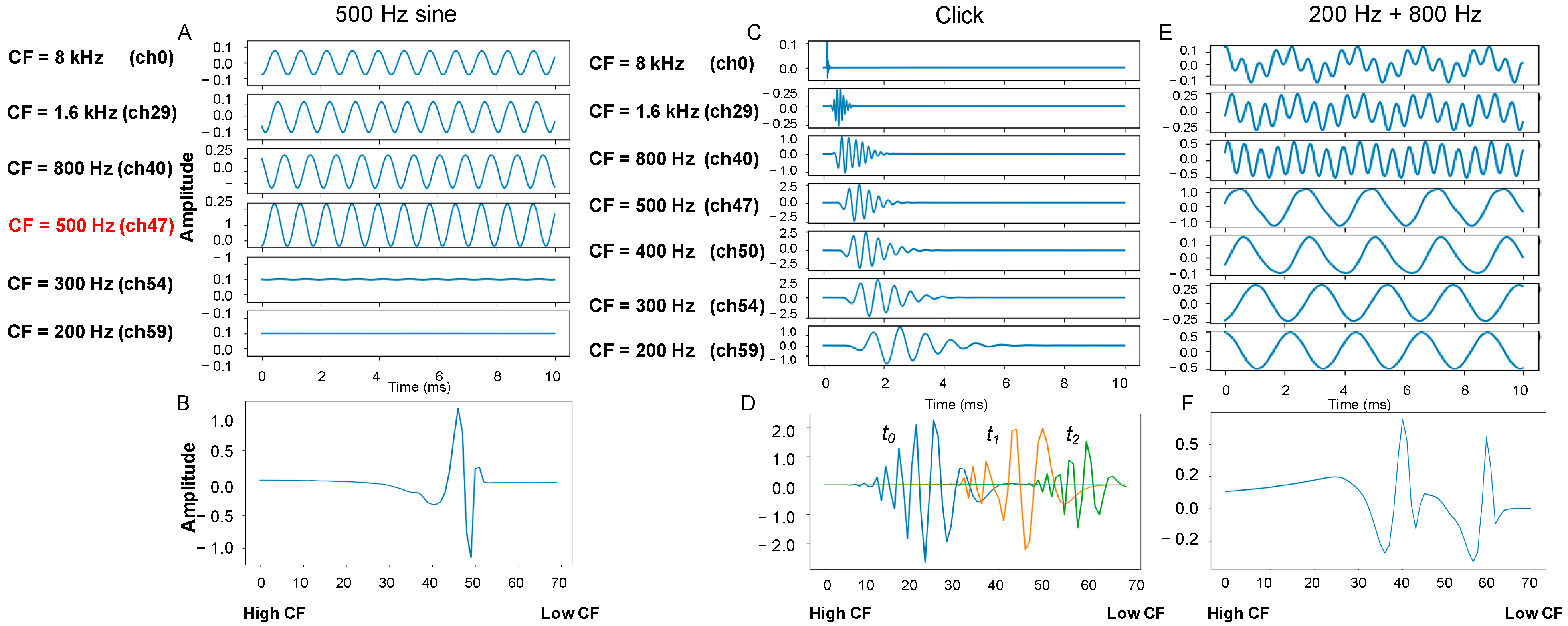
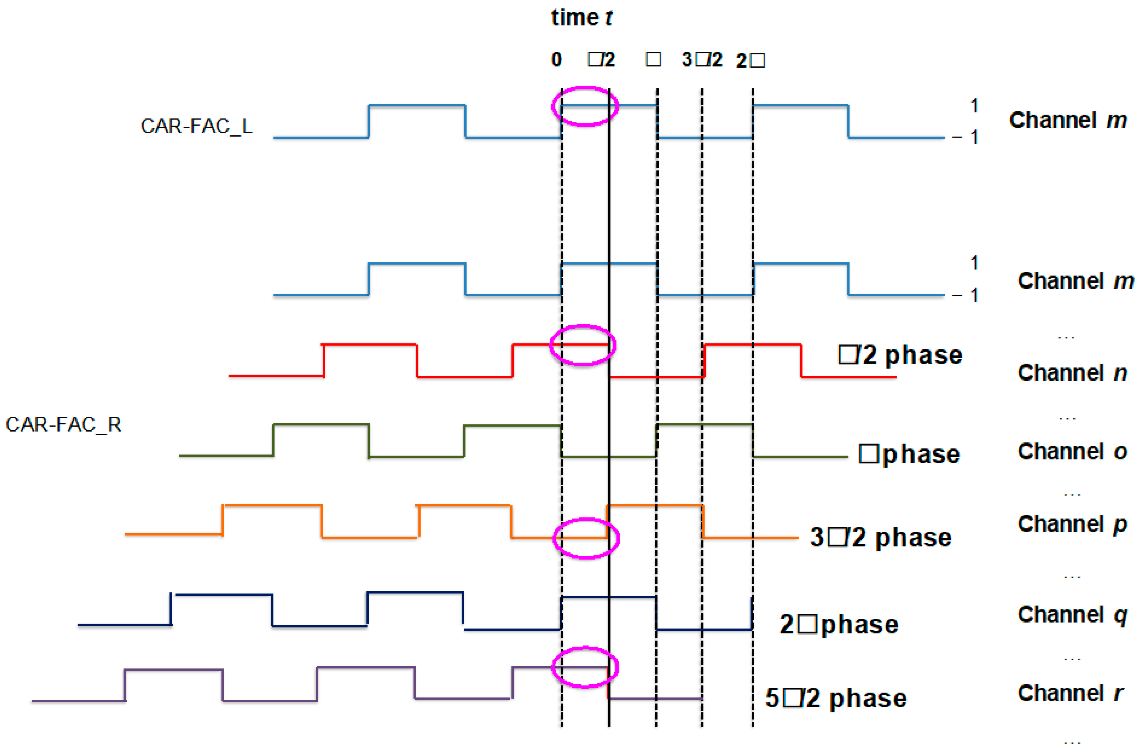
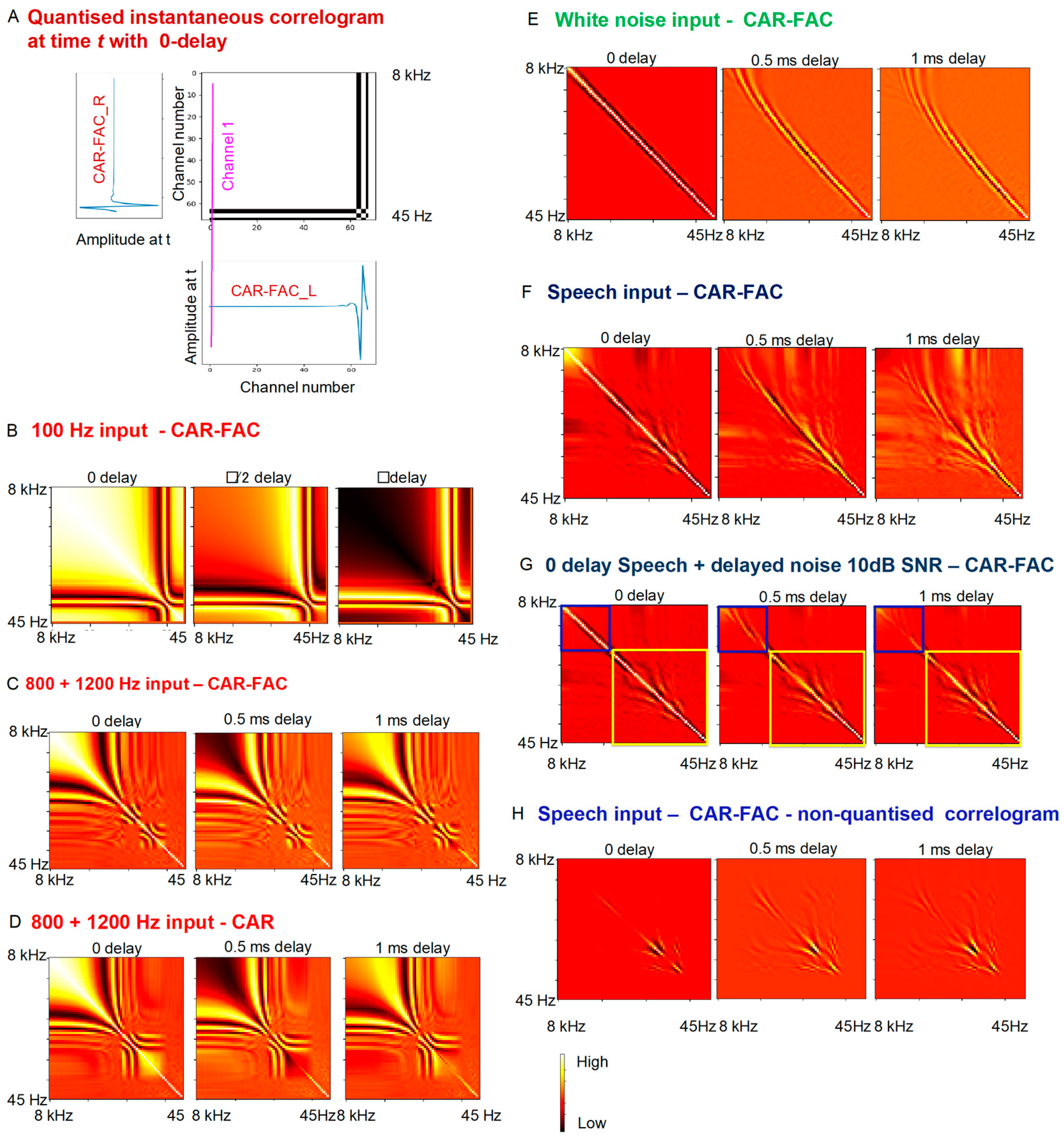
2.1. Binaural CAR-FAC Pre-Processing

The CAR-FAC cochlear model was proposed in Reference [37], and a real-time reconfigurable CAR-FAC implementation on FPGA was described in References [38,39]. As shown in Figure 1A, the CAR models the basilar membrane (BM) function using a cascade of two-pole-two-zero resonators, H₁ to H_N. The poles of the two-pole-two-zero resonator are chosen to be equally spaced along the normalised length of the cochlea according to the Greenwood map function [40]. The FAC includes a digital outer hair cell (DOHC) model, a digital inner hair cell (DIHC) model, and combines local instantaneous nonlinearity with a multi-time-scale automatic gain control (AGC). In this work, to investigate the FAC effect on the system performance, we also use the CAR only as a linear cochlear pre-processing step to compare its performance with the CAR-FAC pre-processing. The details are described in the Results and Discussion section. The lateral inhibition (LI) function models the role of cochlear nucleus neurons. Here, we extend the work to implement a real-time binaural CAR-FAC system on an Altera Cyclone V FPGA board using time multiplexing and pipeline parallelising techniques, as shown in Figure 2. The detailed implementation of each element of the CAR-FAC and the LI is described in References [36,38,39,41,42]. In this work, the LI outputs from both ‘ears’ are used to generate correlogram in the Correlogram module, and the correlogram is the system output. Other choices for the output of the binaural CAR-FAC system include the BM and the DIHC.

The CAR-FAC response forms the basis of this system, Figure 3 presents examples of a 70-channel CAR-FAC response to different input sounds. Figure 3A shows the BM response to a 500 Hz sine tone at six channels, and Figure 3B shows the BM spatial response across all the channels at time t. At higher centre frequency (CF) channels, the 500 Hz waveform travels without significant gain, and the output shows a gradually increased gain across those channels. As the waveform reaches the 500 Hz CF channel, a maximum gain is shown. After this, the gain of the response reduces rapidly. Figure 3C shows the BM response of seven channels to a “click”. The click is a short period broadband signal so that each channel effectively shows its impulse response, and the dominant response frequency corresponds to each channel’s CF. Additionally, the response shows an increased gain in higher CF channels and a decreased gain in lower CF channels. Figure 3D shows the BM spatial response across all the channels at three times, t_o, t₁, and t₂ (t_o < t₁ < t₂). Figure 3E shows the BM response to a combined 200 Hz and 800 Hz sine wave at seven channels. At higher CF channels, the 200 Hz and 800 Hz are both visible. At the 800 Hz CF channel, the 800 Hz signal dominates. After this, the gain of the 800 Hz tone falls rapidly and only the 200 Hz tone response is left until the 200 Hz CF channel is reached. Figure 3F shows two strong response channels corresponding to 200 and 800 Hz across all the channels at time t.

The mammalian cochlea exhibits an exponentially increasing delay along with the BM [43]. The CAR-FAC model also exhibits this effect where the channel delay is proportional to the inverse of the CFs for each cochlear channel and, therefore, scales exponentially. Figure 4 shows the channel delay of a 70-channel CAR-FAC in response to a speech signal. Figure 4A (blue line) highlights an exponentially increasing delay along the CAR-FAC channels. The maximum delay of the 70-channel CAR-FAC delay line to speech is around 6.5 ms. The exponentially increased delay of each section is also shown in Figure 4A (orange line). The largest section delay is in the last section, and it is around 0.5 ms.

Figure 4B shows the DIHC-LI output over the DIHC. The LI is inspired by Reference [44] and for sharping the DIHC response temporally. The LI is implemented using a simple discrete difference operation between adjacent channels of the DIHC output:

$$z\left(i,t\right)=DIHC\left(i,t\right)-DIHC\left(i+1,t\right)$$

(1)

where i is the cochlear channel number, t is the discrete time, and $z\left(i,t\right)$ is the LI output.

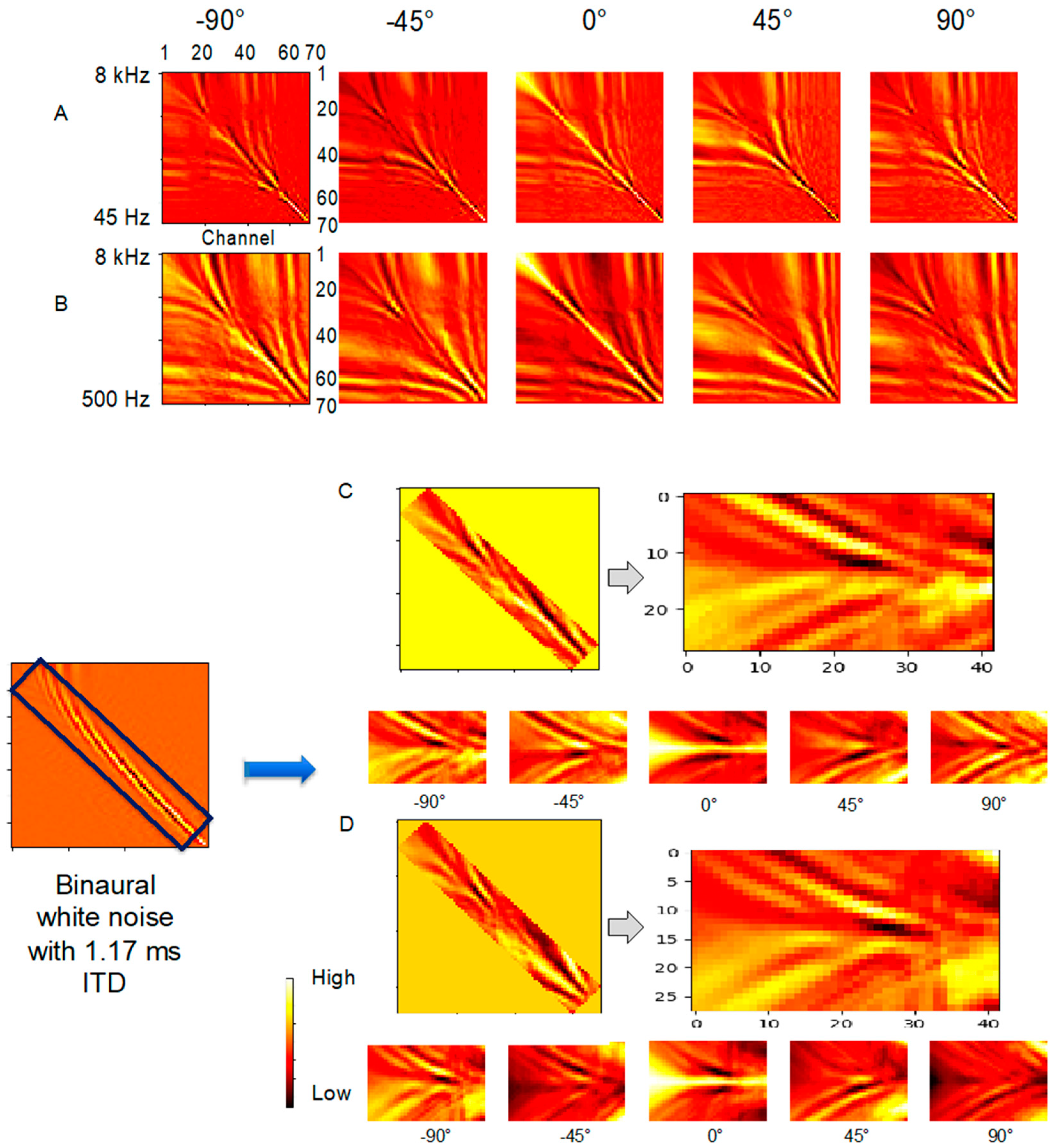
2.2. Modelling the Medial Superior Olive Using Coincidence Detection

In this work, the MSO is modelled by instantaneous correlations between the two CAR-FAC delay lines. At each time t, all the channels from the left CAR-FAC are compared with the right CAR-FAC channels to form a 2-D instantaneous correlogram.

$$Corrlatio{n}_{i,j}\left(i,j,t\right)=z_l\left(i,t\right)\times z_r\left(j,t\right)$$

(2)

$Corrlatio{n}_{i,j}\left(i,j,t\right)$ is the instantaneous correlation at time t between channel i of the left CAR-FAC_L output $z_l\left(i,t\right)$ and channel j of the right CAR-FAC_R output $z_r\left(j,t\right)$.

The instantaneous correlation is approximated by computing the quantised channel outputs:

$${\widehat{Corr}}_{i,j}\left(i,j,t\right)=\{\begin{array}{c}1, if z_l\left(i,t\right)\times z_r\left(j,t\right)>0\\ -1, if z_l\left(i,t\right)\times z_r\left(j,t\right)<0\end{array}$$

(3)

By quantising the instantaneous correlation into a binary range, the resource costs of the hardware implementation are significantly reduced. The FPGA implementation of the instantaneous correlations is described in Reference [36]. The device utilisation of the binaural CAR-FAC and the correlogram implementation on the cyclone V starter kit FPGA board is shown in

Table 1. Device utilisation summary.

	Used	Available	Utilisation
ALM	15,122	29,080	52%
Memory (bits)	1,826,816	4,567,040	40%
DSPs	138	150	92%

.

The quantised instantaneous correlation describes the correlations between two channels. Correlations of the same polarity of the two inputs produce a positive correlation signal, and correlations of the opposite polarity of the two inputs produce a negative anticorrelation signal. Figure 5 illustrates the quantised instantaneous correlation calculation. At time t, channel m of CAR-FAC_L is compared with all the channels of CAR-FAC_R (Only channel m to channel r are shown in Figure 5). The rectangular waves represent the quantised channel output. Within the first m to n channels, the phase shift of CAR-FAC_R with respect to channel m of CAR-FAC_L is smaller than π/2 (in-phase), then the correlations between channel m of CAR-FAC_L and channel m to n of CAR-FAC_R according to equation (2) are positive, denoting correlation. As the wave propagates further in the cascaded structure, the CAR-FAC_R phase shift from channel n to channel p is between π/2 and 3π/2 with respect to channel m of CAR-FAC_L (counter phase). For these channels, the correlations between the two CAR-FACs are negative, denoting anticorrelation. When the wave travels down from channel p to channel r, the CAR-FAC_R phase shift is between 3π/2 and 5π/2 (in-phase), showing correlation again, and so forth. By computing the quantised instantaneous cross-correlations, the ITD between CAR-FAC_L and CAR-FAC_R are actually decided by the interaural phase difference (IPD) of the two cochlear channels. In the Results and Comparisons section, the performance of the non-quantised instantaneous correlation (2) and the quantised instantaneous correlation (3) are compared.

Figure 6 shows the formations of correlograms from different input signals with different ITDs or IPDs. Figure 6A shows an instantaneous correlogram generated from two 200 Hz sine tones with zero delay at time t. Since the two input signals are identical, the two cochlear outputs from each channel have the same phase. This results in the symmetric pattern along the diagonal. The off-diagonal stripes are the results of correlation and anticorrelation of the two cochlear channels at different phases as illustrated in Figure 5. For example, within around the first 55 channels, the phases of CAR-FAC_R channels and channel 1 of CAR-FAC_L are the same, the correlations between channel 1 of CAR-FAC_L and those channels are thus positive (white). As the wave propagates further, the CAR-FAC_R channels and channel 1 of CAR-FAC_L are counter phases, thus the correlations between the two CAR-FACs are negative (black), which is followed by another white and black region. Figure 6B left column shows the correlogram generated by averaging all the instantaneous correlograms during the input signal duration (1 s). At zero delay, the correlogram pattern shows a strong correlation stripe along the diagonal, with symmetric off-diagonal correlation and anticorrelation patterns. Along the series of cochlear channels, there are groups of channels in phase and in counter phase with respect to the other cochlea. Due to the exponentially increased delay of each channel, as an example shown in Figure 4A, the first group has more channels in phase than the second group in counter phase, which again has more channels than the third in-phase group, resulting in curved off-diagonal stripes.

When there is a delay between the two input signals, for example, one input is delayed by a phase of π/2, as shown in Figure 6B middle column, the strongest correlation stripe is shifted off the diagonal towards the cochlea where the signal is delayed, and the off-diagonal bands show an asymmetric structure. The amount of the shift is a measure of the ITD encoded in the correlogram. When the signal is delayed by a phase shift of π, as shown in Figure 6B right column, the input waves are in counter phase and the correlogram pattern is symmetric to the diagonal again. The correlation and anticorrelation are exactly opposite to the zero delay correlogram.

Figure 6C,D shows the correlogram generated from two-tone (800 Hz and 1200 Hz) inputs. Figure 6C shows the CAR-FAC correlogram and Figure 6D shows the CAR only correlogram. We can see strong activations at 800 Hz as well as 1200 Hz in both Figure 6C,D). Furthermore, since the nonlinear CAR-FAC model includes cubic difference tones (CDTs) and quadratic difference tones (QDTs) [37], an additional CDT activation at 2$\times$800 − 1200 = 400 Hz is present in the CAR-FAC correlogram.

To test the correlogram patterns in complex acoustic environments, we use two copies of a Gaussian white noise signal as the input and Figure 6E shows the results. Unlike the sine tones, the white noise is a broadband signal with various frequency components at different times. There is thus no regular in-phase and counter phase waveforms shown along the cochlear channels, except for nearby channels. The correlations of nearby channels correspond to the diagonal with the sideband region in the correlogram. As a result, at zero delay, the white noise correlogram has no significant energy in off-diagonal regions, but a strong correlation band along with black anticorrelation sidebands spaced from the central correlation diagonal. When there is a delay between the two input signals, the strong energy band with correlation and anticorrelation stripes bends to the input that is delayed.

Figure 6F shows the correlogram generated from speech signals. Similar to the noise signal, we can see a strong energy band along the diagonal. In addition to this, off-diagonal stripes are shown in the correlogram. This is because of the formants in the speech cochleogram. The speech travels down along the cochlear channels, presenting strong responses in some channels corresponding to the resonance of the human vocal tract. The regular in-phase and counter phase delays in these channels form correlation and anticorrelation stripes corresponding to the formants.

Figure 6G shows the CAR-FAC correlogram response to a speech signal embedded in Gaussian white noise. The binaural noise with 0, 0.5 ms, and 1 ms delay is added to the speech with zero delay. The middle and lower right regions in the yellow box show the symmetric patterns corresponding to the zero-delay speech, whereas the upper left region in the blue box shows the high-frequency noise component patterns corresponding to the noise with different delays.

The CAR-FAC includes a fast-acting compression via the DOHC model. This produces an adaptively compressed cochlear output. Figure 6H shows the CAR-FAC non-quantised correlogram highlighting the compression effect of the same speech signal as that shown in Figure 6F. The performance of the non-quantised and quantised method is described in the Results and Discussion sections.

2.3. Onset Detection and Onset Correlogram

To decrease interference from echoes and detect the start of a new sound source, a sound onset detection approach is used to generate the correlogram only during the sound onset. The onset detection starts by calculating:

$$∆E\left(t\right)=\log 2\left(\frac{{\sum }_{n=t}^{n=t+step}v{\left(n\right)}^2 }{{\sum }_{n=t-step}^{n=t}v{\left(n\right)}^2}\right)$$

(4)

where $v{\left(n\right)}^2$ is the energy of the sound signal at time n, and step is a time window. $∆E\left(t\right)$ is the logarithmic input energy change at time t. A predefined threshold $∆E\left(t\right)$ is compared with $∆Eth$. If $∆E\left(t\right)\ge ∆Eth$ at time t, the onset time $t$ is detected. When an onset is detected, the onset correlogram is generated by:

$$\widehat{Cor{r}_{onset}}=\frac{1}{∆t\times f_s}\times {\displaystyle \sum }_{t=onset}^{t=onset+∆t}\widehat{Corr\left(t\right)}$$

(5)

where $f_s$ is the sampling frequency and is 44.1 kHz, $onset$ is the detected onset time, ∆t is a short period after the signal onset,$\widehat{Corr\left(t\right)}$ is the 2D instantaneous correlogram at time t, and $\widehat{Cor{r}_{onset}}$ is the averaged quantised instantaneous correlograms during ∆t. The selection of $∆Eth$, ∆t, and the time window are highly depending on the input data and will be discussed in the Experiment and Evaluation section.

The log2 on the right side in (4) is chosen to avoid division on the hardware implementation. The log2 operation can be efficiently implemented on FPGA using a lookup table (LUT) [45,46]. While in human hearing, the onset detection is found in the cochlear nucleus after the cochlea, in this work, the onset detection was implemented before the cochlear. In the hardware implementation, if the onset detection is implemented after the cochlear, a large number of onset detectors are required (one per cochlear channel). It may be helpful in certain conditions where the sound source dominating frequency range is known so that the onset detection from those frequency channels will be more accurate. However, in this work, a single onset detector was sufficient.

2.4. Regression Neural Network

The generated onset correlograms are then analysed using different regression neural networks including linear regression, ELM, and CNN. The linear regression is as a baseline. G. Huang et al. in Reference [47] showed that the ELM can produce good generalisation performance in most cases and can learn thousands of times faster than conventional popular learning algorithms for feedforward neural networks [48,49]. We have implemented the ELM on FPGA [50], so with this set-up, the whole system can be implemented in hardware. Deep CNNs running on GPU platforms represent the current state of the art in image-related problems and natural language processing. CNNs extract important features embedded in the input data and are increasingly computationally efficient. As recent studies have shown the effectiveness of FPGA as a hardware accelerator for the CNNs [51,52,53], the CNN in this system is to be built on FPGA as a real-time and low power consumption system.

The CNN is built using Theano [54], and it consists of two convolutional layers, two pooling layers, one all-to-all connection layer and one output layer, as shown in Figure 1F. For this regression task, the convolutional layer activation function is defined as the rectify function, and the initial weights are set to have the HeUniform distribution [55]. 2 × 2 max-pooling is used in the two pooling layers. The all-to-all connection layer uses a tanh activation function and the initial weights are set as the HeUniform distribution. The output layer has one neuron with a linear activation function. In the training phase, the loss function is defined as the squared-error loss function, and the RMSprop [56] is set as the update rule. The configurations of the CNN are set empirically by testing different settings that are reported to be suitable for a regression task [57,58].

3. Experiment and Evaluation

3.1. Experimental Setup

In the experiment, the binaural data were collected in a reverberant environment, as shown in Figure 7A. In the setup, the sound source incidence angle ranging from −90° to 90° was divided into 13 locations with a 15° step. Two microphones were placed 0.4 m apart from each other on the floor. A speaker was placed 0.96 m away from the centre of the two microphones. The corresponding maximum ITD of this setup is around 1.17 ms (0.4 m/343 m/s). It is within the range of the 70-channel CAR-FAC delay line, 6.5 ms as explained in Figure 4. The setup is thus suitable for investigating the system. We used ten isolated spoken digits (zero to nine) from five speakers in the AusTalk [59,60] database as the sound source, and the spoken digits were played at all 13 locations. A PC connecting to the two microphones recorded the speech to create a binaural signal dataset. Additionally, we augmented the dataset by adding different band-limited noises with different Signal-to-noise ratio (SNRs) (between 15 dBFS and 25 dBFS) and inverting the signal values in the time domain. More details about audio data augmentation can be found in Reference [61]. Through data augmentation, the dataset was enlarged to 11,704 samples.

Figure 7B shows an example of the onset detection in the system. The logarithmic input sound energy change $∆E\left(t\right)$, threshold $∆Eth$, and the time window step are highly signal- and environment-dependent. In this experiment, we found that the threshold $∆Eth$ 3 and step 125 ms in (3) are appropriate for most of the data and thus tend to provide optimal performance. For binaural signals, a separated onset time is detected, and the earliest of the two is used as the onset time. The onset correlogram then is generated 90 ms after the onset, i.e., $∆t$= 90 ms.

3.2. Results and Comparisons

In the CAR-FAC implementation, the total number of channels and the CF range are reconfigurable. Machine hearing models typically use 60 to 100 channels in total [62]. Here, we keep the cochlear channels to 70 and investigate different CF frequency ranges. We limit the upper CF to 8 kHz since the sampling frequency of the original Austalk database is 16 kHz. We first set the lowest CF to 45 Hz, which is close to the lower frequency limit of human hearing. Figure 8A shows generated correlograms at different azimuthal angles. Similar to Figure 6F at zero-delay, it shows strong diagonal correlation and off-diagonal correlation and anticorrelation patterns which correspond to formants of the input speech at 0°. Note that the environmental noise and echoes have resulted in non-symmetric off-diagonal patterns in Figure 6A at zero-delay. When the input speech is played from different azimuthal angles, the generated correlogram shows different patterns that encode different ITD cues. Additionally, the low-frequency channels (bottom-right region) of all the correlograms show blurred off-diagonal patterns in Figure 8A. This is because the input speech does not contain such low-frequency components, so that there is no significant response in these low-frequency channels, and the correlogram in these regions does not encode much information. As we then increase the lowest CF to 500 Hz, to “cut-off” the very low CF channels, the correlograms in these regions show noticeable correlation and anticorrelation stripes in Figure 8B. Since there are more channels above 500 Hz range in the 500 Hz–8 kHz setup, the whole correlogram is clearer than the 45 Hz setup.

The generated 2-D 70 × 70 correlograms ($∆t$= 90 ms) are transformed to have zero mean and fed into different regression neural networks for localisation. The dataset is divided into a training, validation, and testing set. We use the samples from four random speakers as the training data (9324) and the samples from the fifth speaker as the validation (840) and testing data (1540).

Firstly, we use the correlogram generated with the 45 Hz–8 kHz CF range as the input to the neural networks. Inspired by the white noise correlogram in Figure 6D, we select only the diagonal region to reduce the input dimension to the neural network. The diagonal region should encode sufficient ITD cues for the localisation. Furthermore, in this experimental setup, the maximum ITD is 1.17 ms, as explained in the Experiment Setup section. For a binaural white noise signal with a 1.17 ms ITD, the generated correlogram shows a clear pattern in around 14 channels on each side of the diagonal. We, therefore, use 14 channels on each side of the diagonal, which is 42 × 28 diagonal correlogram as the input to the CNN, as shown in Figure 8C,D.

Figure 9 shows the performance of the tests, and the mean and the standard deviation of the results at the 13 locations of the quantised and non-quantised correlograms generated by the CAR and CAR-FAC models. For the ELM, the hidden layer size is set as ten times the input size or 11,760, which is typical for such networks, and the tanh function is used as the nonlinear activation function of the hidden neurons. For the CNN, in the first convolutional layer, the filter number is set to 16, and the convolutional size is set to 19 × 9. In the second convolutional layer, the filter number is set to 32, and the convolutional size is set to 5 × 5. The all-to-all connection layer neuron number is set to 5120. The dropout is set as 0.5 to avoid overfitting. These CNN parameters are set empirically after investigating different configurations and selecting the parameters that result in the best regression performance.

The linear regression shows a large variation of the test localisations around the true locations, the ELM shows improved performance over linear regression, and the CNN shows the closest match to the true locations.

Table 2. Regression results.

		Standard Deviation													Avg. Unsigned Error (°)
		$-90°$	$-75°$	$-60°$	$-45°$	$-30°$	$-15°$	0$°$	$15°$	$30°$	$45°$	$60°$	$75°$	$90°$
CAR-FAC Non Quantised Correlation	Linear	33.65	29.16	18.12	18.30	18.88	17.67	15.66	19.57	19.42	21.28	22.86	27.04	24.50	19.05
	ELM	22.90	17.12	11.64	13.24	12.11	11.81	11.75	11.87	14.50	12.34	12.87	18.92	15.41	13.34
	CNN	6.03	5.35	4.82	4.04	3.19	1.92	0.50	1.26	1.00	0.60	0.45	3.03	4.32	2.87
CAR-FAC Quantised Correlation	Linear	29.00	24.90	23.13	24.64	19.63	17.00	15.81	27.56	17.70	19.59	20.24	27.62	27.10	18.76
	ELM	17.58	15.67	10.87	10.21	11.07	10.99	8.05	10.52	10.68	11.88	14.51	16.40	13.30	13.06
	CNN	11.37	3.03	4.96	3.86	1.04	2.79	2.02	1.92	1.16	1.94	0.61	2.32	5.22	3.11
CAR Non Quantised Correlation	Linear	16.98	16.70	19.18	18.44	19.39	19.61	13.66	17.83	27.81	20.99	17.83	26.00	28.10	16.84
	ELM	11.53	11.23	9.10	11.10	12.15	8.92	9.51	9.9	11.55	9.87	10.92	18.96	11.40	9.35
	CNN	2.76	0.99	4.21	4.80	0.84	2.66	0.38	0.58	0.39	0.16	0.31	1.91	0.33	1.25
CAR Quantised Correlation	Linear	24.05	20.30	23.38	16.50	14.01	17.41	14.06	17.79	17.00	20.61	19.41	21.20	20.86	16.52
	ELM	12.45	10.36	9.92	8.69	8.21	7.53	5.46	7.84	7.04	11.28	8.81	11.80	10.32	8.34
	CNN	6.96	4.04	3.90	2.64	0.17	0.45	0.00	0.26	0.16	0.16	0.22	3.95	1.40	2.74

lists the standard deviation at each location for each case. We can see an increased variance at locations of large azimuthal angles for all the results, especially for the CNN, the largest standard deviation occurs at locations −90° and 90°. As the change of the ITD at large azimuthal angles, e.g., from −90° to −75°, is much smaller than the changes at small azimuthal angles around 0°, the results thus tend to show larger errors in localising the sound source at large azimuthal angles. From the CNN results, we can see the only significant difference is at −90°. The non-quantised correlograms generated by both the CAR and CAR-FAC models show much smaller standard deviations at −90° than the quantised correlograms, as shown in Table 2. This is likely due to the asymmetric noise and echo interference caused by the asymmetric office layout. Additionally, both the non-quantised and quantised correlograms generated by the CAR show slightly smaller averaged unsigned errors than the CAR-FAC, as shown in Table 2.

Secondly, we test correlograms from different CF ranges using the regression CNN. In addition to the diagonal correlogram, a 2 × 2 max-pooling is also used to down-sample the input full correlogram (70 × 70) into size 35 × 35. The RMS errors in the 0–45$°$/45–90$°$ ranges of the quantised and non-quantised correlograms generated by both the CAR and CAR-FAC models are listed in

Table 3. Regression results.

CF Range/Damping		Diagonal Correlogram	$2\times 2$ Max-Pooling Correlogram
		RMS Error (°) 0–45°/45–90°	RMS Error (°) 0–45°/45–90°
CAR-FAC Non-quantised Correlation	45 Hz–8 kHz	2.78/5.60	4.88/9.15
	500 Hz–8 kHz	4.48/6.86	3.02/6.22
CAR-FAC Quantised Correlation	45 Hz–8 kHz	2.92/7.12	3.51/7.62
	500 Hz–8 kHz	2.21/6.88	2.44/6.62
CAR Non-quantised Correlation	45 Hz–8 kHz	2.55/3.28	4.39/5.41
	500 Hz–8 kHz	1.92/3.79	2.72/4.83
CAR Quantised Correlation	45 Hz–8 kHz	1.82/5.97	2.82/4.26
	500 Hz–8 kHz	3.18/3.70	3.46/4.21

. The diagonal approach tends to provide smaller 0–45$°$/45–90$°$ RMS errors for the 45 Hz to 8 kHz frequency range when the non-quantised correlograms generated by both the CAR and CAR-FAC models are used. Both the max-pooling and diagonal approaches show smaller 45−90$°$ RMS errors for the 500 Hz to 8 kHz frequency range than the 45 Hz to 8 kHz range when the quantised correlograms generated by either the CAR or CAR-FAC models are used. Although the 500 Hz to 8 kHz CF range correlograms show clearer patterns in Figure 8A,B than the 40 Hz to 8kHz range, the results from Table 3 did not show significant differences in the RMS errors between them. The CNN is able to extract essential features from both of the correlograms for localising a sound source.

Figure 10 shows the CNN results of the quantised correlograms generated by the CAR model. With proper settings of cochlear CF ranges and pooling approaches, the quantised correlograms show reduced standard deviations at large azimuthal angles and excellent matches to the true sound source locations. For example, the 500 Hz to 8 kHz frequency range shows smaller standard deviation than the 40 Hz to 8 kHz frequency range at −90° when the diagonal correlogram is used, which indicates our simplest hardware implementation is sufficient for this task.

Table 4. Comparisons of sound localisation systems.

System	Mic	Cues	Stimulus	Accuracy	Approach
				0–45°/45–90°
[17]	2	ITD	Periodic clicks (475 Hz)	N/A	Two silicon cochlear models and the Jeffress model on chip
[21]	2	ITD	Sine tones, white noises, and vowels	N/A	Instantaneous cross correlation with two silicon cochlear models on chip
[23]	2	ITD	N/A	N/A	Propose FPGA implementation of the cochlear model, LIF neuron model and WTA network
[20]	4	IPD, IED, IID, Spectral cues	Impulse	5° RMS error (azimuth and elevation)	Three-chip system; One for onset detection, one for BPF bank and IED/IID cue extraction, and one for cross-correlation, IPD
[22]	2	ITD	(50–300 Hz) sounds	3°/12° RMS error	Two silicon cochleae, zero-crossing
[63]	4	ITD	<300 Hz	3°/8° RMS error	Digital delay line on chip
[26]	2	ITD	FM Noise, Alarm Bell	FM Noise * RMS error 9.27°/12.48° Alarm Bell * 42.7°/54.76°	Delay line and CONP on FPGA
[64]	2	IID	Pure tones	1.09°/0.70° RMS error	Event-based cochleae, IID, “head” movement
[27]	2	ITD	Noise, Sine tones	2.7°/5.5° RMS error	Two silicon cochleae (AER-EAR)
This work	2	ITD(IPD)	Spoken digits in office	2.82°/4.26° RMS error Or 1.32°/2.93° unsigned average error	CAR pair CNN
Human [62]	2 ears	Binaural processing	Broadband sound sources	4.03°/7.03° azimuth ** unsigned average error	Brief (150 ms) sound presented in front of 6 subjects in a free field

* The RMS error is converted from the recognition rates in Reference [26]. ** The unsigned average error is converted from TABLE I in References [65,66] at 5° elevation.

shows comparisons of the proposed system with other biologically inspired sound localisation systems [26,63,64]. Human sound localisation performance reported in Reference [65] is also included in the table.

4. Discussion

In this paper, we have presented a biologically inspired binaural sound localisation system for reverberant environments. It uses a binaural CAR-FAC system to pre-process the binaural signal, 2-D correlograms to encode the interaural time difference (ITD) cues, and a regression network to learn the azimuthal angle of the sound source. We found that in this application, the nonlinearity of the FAC did not improve performance. The linear CAR model showed smaller averaged unsigned errors.

This work provides a baseline of binaural sound localisation using the CAR and CAR-FAC in a reverberant environment. As such, most of the parameters of the CAR and CAR-FAC, the onset detection, and the CNN were empirically chosen for the best performance under the investigated environments. For example, the CAR-FAC are configurated to a 70-channel ‘delay line’ with a propagation delay of 6.5 ms, and more channels can extend the delay for a higher ITD detecting range. The delay also changes when you choose different CF ranges. The onset detection is used to decrease interference from echoes and detect the start of a new sound source.

The use of quantised instantaneous correlations makes the system easily implementable on hardware without much performance loss, as shown in Figure 9. A possible further improvement of correlogram generation for noisier environments is to set a threshold in the quantisation in (3) to decrease noise sensitivity. The ELM results show the quantised correlograms from both the CAR and CAR-FAC are able to provide a suitable basis with which to perform sound localisation tasks. The use of the CNN significantly improves the system accuracy. The CNN is able to extract essential features from the noisy correlogram for localising a sound source. The correlogram is able to encode the formants of speech signals, so that the system can be extended to other auditory tasks such as speech recognition. From Figure 6G, we have seen that with the CAR-FAC pre-processing, different frequency components from different sound source locations can form different patterns in different correlogram regions. Another potential application of this system can thus be sound source segregation.

5. Conclusions

We present a biologically inspired sound localisation system for reverberant environments and investigate its performance using speech data recorded in our office. We investigated the CAR-FAC configurations, correlogram generation approaches, and regression networks of the system. We found quantised 2-D correlograms generated from a binaural CAR system and analysed with a CNN have shown small RMS localisation errors. Therefore, in such high SNR conditions, a linear CAR with a quantised correlogram generation can provide sufficient accuracy with less hardware resource constraints.

References

1. Grothe, B.; Neuweiler, G. The function of the medial superior olive in small mammals: Temporal receptive fields in auditory analysis. J. Comp. Physiol. A Sens. Neural Behav. Physiol. 2000, 186, 413–423. [Google Scholar] [CrossRef] [PubMed]
2. Yin, T.C.T. Neural mechanisms of encoding Binaural localization cues in the auditory brainstem. In Integrative Functions in the Mammalian Auditory Pathway; Springer: Berlin, Germany, 2002; Volume 15, pp. 99–159. [Google Scholar]
3. Park, T.J.; Klug, A.; Holinstat, M.; Grothe, B. Interaural level difference processing in the lateral superior olive and the inferior colliculus. J. Neurophysiol. 2004, 92. [Google Scholar] [CrossRef] [Green Version]
4. Rayleigh, L. On our perception of sound direction. Philos. Mag. 1907, 13, 214–232. [Google Scholar] [CrossRef] [Green Version]
5. Zwislocki, J.; Feldman, R.S. Just noticeable differences in dichotic phase. J. Acoust. Soc. Am. 1956, 28, 860–864. [Google Scholar] [CrossRef]
6. Casseday, J.H.; Neff, W.D. Localization of pure tones. J. Acoust. Soc. Am. 1973, 54, 365–372. [Google Scholar] [CrossRef]
7. Henning, G.B. Detectability of interaural delay in high-frequency complex waveforms. J. Acoust. Soc. Am. 1974, 55, 84–90. [Google Scholar] [CrossRef]
8. Batra, R.; Kuwada, S.; Stanford, T.R. Temporal coding of envelopes and their interaural delays in the inferior colliculus of the unanesthetized rabbit. J. Neurophysiol. 1989, 61, 257–268. [Google Scholar] [CrossRef] [PubMed]
9. Joris, P.X. Envelope coding in the lateral superior olive. II. Characteristic delays and comparison with responses in the medial superior olive. J. Neurophysiol. 1996, 76, 2137–2156. [Google Scholar] [CrossRef]
10. Grothe, B.; Pecka, M.; McAlpine, D. Mechanisms of Sound localization in mammals. Physiol. Rev. 2010, 90, 983–1012. [Google Scholar] [CrossRef] [PubMed] [Green Version]
11. Yin, T.C.T.; Kuwada, S. Binaural localization cues. In The Oxford Handbook of Auditory Science: The Auditory Brain; Oxford University Press: Oxford, UK, 2012. [Google Scholar]
12. Lyon, R.F. A computational model of binaural localization and separation. In Proceedings of the ICASSP, IEEE International Conference on Acoustics, Speech and Signal Processing, Boston, MA, USA, 14–16 April 1983. [Google Scholar]
13. Shamma, S.A.; Shen, N.; Gopalaswamy, P. Stereausis: Binaural processing without neural delays. J. Acoust. Soc. Am. 1989, 86. [Google Scholar] [CrossRef]
14. Jeffress, L.A. A place theory of sound localization. J. Comp. Physiol. 1948, 41, 35–39. [Google Scholar] [CrossRef]
15. Heckmann, M.; Rodemann, T.; Joublin, F.; Goerick, C.; Schölling, B. Auditory inspired binaural robust sound source localization in echoic and noisy environments. In Proceedings of the IEEE International Conference on Intelligent Robots and Systems, Beijing, China, 9–15 October 2006. [Google Scholar]
16. Joris, P.X.; van Der Heijden, M. Early Binaural hearing: The Comparison of temporal differences at the two ears. Annu. Rev. Neurosci. 2019, 42, 433–457. [Google Scholar] [CrossRef] [PubMed]
17. Lazzaro, J.; Mead, C. A silicon model of auditory localization. Neural Comput. 1989, 1, 47–57. [Google Scholar] [CrossRef] [Green Version]
18. Ashida, G.; Carr, C.E. Sound localization: Jeffress and beyond. Curr. Opin. Neurobiol. 2011, 21, 745–751. [Google Scholar] [CrossRef] [Green Version]
19. Bhadkamkar, N.; Fowler, B. A sound localization system based on biological analogy. In Proceedings of the 1993 IEEE International Conference on Neural Networks, San Francisco, CA, USA, 28 March–1 April 1993; pp. 1902–1907. [Google Scholar]
20. Grech, I.; Micallef, J.; Vladimirova, T. Analog CMOS chipset for a 2-D sound localization system. Analog. Integr. Circuits Signal. Process. 2004, 41, 167–184. [Google Scholar] [CrossRef]
21. Mead, C.; Arreguit, X.; Lazzaro, J. Analog VLSI model of binaural hearing. IEEE Trans. Neural Netw. 1991, 2, 230–236. [Google Scholar] [CrossRef] [PubMed] [Green Version]
22. van Schaik, A.; Shamma, S. A neuromorphic sound localizer for a smart MEMS system. Analog Integr. Circuits Signal. Process 2004, 39, 267–273. [Google Scholar] [CrossRef]
23. Ponca, M.; Schauer, C. FPGA implementation of a spike-based sound localization system. In Artificial Neural Networks and Genetic Algorithms; Springer: Berlin/Heidelberg, Germany, 2001. [Google Scholar]
24. Finger, H.; Liu, S.C. Estimating the location of a sound source with a spike-timing localization algorithm. In Proceedings of the IEEE International Symposium on Circuits and Systems, Rio de Janeiro, Brazil, 15–18 May 2011. [Google Scholar]
25. Iwasa, K.; Kugler, M.; Kuroyanagi, S.; Iwata, A. A sound localization and recognition system using pulsed neural networks on FPGA. In Proceedings of the International Joint Conference on Neural Networks (IJCNN), Orlando, FL, USA, 12–17 August 2007; pp. 902–907. [Google Scholar]
26. Kugler, M.; Iwasa, K.; Benso, V.A.; Kuroyanagi, S.; Iwata, A. A complete hardware implementation of an integrated sound localization and classification system based on spiking neural networks. Neural Inf. Process. 2008, 4985, 577–587. [Google Scholar]
27. Chan, V.Y.S.; Jin, C.T.; van Schaik, A. Adaptive sound localization with a silicon cochlea pair. Front. Neurosci. 2010, 4, 1–31. [Google Scholar] [CrossRef] [PubMed] [Green Version]
28. Schauer, C.; Zahn, T.; Paschke, P.; Gross, H.M. Binaural sound localization in an artificial neural network. In Proceedings of the ICASSP, IEEE International Conference on Acoustics, Speech and Signal Processing, Istanbul, Turkey, 5–9 June 2000. [Google Scholar]
29. Youssef, K.; Argentieri, S.; Zarader, J.L. A learning-based approach to robust binaural sound localization. In Proceedings of the IEEE International Conference on Intelligent Robots and Systems, Tokyo, Japan, 3–7 November 2013. [Google Scholar]
30. Ma, N.; May, T.; Brown, G.J. Exploiting deep neural networks and head movements for robust binaural localization of multiple sources in reverberant environments. IEEE ACM Trans. Audio Speech Lang. Process. 2017, 25, 2444–2453. [Google Scholar] [CrossRef] [Green Version]
31. Wang, J.; Wang, J.; Qian, K.; Xie, X.; Kuang, J. Binaural sound localization based on deep neural network and affinity propagation clustering in mismatched HRTF condition. Eurasip J. Audio Speech Music Process. 2020. [Google Scholar] [CrossRef] [Green Version]
32. Jiang, S.; Wu, L.; Yuan, P.; Sun, Y.; Liu, H. Deep and CNN fusion method for binaural sound source localisation. J. Eng. 2020, 2020, 511–516. [Google Scholar] [CrossRef]
33. Xu, Y.; Afshar, S.; Singh, R.K.; Hamilton, T.J.; Wang, R.; van Schaik, A. A machine hearing system for binaural sound localization based on instantaneous correlation. In Proceedings of the 2018 IEEE International Symposium on Circuits and Systems (ISCAS), Florence, Italy, 27–30 May 2018. [Google Scholar]
34. Wallach, H.; Newman, E.B.; Rosenzweig, M.R. The precedence effect in sound localization. Am. J. Psychol. 1949, 62, 315–336. [Google Scholar] [CrossRef] [PubMed]
35. Wühle, T.; Merchel, S.; Altinsoy, M.E. The precedence effect in scenarios with projected sound. AES J. Audio Eng. Soc. 2019, 67, 92–100. [Google Scholar]
36. Xu, Y.; Afshar, S.; Singh, R.K.; Wang, R.; van Schaik, A.; Hamilton, T.J. A binaural sound localization system using deep convolutional neural networks. In Proceedings of the IEEE International Symposium on Circuits and Systems, Sapporo, Japan, 26–29 May 2019. [Google Scholar]
37. Lyon, R.F. Human and Machine Hearing—Extracting Meaning from Sound; Cambridge University Press: Cambridge, UK, 2017. [Google Scholar]
38. Xu, Y.; Singh, R.K.; Thakur, C.S.; Wang, R.; van Schaik, A. CAR-FAC Model of the cochlea on the FPGA. In Proceedings of the BioMedical Circuits and Systems Conference (BIOCAS), Shanghai, China, 17–19 October 2016; pp. 1–4. [Google Scholar]
39. Xu, Y.; Thakur, C.S.; Singh, R.K.; Hamilton, T.J.; Wang, R.M.; van Schaik, A. A FPGA implementation of the CAR-FAC cochlear model. Front. Neurosci. 2018, 12, 1–14. [Google Scholar] [CrossRef]
40. Greenwood, D.D. A cochlear frequency-position function for several species—29 years later. J. Acoust. Soc. Am. 1990, 87, 2592–2605. [Google Scholar] [CrossRef]
41. Singh, R.K.; Xu, Y.; Wang, R.; Hamilton, T.J.; van Schaik, A.; Denham, S.L. CAR-lite: A Multi-rate cochlear model on FPGA for Spike-based sound encoding. IEEE Trans. Circuits Syst. I Regul. Pap. 2018, 66, 1805–1817. [Google Scholar] [CrossRef]
42. Singh, R.K.; Xu, Y.; Wang, R.; Hamilton, T.J.; van Schaik, A.; Denham, S.L. CAR-lite: A Multi-rate cochlea model on FPGA. In Proceedings of the IEEE International Symposium on Circuits and Systems, Florence, Italy, 27–30 May 2018. [Google Scholar]
43. Katsiamis, A.G.; Drakakis, E.M.; Lyon, R.F. Practical gammatone-like filters for auditory processing. Eurasip J. Audio Speech Music Process. 2007. [Google Scholar] [CrossRef] [Green Version]
44. Chi, T.; Ru, P.; Shamma, S.A. Multiresolution spectrotemporal analysis of complex sounds. J. Acoust. Soc. Am. 2005, 118. [Google Scholar] [CrossRef] [Green Version]
45. Seidner, D. Efficient implementation of log10 lookup table in FPGA. In Proceedings of the IEEE International Conference on Microwaves, Communications, Antennas and Electronic Systems, Tel-Aviv, Israel, 13–14 May 2008; pp. 1–9. [Google Scholar]
46. Bangqiang, L.; Ling, H.; Xiao, Y. Base-N logarithm implementation on FPGA for the data with random decimal point positions. In Proceedings of the IEEE 9th International Colloquium on Signal Processing and Its Applications (CSPA), Kuala Lumpur, Malaysia, 8–10 March 2013. [Google Scholar]
47. Huang, G.; Zhu, Q.-Y.; Siew, C.-K. Extreme learning machine: Theory and applications. Neurocomputing 2006, 70, 489–501. [Google Scholar] [CrossRef]
48. McDonnell, M.D.; Tissera, M.D.; Vladusich, T.; van Schaik, A.; Tapson, J. Fast, simple and accurate handwritten digit classification by training shallow neural network classifiers with the ‘extreme learning machine’ algorithm. PLoS ONE 2015, 10, 1–18. [Google Scholar] [CrossRef] [PubMed] [Green Version]
49. van Schaik, A.; Tapson, J. Online and adaptive pseudoinverse solutions for ELM weights. Neurocomputing 2015, 149, 233–238. [Google Scholar] [CrossRef] [Green Version]
50. Wang, R.; Cohen, G.; Thakur, C.S.; Tapson, J.; van Schaik, A. An SRAM-based implementation of a convolutional neural network. In Proceedings of the IEEE Biomedical Circuits and Systems Conference, Shanghai, China, 17–19 October 2016; pp. 1–4. [Google Scholar]
51. Kala, S.; Jose, B.R.; Mathew, J.; Nalesh, S. High-performance CNN accelerator on FPGA using unified winograd-GEMM architecture. IEEE Trans. Very Large Scale Integr. Syst. 2019, 27, 2816–2828. [Google Scholar] [CrossRef]
52. Nguyen, D.T.; Nguyen, T.N.; Kim, H.; Lee, H.J. A high-throughput and power-efficient fpga implementation of yolo CNN for object detection. IEEE Trans. Very Large Scale Integr. Syst. 2019, 27, 1861–1873. [Google Scholar] [CrossRef]
53. Lian, X.; Liu, Z.; Song, Z.; Dai, J.; Zhou, W.; Ji, X. High-performance FPGA-based CNN accelerator with block-floating-point arithmetic. IEEE Trans. Very Large Scale Integr. Syst. 2019, 27, 1874–1885. [Google Scholar] [CrossRef]
54. Al-Rfou, R. Theano: A Python Framework for Fast Computation of Mathematical Expressions; Cornell University: Ithaca, NY, USA, 2016. [Google Scholar]
55. He, K.; Zhang, X.; Ren, S.; Sun, J. Delving deep into rectifiers: Surpassing human-level performance on imagenet classification. In Proceedings of the IEEE International Conference on Computer Vision, Santiago, Chile, 7–13 December 2015. [Google Scholar]
56. Ruder, S. An Overview of Gradient Descent Optimization Algorithms; Cornell University: Ithaca, NY, USA, 2016; pp. 1–14. [Google Scholar]
57. Theano Development Team. Theano: A Python Framework for Fast Computation of Mathematical Expressions; Cornell University: Ithaca, NY, USA, 2016. [Google Scholar]
58. Zhou, J.; Hong, X.; Su, F.; Zhao, G. Recurrent convolutional neural network regression for continuous pain intensity estimation in video. In Proceedings of the IEEE Computer Society Conference on Computer Vision and Pattern Recognition Workshops, Las Vegas, NV, USA, 26 Jun–1 July 2016. [Google Scholar]
59. Burnham, D.; Ambikairajah, E.; Arciuli, J.; Bennamoun, M.; Best, C.T.; Bird, S.; Butcher, A.R.; Cassidy, S.; Chetty, G.; Cox, F.M.; et al. A blueprint for a comprehensive Australian English auditory-visual speech corpus. In Selected Proceedings of the 2008 HCSNet Workshop on Designing the Australian National Corpus; Cascadilla Proceedings Project: Somerville, MA, USA; pp. 96–107.
60. Burnham, D.; Estival, D.; Fazio, S.; Viethen, J.; Cox, F.; Dale, R.; Cassidy, S.; Epps, J.; Togneri, R.; Wagner, M. Building an audio-visual corpus of Australian English: Large corpus collection with an economical portable and replicable black box. In Proceedings of the Annual Conference of the International Speech Communication Association (INTERSPEECH), Florence, Italy, 27–31 August 2011; pp. 841–844. [Google Scholar]
61. Ko, T.; Peddinti, V.; Povey, D.; Khudanpur, S. Audio augmentation for speech recognition. In Proceedings of the Annual Conference of the International Speech Communication Association (INTERSPEECH), Dresden, Germany, 6–10 September 2015. [Google Scholar]
62. Lyon, R.F. Cascades of two-pole-two-zero asymmetric resonators are good models of peripheral auditory function. J. Acoust. Soc. Am. 2011, 130, 3893–3904. [Google Scholar] [CrossRef] [PubMed] [Green Version]
63. Julian, P.; Andreou, A.G.; Goldberg, D.H. A low-power correlation-derivative CMOS VLSI circuit for bearing estimation. IEEE Trans. Very Large Scale Integr. Syst. 2006, 14, 207–212. [Google Scholar] [CrossRef]
64. Escudero, E.C.; Peña, F.P.; Vicente, R.P.; Jimenez-Fernandez, A.; Moreno, G.J.; Morgado-Estevez, A. Real-time neuro-inspired sound source localization and tracking architecture applied to a robotic platform. Neurocomputing 2018, 283, 129–139. [Google Scholar] [CrossRef]
65. Middlebrooks, J.C.; Green, D.M. Sound localization by human listeners. Annu. Rev. Psychol. 1991, 42, 135–159. [Google Scholar] [CrossRef]
66. Carlile, S.; Leong, P.; Hyams, S. The nature and distribution of errors in sound localization by human listeners. Hear. Res. 1997, 114, 179–196. [Google Scholar] [CrossRef]
Figure 1. Architecture of the binaural sound localisation system. (A) The Cascade of Asymmetric Resonators with Fast-Acting Compression (CAR-FAC) model, H1 to HN are the transfer functions of the CAR part, the centre frequencies (CFs) of the resonators decrease from H1 to HN. The digital outer hair cell (DOHC), the digital inner hair cell (DIHC), and the automatic gain control (AGC) comprise the FAC part. The DIHC output is connected to the lateral inhibition (LI) function. (B) The LI unit; (C) The instantaneous correlogram: the circle marked with a cross is an instantaneous correlation unit, and the output from all the units forms a 2-D correlogram. (D) The onset detection function; (E) The onset correlogram; a short period after the onset detection, t 1 to t n , includes n instantaneous correlograms. The n instantaneous correlograms are averaged to form the onset correlogram. (F) The regression convolutional neural network (CNN); the onset correlogram is used to train the CNN to learn the azimuthal angle of the sound source. The details of the CNN will be described later in the Experiments and Evaluation section. In this system, the binaural CAR FAC and the onset correlogram have been implemented on Field Programmable Gate Array (FPGA), and the onset detection and the CNN were implemented on a PC, but can also be ported to FPGA.
Applsci 11 01519 g001
Figure 2. The binaural CAR-FAC system architecture. The system consists of an audio codec, a controller, a synchronisation circuit, an external Double Data Rate Synchronous Dynamic Random Access Memory (DDR) and two ‘ears’. Each ear includes a CAR FAC module. The system provides two ways for sound input. One way is through the SSM2603 audio codec on the FPGA board, and a second provides recorded audio file input from the PC host through a USB 3.0 interface. There are two clock domains in the system: a system clock domain (250 MHz) and a synchronisation clock domain (100 MHz). The system clock domain includes the controller, the two CAR-FACs, and the Correlogram module. The synchronisation clock domain is unique to the synchronisation unit. The external memory is a 1 GB DDR3 SDRAM on the FPGA board: it stores the CAR-FAC output or the correlogram via a selector. The USB interface communicates between the FPGA board and the PC, and transmits the system’s initial parameters, and, if required, the input audio file from the PC to the FPGA board. The controller state machine determines the cochlear channel to be processed at any particular time and controls the CAR-FAC coefficients and data for that channel. The BM_start signal controls the start of the system through the controller, and it is triggered by the “Audio_in ready” signal. The ohc_sel is a selector switch for the CAR/CAR-FAC function. The agc_sel is a switch for the AGC loop function. The CAR state machine calculates the CAR transfer function and controls the DOHC and DIHC_AGC start in the system. The DOHC state machine calculates OHC function and feeds back an updated r to the CAR. The DIHC-AGC calculates the IHC function, as well as the AGC_loop function. The AGC output b feeds back to the DOHC module. The details of the module are presented in References [38,39]. The DIHC-LI outputs of the two ‘ears’ are used to generate correlograms in the correlogram module, which is presented in Reference [36]. The FPGA board is hosted by a PC through the USB interface.
Applsci 11 01519 g002
Figure 3. CAR-FAC basilar membrane (BM) response to (A) a 500 Hz sine tone at six channels along the travelling wave structure and (B) 70-channel response at an instant in time. (C) a click (a short and sharp sound) at seven channels along the travelling wave structure and (D) 70-channel response at 3 different times. (E) a 200 Hz and 800 Hz tone at seven channels along the travelling wave structure and (F) 70-channel response at an instant in time.
Applsci 11 01519 g003
Figure 4. (A) Delay of CAR-FAC channels against centre frequency (CF) to a speech and delay of each CAR-FAC channel; (B) The CAR-FAC IHC (blue) and the lateral inhibition (red) response to a 500 Hz sine wave on its CF channel (CF corresponds to 500 Hz).
Applsci 11 01519 g004
Figure 5. Quantised instantaneous cross-correlation calculation schematic diagram: The phase shift of the CAR-FAC_R (channel m to channel r) with respect to channel m of CAR-FAC_L at time t. The magenta circles mark the phases of different channels at time t.
Applsci 11 01519 g005
Figure 6. CAR-FAC quantised instantaneous correlogram (3) generated in response to (A) two 200 Hz sine tone at time t at zero delay; and averaged correlogram generated over the input duration in response to (B) two 200 Hz sine tone at zero, π/2, and π radians delay; (C) 800 Hz and 1200 Hz sine tones at 0, 0.5 ms, and 1 ms delays; (D) 800 Hz and 1200 Hz sine tones at 0, 0.5 ms, and 1 ms delays generated using the CAR only; (E) two white noise signals at 0, 0.5 ms, and 1 ms delays; (F) two speech signals, spoken digit “eight”, at 0, 0.5 ms, and 1 ms delays; and (G) two noisy speech signals at 0, 0.5 ms, and 1 ms noise delays. Note the speech is zero-delay in this example; (H) CAR-FAC non-quantised correlogram (2) generated in response to the same speech as in (F).
Applsci 11 01519 g006
Figure 7. (A) Experiment setup in a reverberant environment (an office); (B) Onset detection; the log-energy change E of the spoken digit ‘six’ (blue) is shown in red and green, and the circles mark the detected onset time for each input of the binaural signal. The first onset time t is selected to be the onset time. Adapted from Reference [33].
Applsci 11 01519 g007
Figure 8. Onset correlogram generated from speech “eight”. (A) CAR-FAC filter CF frequency range is from 45 Hz to 8 kHz; (B) CAR-FAC filter CF frequency range is from 500 Hz to 8 kHz. Five azimuthal angles (−90°, −45°, 0°, 75°, and 90°) are shown here, and correlogram generated from a binaural white noise with 1.17 ms ITD (Bottom left) and (Bottom right) used as the input of the CNN. 14 channels on each side of the diagonal of the correlogram are selected, and the top left and bottom right of the correlogram are discarded to form a rectangular input to the CNN. (C) Diagonal correlogram of speech “eight” and (D) “zero” at location −90°, −45°, 0°, 45°, and 90°.
Applsci 11 01519 g008
Figure 9. Comparisons of the linear regression (top), ELM regression (middle), and CNN regression (bottom) on the experimental data. The true location is shown in blue square, and the testing data result is shown in red round.
Applsci 11 01519 g009
Figure 10. CNN results with different CAR configurations and different quantised correlogram inputs.
Applsci 11 01519 g010