Flexible Job Shop Scheduling Problem with Sequence Dependent Setup Time and Job Splitting: Hospital Catering Case Study

Abstract

This paper aims to study a real case of an optimization problem derived from a hospital supply chain. The present work focuses on developing operational decision support models and algorithms for production process scheduling in hospital catering. The addressed production system is considered as a flexible job shop system. The objective is to minimize the total flow time. A novel mathematical model and two metaheuristics for the production scheduling of multi-product and multi-stage food processes are developed. These methods have proven their effectiveness for the scheduling of operations of the food production processes and allowed significant improvements in the performance of the studied production system.

1. Introduction

Nowadays, hospital logistics has become an essential component of healthcare institutions. It allows the synchronization of all the flows inside a hospital to ensure the efficiency of the healthcare system. For many years, the management was commonly focused on improving the quality of medical care, while less attention was usually devoted to operation management. In recent years, the need for containing the costs while increasing the competitiveness along with the new national health service policies for hospital financing forced hospitals to necessarily improve their operational efficiency. It is in this context that the efficient use of resources and the research on optimal service stimulate logistical thinking in hospitals. The difficulties of optimizing flows have led managers to discover new avenues for rationalizing expenses and seeking refined solutions to these difficulties. In this context, optimized logistics solutions allow hospitals to improve inventory management, limit waste, and provide better inventory tracking and traceability of service products. On the other hand, the supply chain is a major source of costs, and its reorganization would make it possible to achieve crucial savings on all hospital expenses.

A hospital’s logistics is part of its global performance, where the activities are organized and structured with the aim of patients’ satisfaction in terms of quality, quantity, delay, safety, and low cost. The main purpose of this logistics is to control and optimize physical flows from suppliers to patients at the best cost that respects technical, economic, and regulatory conditions for optimal dispensing to patients. Hospital logistics is a complex process characterized by a diversity of needs, users, products, and distribution channels. The coordination of these activities requires logistical expertise that few institutions will be able to develop on their own. This has led researchers to focus for some years on the management and optimization of the supply chain in hospitals. In this context and in order to improve the working conditions of the employees and their well-being, the hospital center of Troyes implements means to improve its daily efficiency. The hospital is carrying out a revision of its supply chain, which must notably consider the management of food flows within the hospital. In the present work, we focused particularly on the scheduling of the food manufacturing process in hospital catering, which is considered as a flexible job shop scheduling problem with a sequence-dependent setup time and job splitting by integrating specific industrial constraints.

The remainder of this paper is organized as follows: Section 2 presents the state of the art regarding the problem of food production process scheduling. The problem statement is defined in Section 3. In Section 4, the mathematical model developed for the studied problem is presented. Section 5 and Section 6 present the genetic and the iterated local search algorithms specifically developed for the problem, the different elements of these metaheuristics, and the computational results. Finally, in the last section, an application to a real industrial case and the results obtained are presented.

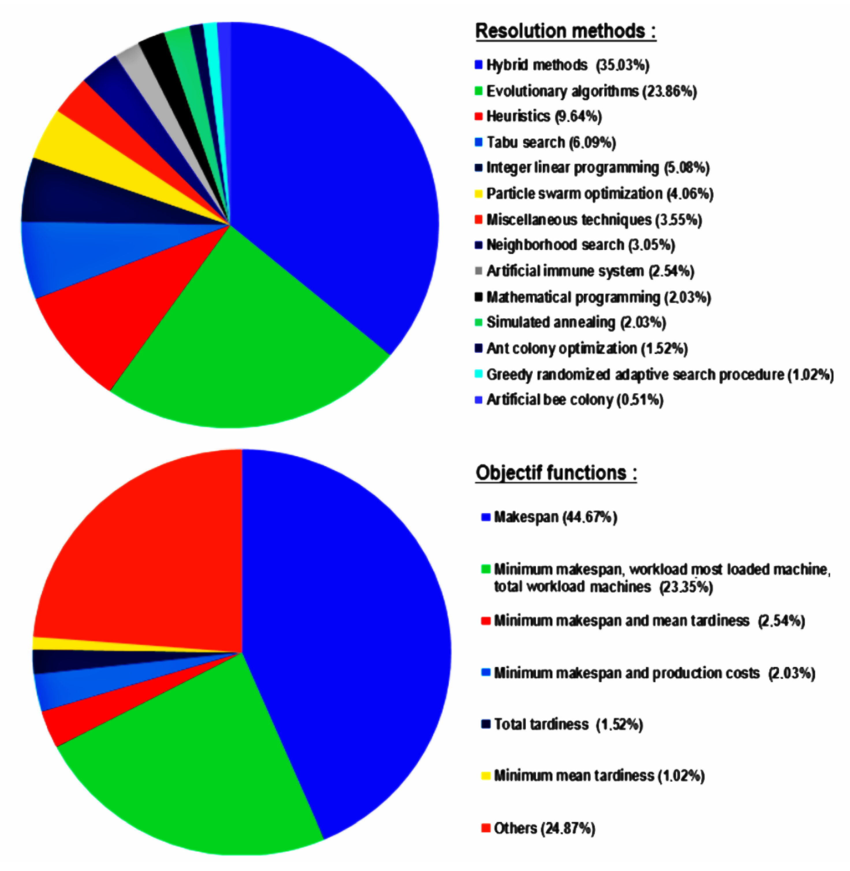
2. Literature Review

The production scheduling problem in food industries belongs to a famous class of problems referred to as scheduling with sequence-dependent setups, which are well known to be NP-hard (Sun et al. [1]). In recent years, there has been great interest in the development of intelligent solutions for this problem in various fields of application. The promising results of scheduling methods, such as reduction of production costs, increased throughput and smoother operation of the production equipment, and improvement of working conditions and the well-being of employees, have stimulated considerable research efforts. The existing works in the literature are classified according to the number of products (single products or multiple products), the type of production system, and the expiration dates of products, which may be known or unknown.

Regarding works dealing with a single product, Entrup et al. [2] proposed three different mixed-integer linear programming for scheduling problems in the packing stage of stirred yogurt production in the fresh food industry. They accounted for shelf life issues and fermentation capacity limitations. Doganis and Sarimveis [3] proposed a model that aims to obtain the optimal production scheduling in a single yogurt production line. The model takes into account all the standard constraints encountered in production scheduling (material balances, inventory limitations, machinery capacity). It also considers special features that characterize yogurt production and that are limitations in production sequencing, mainly due to different fat contents and flavors of various products, as well as sequence-dependent setup times and costs. However, the model is limited to a single production line. In another study, Doganis and Sarimveis [4] presented a methodology for optimum scheduling of yogurt packaging lines that consist of multiple parallel machines. The methodology incorporates features that allow one to tackle industry-specific problems, such as multiple intermediate due dates, job mixing and splitting, product-specific machine speed, minimum and maximum lot size, and sequence-dependent changeover times and costs. However, the proposed mathematical model does not incorporate multi-stage production decisions and ignores some industry-specific characteristics, such as shelf life. Stefansdottir et al. [5] developed a generic optimization model for lot sizing and scheduling in the typical processing industry setting of flow shops. Sargut and Isık [6] presented a mathematical model for a dynamic economic lot sizing problem with a single machine for a single perishable item under production capacities. They also gave a dynamic programming-based heuristic for the solution of the overall problem.

Many studies have been carried out in the literature on the production scheduling of multi-product food processing industries. Akkerman and van Donk [7] developed a methodology for the analysis of the scheduling problems in food processing. This helps one to understand, describe, and structure scheduling problems in food processing and to evaluate the organizational structures and information flows related to scheduling. Smith, Daniels, and Larry [8] developed a general lot-sizing model for processing industries and applied their method to a representative situation of a food processing facility. Kopanos et al. [9] offered an efficient mathematical framework for detailed production scheduling in the food processing industry. Wauters et al. [10] introduced an integrated approach for production scheduling and demonstrated its applicability to the food processing industry. In this work, the scheduling had to deal with a combination of discrete, continuous, and batch processes, and it was complicated by particular characteristics. Acevedo-Ojeda et al. [11] presented a lot-sizing problem with a single machine that incorporated raw material perishability and analyzed how these considerations enforced specific constraints on a set of fundamental decisions, particularly for multi-level structures. Three variants of the two-level lot-sizing problem incorporating different types of raw-material perishability—fixed shelf life, functionality deterioration, and functionality–volume deterioration—were studied; the authors proposed mixed-integer programming formulations for each variant and performed computational experiments with sensitivity analyses. Copil et al. [12] considered a capacitated dynamic lot-sizing problem with parallel machines for the food industry, in which a given product produced during a specified time period is used to satisfy the related demand. Niaki et al. [13] addressed the integrated lot-sizing and scheduling problem of food production in batch manufacturing systems with multiple shared common resources and proposed a new mixed-integer linear programming formulation with multiple objective functions. Wei et al. [14] proposed a classical multi-level lot-sizing and flow-shop scheduling problem formulation to incorporate perishability issues.

Regarding the shelf life of products, Ahumada and Villalobos [15] reviewed models for the agri-food business, where products may be perishable or not, but their focus was on procurement and harvesting planning. The only goods they were interested in were crops. Sel et al. [16] introduced the planning and scheduling of decisions considering the shelf-life restrictions, product-dependent machine speeds, demand due dates, and regular and overtime working hours in the perishable supply chain. Arbib et al. [17] considered a three-dimensional matching model for perishable production scheduling, which was studied under two independent aspects: the relative perishability of products and the feasibility of launching/completion time. Basnet et al. [18] described an exact algorithm to solve a scheduling and sequencing problem in the same industry. Chen et al. [19] provided a review of literature on the integration of scheduling and lot sizing for perishable food products, and they categorized the papers by the characteristics of the lot sizing and scheduling that were included in their models, as well as the strategies used to model perishability.

In the present work, the studied production system is considered as a flexible job shop system. Since 1990, the flexible job shop scheduling problem (FJSP) has been extensively investigated by researchers. Liu and MacCarthy [20] discussed the problem in a flexible manufacturing system with transportation times and limited buffers. They developed a mixed-integer linear programming model and heuristics to minimize the makespan, the mean completion time, and the maximum tardiness. Guimaraes and Fernandes [21] proposed a genetic algorithm for the FJSP, where the objective function is used to minimize the makespan and the mean tardiness. Saidi-Mehrabad and Fattahi [22] took into account a special case of FJSP, where each operation could be assigned to one of two parallel machines. A tabu search algorithm for solving the sequencing and assignment problems was developed. The algorithm was compared to a branch and bound algorithm on several random test instances. Defersha and Chen [23] studied the FJSP with attached and detached setup times, machine release dates, and technological time lag constraints. For this problem, a mixed-integer linear programming model was proposed, and a parallel genetic algorithm using multiple threads was introduced. Mati et al. [24] proposed a genetic algorithm for an FJSP in which blocking constraints were taken into consideration. Bagheri and Zandieh [25] developed a variable neighborhood search algorithm. Mousakhani [26] presented a mixed-integer linear programming model and an iterated local search algorithm that minimize the total tardiness. Chaudhry and Khan [27] published a literature review on the methods used to solve the FJSP and the studied objective functions (Figure 1). In this bibliographic study, it was found that almost 59% of the papers used hybrid methods (Rajabinasab and Mansour [28], Geyik and Dosdogru [29], Zhou and Zeng [30]) or evolutionary algorithms. The minimization of the makespan turned out to be the most widely studied criterion. In 88 research papers (44.67%), the makespan was used as the sole objective function, while in another 78 papers (39.59%), makespan was used in combination with another objective function. However, the minimization of the total flow time, which is the target criterion in this work, has been studied very little in the literature.

Table 1. Some research works on flexible job shop problems with flow time minimization.

Author	Year	Application	Algorithm and Workshop Details	Objective Function
The problem considered in this paper	2021	Research and industry	Mathematical model and metaheuristics for a flexible job shop problem with sequence-dependent setup time and job splitting	Minimum of total flow time
Gao et al.	2018	Research	Mathematical model and discrete Jaya algorithm	Minimum of makespan, total flow time, machine workload, and total machine workload
Gao et al.	2017	Research	Resolution approaches for uncertain resource assignment and job sequence in an automated flexible job shop	Minimum of makespan, number of late jobs, total flow time, and total weighted flow time
Nie et al.	2013	Research	Gene expression programming, dynamic flexible job shop problem with job release dates	Minimum of makespan, mean flow time, and mean tardiness
Doh et al.	2013	Research	Heuristic with priority rules	Minimum of makespan, total flow time, mean tardiness, number of tardy jobs, and max tardiness
Lee et al.	2012	Research	Heuristic	Minimum of makespan and mean flow time
Liu et al.	2009	Research	Multi-swarm particle swarm optimization	Minimum makespan of total flow time
Tanev et al.	2004	Industry	Genetic algorithm and prioritydispatching rules	Minimum ratio of tardy jobs, variance of the flow time, amount of mold changes, and maximum efficiency of machines

represents some research works on flexible job shop problems with minimization of flow time. These works are classified according to the fields of its application in research or an industrial case, the resolution methods used, some workshop details, and the studied objective functions.

Finally, it is worth mentioning that, to the best of our knowledge, there are almost no studies addressing the problem of scheduling food production processes in hospital or collective catering. Most existing works in the literature on scheduling food production processes are from the food and dairy industries, where the production systems are parallel machine, flow shop, and single machine, in most cases. Moreover, in the majority of these works, the expiration date of products is unknown, while in this study, it is known. The works found in the literature cannot be adapted to the problem addressed in this study, since the production systems are different. In addition, several constraints specific to the considered problem have not been taken into account in the existing works, and they do not have the same objective of optimization.

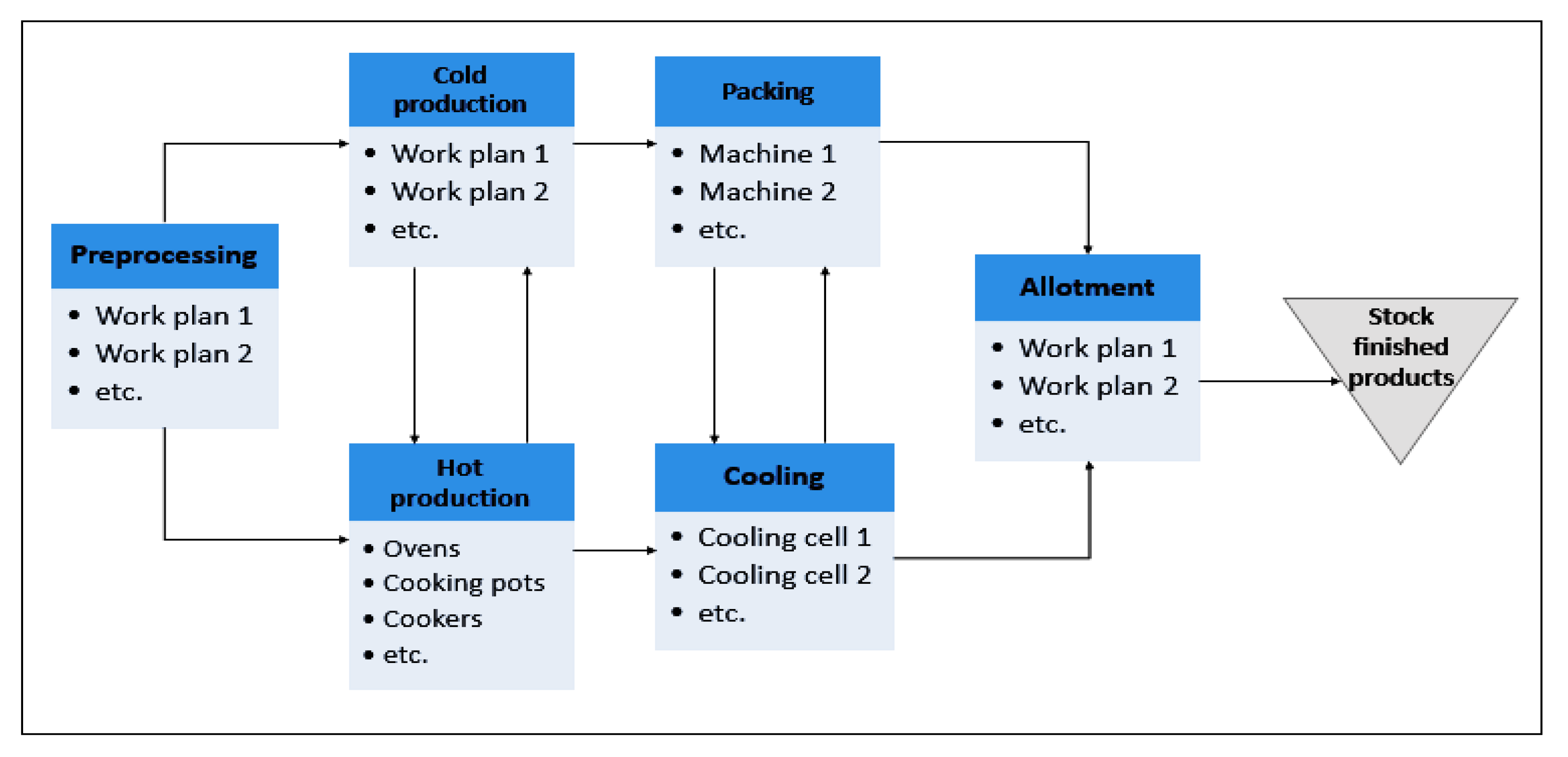
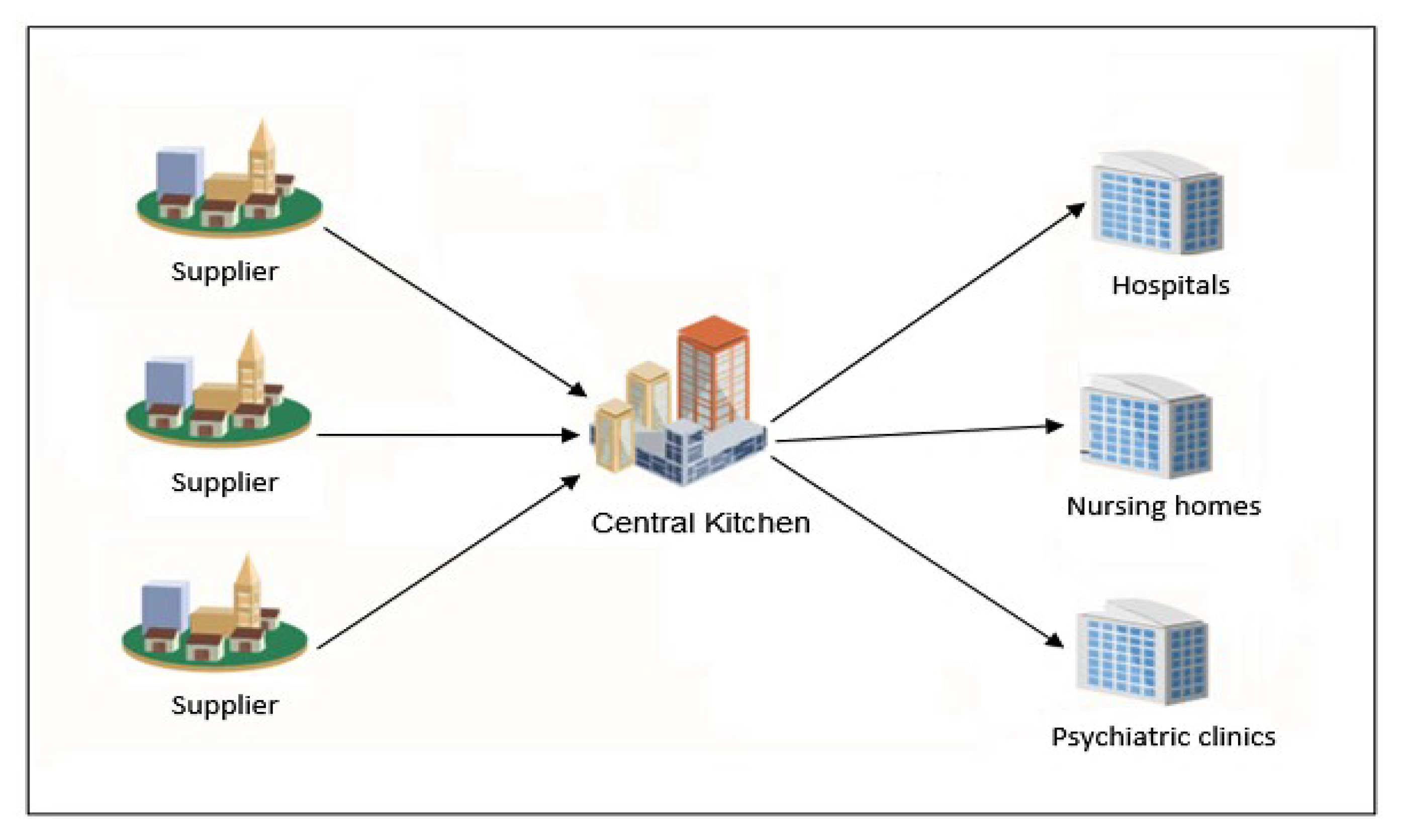
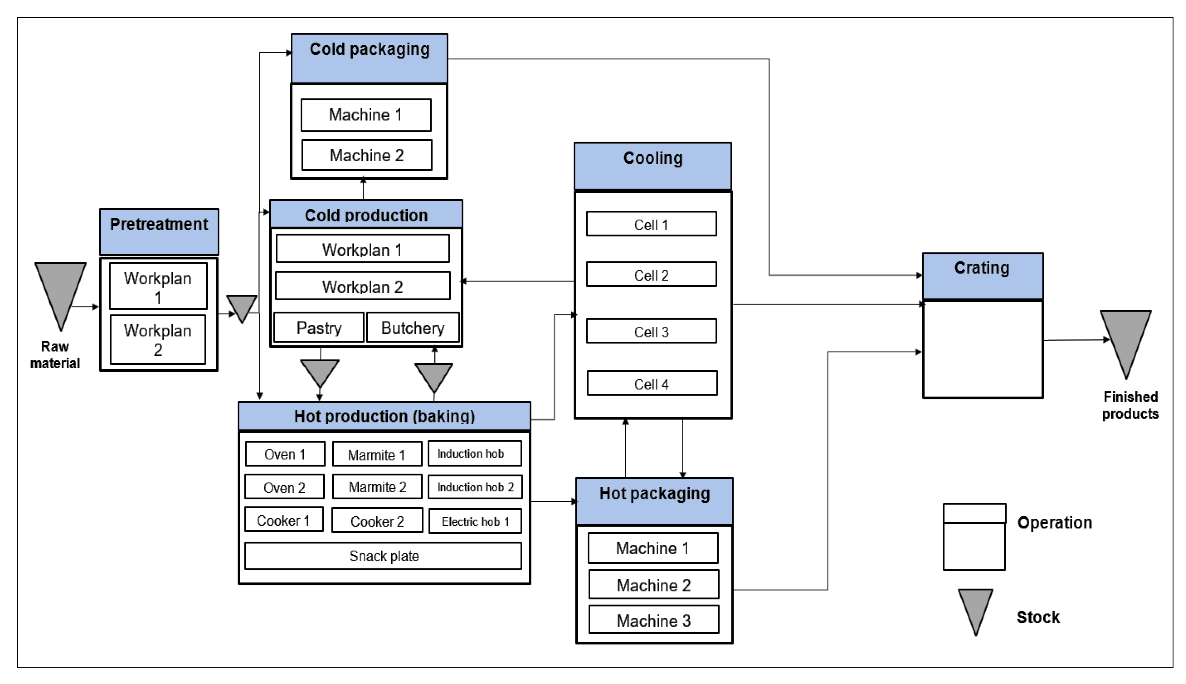
3. Problem Description

The problem of food production process scheduling considered in this study aims to schedule the operations from the pre-treatment of raw materials to the stock of finished products of a meal manufacturing process in hospital catering or, more generally, in collective catering. Figure 2 represents the typical production areas and the different material resources available for realizing the operations of the meal-making process. This problem is considered as a flexible job shop problem with sequence-dependent setup time and job splitting by integrating specific industrial constraints, such as the days of pre-treatment and production of products, the product delivery times, and the amounts of human and material resources available, in addition to the different constraints described below.

The addressed problem is considered as a flexible job shop scheduling problem with sequence-dependent setup time, since each job has its own order of operations and each operation has to be assigned to one among a set of possible machines. This problem can be described by a set of N jobs, where each job i corresponds to the preparation of a dish characterized by a number of portions $Q_i$ (quantity) and a set of operations $J_i$ for the preparation of the dish (from raw material to finished product). It is worth highlighting that the dishes to be prepared do not have the same order of operating ranges (set of operations necessary for the preparation of the dish). For each job, there is a due date $D_i$ to respect.

For each operation of an operating range, there is a set of material resources that are used to realize it, such as ovens, cooking pots, cookers, induction hobs, packaging machines, cooling cells (Figure 2). These material resources can be classified into three categories: $M_1$, $M_2$, and $M_3$. $M_1\subset M$ is composed of material resources with a capacity of one portion and that can not process several jobs at the same time (material resources that can perform preprocessing and cold production operations). The set $M_2\subset M$ represents the material resources with a capacity greater than one portion and that cannot process several jobs at the same time (ovens, etc.). $M_3\subset M$ correspond to the set of material resources with a capacity greater than one portion and that can process several jobs at the same time (cooling cells).

For each material resource, there is a setup time to take into account, which corresponds to the preparation time of the machine before carrying out an operation and the cleaning time of the machine between two consecutive operations. A time window of availability is known for each material resource.

Note that the corresponding machines may not be identical, involving different processing times according to the chosen machine. The setup times of machines are sequence dependent because they depends on the preceding operation on the same machine. The food production process scheduling involves two steps: (i) assignment of operations to machines and (ii) sequencing of operations on machines.

As mentioned previously, in order to respect the production capacities of material resources, a job can be split into smaller sub-lots in such a way that the operations of sub-lots of a job can be performed simultaneously on different machines. This strategy, which is useful when machine capacity does not allow the treatment of the whole job, also enables a more efficient processing scheme.

The criterion to minimize in the present study is the total flow time of jobs in the production system. The choice of this criterion is based on the fact that the respect of the cold chain at each stage of the product life cycle must be ensured. The aim is to constantly maintain a low temperature (positive or negative, depending on the product) to ensure the maintenance of all the food qualities (hygienic, nutritional, and gustatory).

4. Mathematical Model

In this section, a mixed-integer linear programming model is presented. This model formalizes and solves small-sized instances of the studied problem by using the Cplex solver. The solutions of the small-sized instances can be used to validate the efficiency of the developed metaheuristic methods.

4.1. Assumptions

The mathematical model for the scheduling of the food production process inherits its main assumptions from the standard flexible job shop scheduling problem with sequence-dependent setup times and additional features due to the job splitting:

• Jobs are independent of each other,
• A job can be split into sub-lots,
• The sub-lots of a job can be grouped on the machines to be treated at the same time,
• Each sub-lot of a job consists of a set of operations that must be processed consecutively (precedence constraints between operations of sub-lots of jobs),
• Each operation of a sub-lot has a given processing time,
• The preemption of operations of sub-lots of jobs is not allowed, i.e., operation processing on a machine cannot be interrupted,
• Each job has a given due date (finish date of production at latest),
• Sub-lot sizes (number of portions) are discrete,
• Sub-lots creation is consistent throughout the processing sequence, meaning that job splitting and sub-lot sizes remain constant for all operations,
• Machines are independent,
• A machine can process, at most, one operation of a job at the same time,
• The setup times of machines are dependent on the sequence of operations of sub-lots of jobs,
• Material resources have given availability time windows that must be taken into account.

Taking these assumptions into account, the objective is to find a schedule involving sub-lot assignments to machines and sub-lot sequencing for each machine in such a way that each job’s demand is fulfilled, different constraints of the problem are respected, and the total flow time of jobs in the production system is minimized.

4.2. Notations

The definition of the developed mathematical model’s parameters relies on the following sets and indexes:

• M: set of all material resources, where $m=\left|M\right|$.
• N: set of jobs (dishes to prepare), where $n=\left|N\right|$ and $\left\{0,n+1\right\}$ are two dummy jobs.
• $J_i$: set of operations of job $i\in N$, such that the operation $j\in J_i$ is done before the operation $j+1\in J_i$ and $|J_0|=|J_{n+1}|=1$.
• $Q_i$: number of portions (quantity) of job $i\in N$.
• $q_i$: number of portions in each sub-lot of job $i\in N$.
• $L_i$: set of sub-lots of job $i\in N$, with $|L_0|=|L_{n+1}|=1$ and $l_i=\left|L_i\right|$ such that $l_i=\lceil {\displaystyle \frac{Q_i}{q_i}}\rceil$.
• $d_i$: due date of job $i\in N$.
• $M_{ij}\subset M$: set of material resources that can perform the operation $j\in J_i$ of job $i\in N$.
• $R_k$: maximum capacity in number of portions of the material resource $k\in M$.
• $P_{ijk}^{{}^{\prime }}$: unit processing time of operation $j\in J_i$ of job $i\in N$ on the material resource $k\in M_1$.
• $P_{ijk}$: processing time of operation $j\in J_i$ of job $i\in N$ on the material resource $k\in M_2\cup M_3$.
• $s_{ijhgk}$: setup time of material resource $k\in M_{ij}\cap M_{hg}$ if the operation $j\in J_i$ of job $i\in N$ directly precedes the operation $g\in J_h$ of job $h\in N$ on the material resource $k\in M_{ij}\cap M_{hg}$.
• $T_k$: preparation time of the material resource k at the beginning of scheduling.
• $E_k$: cleaning time of the material resource k at the end of scheduling.
• $[A_k,Y_k]$: time window of availability of the material resource $k\in M$.
• B: big integer.

4.3. Decision Variables

• $X_{iljk}$: binary variable that equal to 1 if operation $j\in J_i$ of sub-lot $l\in L_i$ of job $i\in N$ is assigned to the material resource $k\in M_{ij}$, and 0 otherwise.
• $F_{iljh{l}^{\prime }gk}$: binary variable that is equal to 1 if operation $j\in J_i$ of sub-lot $l\in L_i$ of job $i\in N$ directly precedes operation $g\in J_h$ of sub-lot $l^{\prime }\in L_h$ of job $h\in N$ on the material resource $k\in M_{ij}\cap M_{hg}$, and 0 otherwise.
• $Z_{il{l}^{\prime }jk}$: binary variable that is equal to 1 if operation $j\in J_i$ of sub-lot $l\in L_i$ of job $i\in N$ starts and finishes at the same time as the operation $j\in J_i$ of sub-lot $l^{\prime }\in L_i$ of job $i\in N$ on the material resource $k\in M_{ij}$, and 0 otherwise.
• $S_{iljk}$: starting time of operation $j\in J_i$ of sub-lot $l\in L_i$ of job $i\in N$ on the material resource $k\in M_{ij}$.
• $C_{iljk}$: completion time of operation $j\in J_i$ of sub-lot $l\in L_i$ of job $i\in N$ on the material resource $k\in M_{ij}$.
• $C_i$: completion time of job $i\in N$.

4.4. Mathematical Model

In the literature, there exist different mathematical model formulations for the standard flexible job shop scheduling problem. The mathematical model proposed by Buddala and Mahapatra [31] takes into account constraints on processing times, precedence between operations, and machine capacity in number of operations processed at the same time, which corresponds with the studied problem. However, this model does not take into consideration the constraints on machine capacity in the number of portions, machine availability time windows, sequence-dependent setup time, due dates of jobs, splitting of jobs, and batching of sub-lots.

The developed mathematical model that integrates all these constraints is formulated as indicated through Equations (1) to (22):

$$\begin{array}{c}\hfill Min\sum _{i\in N}{C}_i\end{array}$$

(1)

$$\begin{array}{c}\hfill C_i\ge \sum _{k\in M_{ij}}{C}_{iljk},\forall i\in N,l\in L_i,j\in J_i\end{array}$$

(2)

$$\begin{array}{c}\hfill S_{iljk}+C_{iljk}\le B\ast X_{iljk},\forall i\in N,l\in L_i,j\in J_i,k\in M_{ij}\end{array}$$

(3)

$$\begin{array}{c}\hfill C_{iljk}-S_{iljk}\ge P_{ijk}-B\ast (1-X_{iljk}),\forall i\in N,l\in L_i,j\in J_i,k\in M_2\cup M_3\end{array}$$

(4)

$$\begin{array}{c}\hfill C_{iljk}-S_{iljk}\ge P_{ijk}^{\prime }\ast Q_i-B\ast (1-X_{iljk}),\forall i\in N,l\in L_i,j\in J_i,k\in M_1\end{array}$$

(5)

$$\begin{array}{c}\hfill S_{h{l}^{\prime }gk}\ge C_{iljk}+s_{ijhgk}-B\ast (1-F_{iljh{l}^{\prime }gk}),\forall i\in N,l\in L_i,j\in J_i,h\in N,l^{\prime }\in L_h,g\in J_h,\\ \hfill k\in M_{ij}\cap M_{hg}\backslash M_3\end{array}$$

(6)

$$\begin{array}{c}\hfill S_{i{l}^{\prime }jk}\ge C_{iljk}+s_{ijijk}-B\ast (1-F_{ilji{l}^{\prime }jk})-B\ast Z_{il{l}^{\prime }jk},\forall i\in N,l,l^{\prime }\in L_i,j\in J_i,k\in M_{ij}\cap M_{hg}\end{array}$$

(7)

$$\begin{array}{c}\hfill S_{iljk}-S_{i{l}^{\prime }jk}\le B\ast (1-Z_{il{l}^{\prime }jk}),\forall i\in N,l,l^{\prime }\in L_i,j\in J_i,k\in M_2\cup M_3\end{array}$$

(8)

$$\begin{array}{c}\hfill C_{iljk}-C_{i{l}^{\prime }jk}\le B\ast (1-Z_{il{l}^{\prime }jk}),\forall i\in N,l,l^{\prime }\in L_i,j\in J_i,k\in M_2\cup M_3\end{array}$$

(9)

$$\begin{array}{c}\hfill \sum _{h\in N\backslash \left\{0\right\}}\sum _{l^{\prime }\in L_h}\sum _{g\in J_h}{F}_{iljh{l}^{\prime }gk}=1,\forall i\in N\backslash \left\{n+1\right\},l\in L_i,j\in J_i,k\in M_{ij}\cap M_{hg}\end{array}$$

(10)

$$\begin{array}{c}\hfill \sum _{i\in N\backslash \left\{n+1\right\}}\sum _{l\in L_i}\sum _{j\in J_i}{F}_{iljh{l}^{\prime }gk}=1,\forall h\in N\backslash \left\{0\right\},l^{\prime }\in L_h,g\in J_h,k\in M_{ij}\cap M_{hg}\end{array}$$

(11)

$$\begin{array}{c}\hfill \sum _{k\in M_{ij}}{S}_{iljk}-\sum _{k\in M_{ij-1}}{C}_{ilj-1k}\ge 0,\forall i\in N,l\in L_i,j\in J_i\end{array}$$

(12)

$$\begin{array}{c}\hfill \sum _{k\in M_{ij}}{X}_{iljk}=1,\forall i\in N,l\in L_i,j\in J_i\end{array}$$

(13)

$$\begin{array}{c}\hfill C_i\le d_i,\forall i\in N\end{array}$$

(14)

$$\begin{array}{c}\hfill \sum _{l,l^{\prime }\in L_i}{q}_i\ast Z_{il{l}^{\prime }jk}\le R_k,\forall i\in N,j\in J_i,k\in M_2\cup M_3\end{array}$$

(15)

$$\begin{array}{c}\hfill S_{iljk}\ge A_k,\forall i\in N,l\in L_i,j\in J_i,k\in M_{ij}\end{array}$$

(16)

$$\begin{array}{c}\hfill C_{iljk}\le Y_k,\forall i\in N,l\in L_i,j\in J_i,k\in M_{ij}\end{array}$$

(17)

$$\begin{array}{c}\hfill Z_{il{l}^{\prime }jk}=0,\forall i\in N,l,l^{\prime }\in L_i,j\in J_i,k\in M_1\end{array}$$

(18)

$$\begin{array}{c}\hfill X_{iljk}\in \{0,1\},\forall i\in N,l\in L_i,j\in J_i,k\in M_{ij}\end{array}$$

(19)

$$\begin{array}{c}\hfill Z_{il{l}^{\prime }jk}\in \{0,1\},\forall i\in N,l,l^{\prime }\in L_i,j\in J_i,k\in M_{ij}\end{array}$$

(20)

$$\begin{array}{c}\hfill S_{iljk}\ge 0,C_{iljk}\ge 0,C_i\ge 0,\forall i\in N,l\in L_i,j\in J_i,k\in M_{ij}\end{array}$$

(21)

$$\begin{array}{c}\hfill F_{iljh{l}^{\prime }gk}\in \{0,1\},\forall i\in N,l\in L_i,j\in J_i,h\in N,l^{\prime }\in L_h,g\in J_h,k\in M_{ij}\cap M_{hg}.\end{array}$$

(22)

In the mathematical model presented previously, Equation (1) represents the objective function, which consists in minimizing the total flow time of jobs in the production system. It is defined as the sum of the completion times of all jobs since the release dates are equal to zero. The completion times of jobs are computed as the completion time of the last sub-lot derived from the considered job, as indicated in Equation (2). Note that, due to Equation (3), for given $i\in N$, $l\in L_i$, and $j\in J_i$, variables $S_{iljk}$ and $C_{iljk}$ are equal to zero if the machine $k\in M_{ij}$ is not chosen to realize the operation of the considered sub-lot. On the other hand, when $X_{iljk}$ is equal to 1, Equations (4) and (5) activate the relationship between the starting time and completion time of an operation of a sub-lot. In this case, the processing time does not depend on the quantity of jobs for the material resources $M_2\cup M_3$ (Equation (4)), but it depends on the quantity of jobs for the material resources $M_1$ Equations (5) and (6) consider sequence-dependent setup times between the completion time and starting time of two operations of sub-lots that are processed on a machine one after another. Equation (7) disable Equation (6) if two different sub-lots of the same job are performed at the same time by the same material resource. Equations (8) and (9) require that if two operations of two different sub-lots of the same job are assigned at the same time to a material resource $M_2$ or $M_3$, they must have the same respective starting time and completion time. Equation (10) ensure that only one operation immediately follows the jth operation of sub-lot $l\in L_i$ of job $i\in N$ on machine $k\in M_{ij}\cap M_{hg}$, and Equation (11) guarantee that only one operation immediately precedes the gth operation of sub-lot $l^{\prime }\in L_h$ of job $h\in N$ on machine $k\in M_{ij}\cap M_{hg}$. Equation (12) establishes the precedence constraints between two consecutive operations of the same sub-lot. Equation (13) enforce that each operation of each sub-lot should be assigned to exactly one machine among the possible ones. The respect for the due dates of jobs is modeled by Equation (14). Equation (15) ensure that the capacities of material resources in the number of portions are respected. The respect for time windows of availability of material resources is modeled by Equations (16) and (17). Finally, Equations (19)–(22) define the domain of the decision variables.

4.5. Computational Results of the Mathematical Model

The mathematical model presented previously was implemented in the Java programming language using the Cplex library. This mathematical model was tested on 150 instances of different types: real instances of the hospital center of Troyes (HCT), randomly generated instances of the HCT type, randomly generated instances, and instances adapted from the literature (Sriboonchandr et al. [32], Nouri et al. [33], Azzouz et al. [34], Mousakhani [26], Lee et al. [35], Bagheri and Zandieh [25], Pezzella et al. [36]). The details of the results of these different types of instances are presented in Section 6. The mathematical model was able to find solutions in less than three hours of execution for the small instances with less than eight jobs, 10 sub-lots, 39 operations, and 29 machines. The execution times of the mathematical model for these instances varied according to the number of jobs, sub-lots, and operations. The computational results of the proposed mathematical model for different types of instances and, specifically, for real instances of HCT show the limits of an exact resolution for the problem of scheduling of the food production process.

5. Resolution Methods

5.1. Genetic Algorithm

Solving the flexible job shop problem is known to be strongly NP-hard (Xia and Wu [37], Fattahi et al. [38]). The introduction of sequence-dependent setup time and job splitting complicates the already difficult flexible job shop problem. In order to solve this problem efficiently, we developed a hybrid method that combines a genetic algorithm and three local research methods. The elements of this hybrid method are presented in the following subsections.

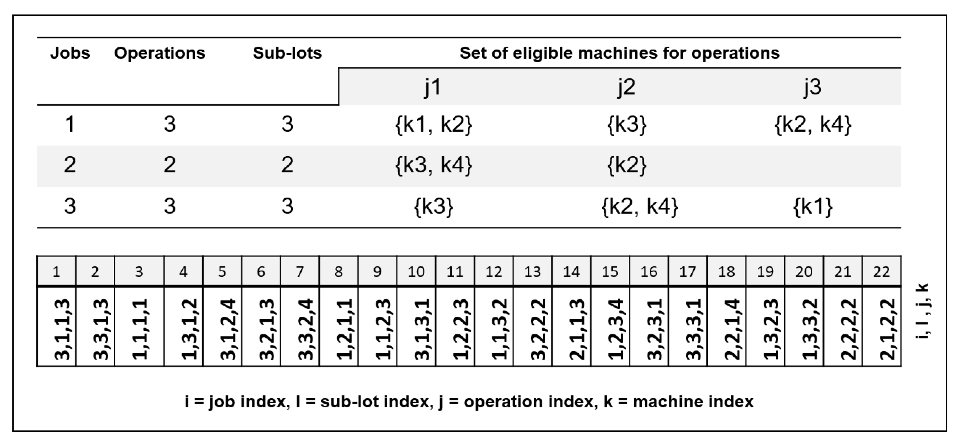
5.1.1. Solution Representation

By solving a flexible job shop scheduling problem using a genetic algorithm, Kacem [39] used a solution representation by coding both the assignment and the sequencing of operations on different machines. A similar representation is used in this paper to solve the flexible job shop scheduling problem with job splitting by considering each sub-lot as a job. To illustrate this representation, let us consider a small example with three jobs and four machines. The numbers of operations of sub-lots for each job and all the machines eligible for each operation are given in Figure 3. A representation of the assignment of operations to machines and their sequencing is coded in a chromosome, as shown in Figure 3. In this chromosome, each gene is represented by a quadruple $(i,l,j,k)$, designating the assignment of operation j of sub-lot l of job i to machine k. The sequence of genes in the chromosome represents the sequence of operations on machines. The chromosome decoding procedure is carried out by reading it from left to right. For example, the assignment and sequencing of operations on machine 1 can be decoded as follows: $(1,1,1,1)$→$(1,2,1,1)$→$(3,1,3,1)$→$(3,2,3,1)$→$(3,3,3,1)$. This information is obtained from genes 3, 8, 10, 16, and 17 in the chromosome, where $k=1$. In this chromosome, for a given i and l, the gene $(i,l,j,k)$ is always located on the right of all the other genes $(i,l,j,k^{\prime })$ with $j^{\prime }<j$. This ensures that the precedence requirements of the operations of a particular sub-lot are not violated.

5.1.2. Initial Population

The initial population plays an important role in the performance of genetic algorithms. An initial population with great diversity between solutions can avoid falling into a premature convergence or a local minimum. Different assignment and sequencing rules were used to achieve the diversity of solutions:

• Random assignment (RA): The operations are randomly assigned to machines.
• SPT assignment (SPTA): For each operation, the machine with a smaller processing time is selected to perform this operation.
• LPT assignment (LPTA): For each operation, the machine with a longer processing time is selected to perform this operation.
• Minimum machine workload assignment (MMWA): The operations are iteratively assigned to machines based on their processing times and machine workloads. The workload of a machine depends on its type. For the set of machines $M_1$, the workload is the sum of processing times of operations assigned to the machine. For the set of machines $M_2$ and $M_3$, the workload is the total machine occupation time. The procedure consists in finding the machine with the minimum workload for each operation.
• Random sequence (RS): This heuristic randomly orders the operations on each machine.
• SPT sequence (SPTS): Operations with the shortest processing time will be processed first.
• Most number of operations Remaining (MNOR): This heuristic consists of processing the operations of the sub-lot of the job that has the most operations remaining as a priority.
• Most work remaining (MWR): The operations that have the most remaining processing time will be prioritized for processed.

For the construction of the initial population using the heuristics described above, the procedure consists of randomly choosing an assignment and a sequencing heuristic and building solutions, such as the constraints of precedence between the operations of sub-lots of jobs, the due dates of jobs, the time windows of availability of material resources, and the respect for the production capacities of machines.

5.1.3. Fitness Evaluation

Algorithm 1 decodes the chromosomes to obtain the objective function value and a workable representation of the solutions.

Algorithm 1: Evaluation steps of the fitness function of a chromosome

Step 01: Set $p=1$. Step 02: Set $i,l,j,k$, the index values of the gene located at the P position of the chromosome. Step 03: Calculate the completion time $C_{iljk}$. If operation j of sub-lot l of job i is the first operation assigned to the machine k and $j=1$, $$\begin{array}{c}\hfill S_{iljk}=A_k+T_k;C_{iljk}=S_{iljk}+P_{ijk};C_i=Max\{C_i,C_{iljk}\}\end{array}$$ If operation j of sub-lot l of job i is the first operation assigned to the machine k, $j>1$, and the operation $j-1$ is assigned to the machine $k^{\prime }$, $$\begin{array}{c}\hfill S_{iljk}=Max\{A_k+T_k,C_{ilj-1k^{\prime }}\};C_{iljk}=S_{iljk}+P_{ijk};C_i=Max\{C_i,C_{iljk}\}\end{array}$$ If operation $j^{\prime }$ of sub-lot $l^{\prime }$ of job $i^{\prime }$ is the operation to be processed immediately before the operation j of sub-lot l of job i on the machine k and $j=$ 1, $$\begin{array}{c}\hfill S_{iljk}=s_{i^{\prime }{j}^{\prime }ijk}+C_{i^{\prime }{l}^{\prime }{j}^{\prime }k};C_{iljk}=S_{iljk}+P_{ijk};C_i=Max\{C_i,C_{iljk}\}\end{array}$$ If operation j of sub-lot l of job i and the operation j of sub-lot $l^{\prime }$ of job i are assigned to the machine k and $j=1$, If ($k\in M_2\cup M_3$ and $2\ast q_i<=R_k$) $$\begin{array}{c}\hfill S_{iljk}=S_{i{l}^{\prime }jk};C_{iljk}=S_{iljk}+P_{ijk};C_i=Max\{C_i,C_{iljk}\}\end{array}$$ If ($k\in M_2\cup M_3$ et $2\ast q_i>R_k$) ou ($k\in M_1$) $$\begin{array}{c}\hfill S_{iljk}=F_{i{l}^{\prime }jk};C_{iljk}=S_{iljk}+P_{ijk};C_i=Max\{C_i,C_{iljk}\}\end{array}$$ If operation $j^{\prime }$ of sub-lot $l^{\prime }$ of job $i^{\prime }$ is the operation to be processed immediately before the operation j of sub-lot l of job i on the machine k, $j>1$, and the operation $j-1$ is assigned to the machine $k^{\prime }$, $$\begin{array}{c}\hfill S_{iljk}=Max\{s_{i^{\prime }{j}^{\prime }ijk}+C_{i^{\prime }{l}^{\prime }{j}^{\prime }k},C_{ilj-1k^{\prime }}\};C_{iljk}=S_{iljk}+P_{ijk};C_i=Max\{C_i,C_{iljk}\}\end{array}$$ If operation j of sub-lot l of job i and the operation j of sub-lot $l^{\prime }$ of job i are assigned to the machine k, $j>1$, and the operation $j-1$ is assigned to the machine $k^{\prime }$, If ($k\in M_2\cup M_3$ and $2\ast q_i<=R_k$) $$\begin{array}{c}\hfill S_{iljk}=S_{i{l}^{\prime }jk};C_{iljk}=S_{iljk}+P_{ijk};C_i=Max\{C_i,C_{iljk}\}\end{array}$$ If ($k\in M_2\cup M_3$ and $2\ast q_i>R_k$) or ($k\in M_1$) $$\begin{array}{c}\hfill S_{iljk}=Max\{C_{i{l}^{\prime }jk},C_{ilj-1k^{\prime }}\};C_{iljk}=S_{iljk}+P_{ijk};C_i=Max\{C_i,C_{iljk}\}\end{array}$$ Step 04: If p is less than the total number of operations of sub-lots of jobs, increment its value by 1 and go to Step 2; otherwise, go to Step 05. Step 05: Calculate the fitness function of the solution by using the equation ${\sum }_i{C}_i$.

It is worth noting that for a given i and l, the gene $(i,l,j,k)$ is always located on the right of all the other genes $(i,l,j^{\prime },k^{\prime })$ with $j^{\prime }<j$. Based on this property, when the completion time of operation $(i,l,j,k)$ on machine k is to be calculated, the completion time of operation $(i,l,j-1,k^{\prime })$ is already calculated and available, regardless of the machine to which this preceding operation is assigned. Moreover, the completion time of the operation $(i^{\prime },l^{\prime },j^{\prime },k)$ to be processed on machine k immediately before operation $(i,l,j,k)$ is also calculated and available.

Genetic operators evolve the population to promising regions of the research space. The convergence behavior of the algorithm depends largely on them. These operators are generally categorized as selection, crossover, and mutation operators.

5.1.4. Selection Operator

The process of selecting two parents from the population for reproduction is called selection. The aim of the selection operator is to highlight individuals with the best fitness in hopes that their resulting offspring are more fit individuals. In the proposed genetic algorithm, we used the two-way tournament selection operator introduced in [40]. The selection operator is involved in holding competitions among randomly selected individuals and choosing the one with the best fitness (smallest total flow time). This individual is added to a mating population, which is used to form the next generation. Then, the individuals in the tournament are placed back in the current population, and the process is repeated until the number of individuals added to the mating population is equal to the population size.

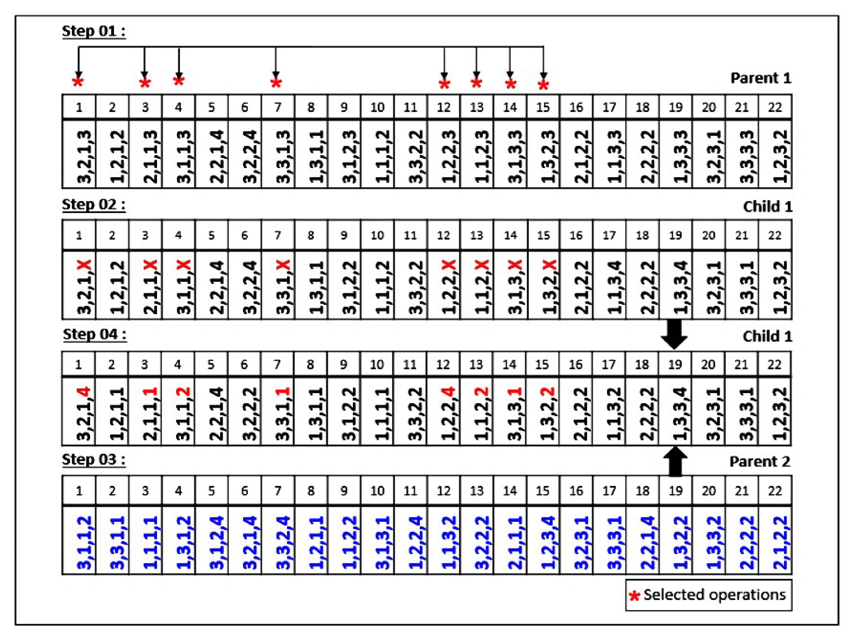
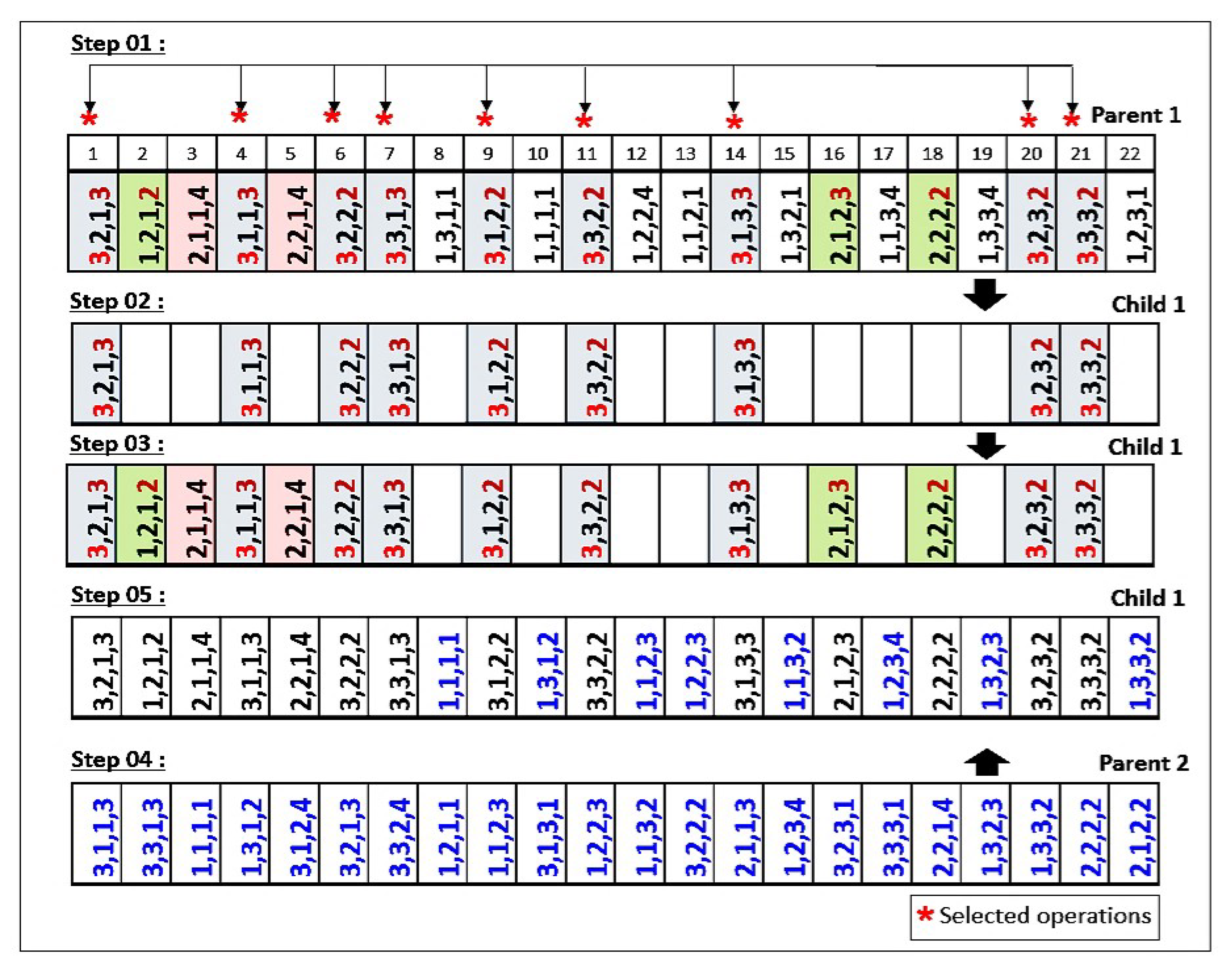
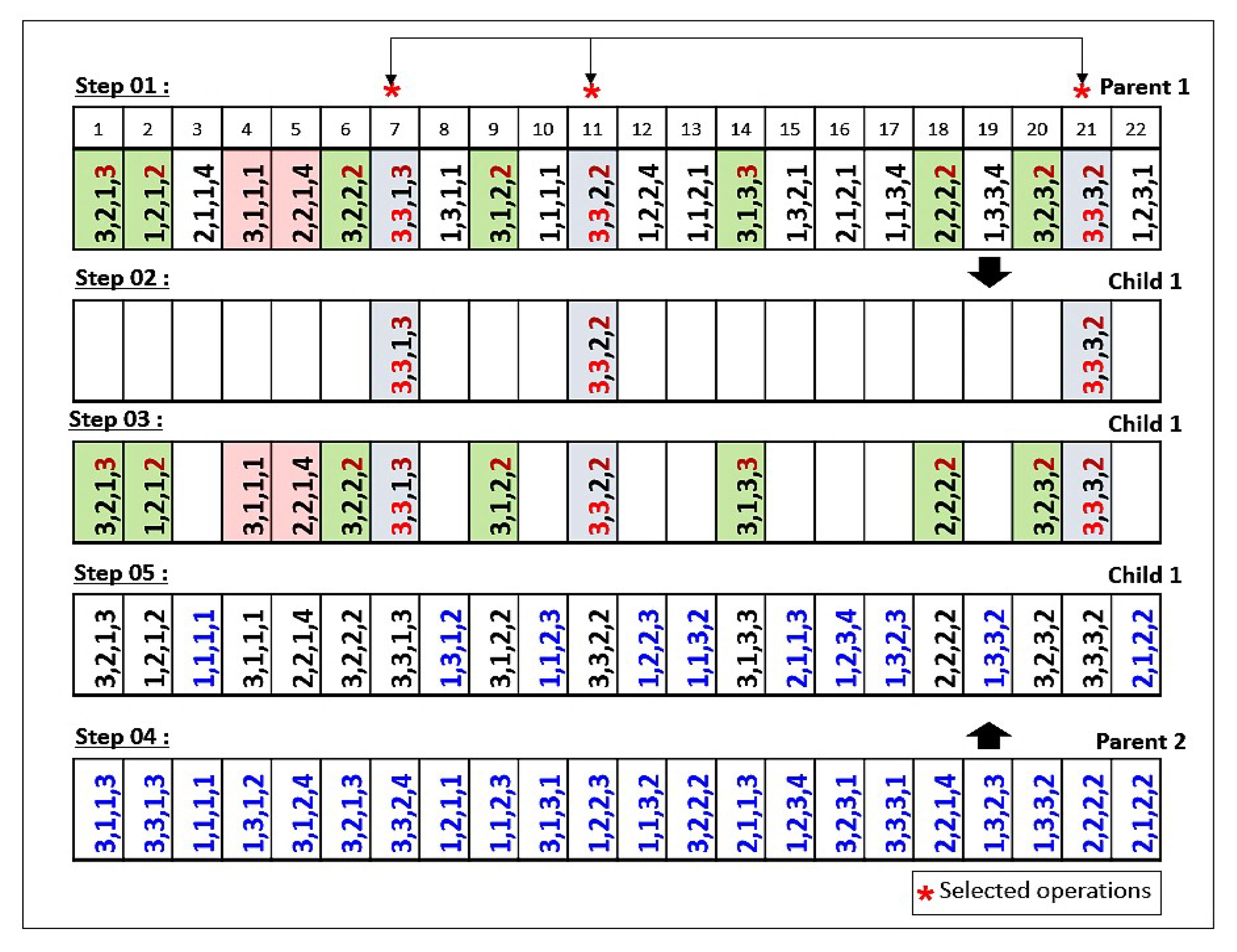
5.1.5. Crossover Operator

After the selection of chromosomes for reproduction, a crossover operator is applied to combine the features of the parent chromosomes in order to produce a new child. The individuals in the mating population are randomly paired to create child individuals. For two parents, the algorithm arbitrarily selects one of the available crossover operators and applies it with a certain probability to create two child individuals by exchanging information contained in the parent chromosomes.

Different crossover operators are proposed and can be categorized as assignment or sequence crossover operators. The assignment crossover operators consist of generating offsprings by exchanging the assignment of operations to machines in the parent chromosomes. The role of sequence crossover operators is to produce two new offspring by exchanging partial information of the sequences of operations on machines in the parent chromosomes. The assignment and sequence crossover operators developed in the proposed genetic algorithm are: OMAC (operation to machine assignment crossover), JLOSC (job-level operation sequence crossover), and SLOSC (sub-lot-level operation sequence crossover).

From a given pair of parent chromosomes, OMAC creates two child chromosomes, preserving the sequence of operations in each parent chromosome and modifying the machines’ affectation. The creation of a child chromosome using an OMAC crossover operator is illustrated in Figure 4. We assume that in the first step, the operations located in genes 1, 3, 4, 7, 12, 13, 14, and 15 are selected from parent 1 to change their assignments. Then, the second step is to copy all the genetic information of parent 1 to the offspring, except for the assignment information of the selected operations. The final step is to obtain the assignment information of the selected operations from parent 2 and then copy them to the corresponding genes in the offspring to produce a new child chromosome. The same process is repeated to create child 2 by starting to select the operations from the chromosome parent 2. Three versions of OMAC were developed to correspond to different ways of selecting the operations for which the assignment will be modified:

• OMAC 1: A set of operations of a sub-lot of jobs is chosen randomly.
• OMAC 2: A set of operations of sub-lots assigned to the loaded machines is selected.
• OMAC 3: A set of operations of sub-lots of jobs with larger completion times is chosen.

The objective of the crossover operator OMAC 2 is to balance the workload between the machines, whereas the goal of the crossover operator OMAC 3 is to reduce the ending dates of jobs with longer completion times.

The crossover sequencing operators JLOSC and SLOSC produce two new offspring by exchanging the sequencing information of parent chromosomes while keeping the assignment of machines in a gene unmodified. They are applied with given probabilities. The creation of the child chromosome by JLOSC and SLOSC with the preservation of the assignment information of parent chromosomes is illustrated in Figure 5 and Figure 6. In the JLOSC crossover operator, the first step is to select a set of operations from parent 1. The next step is to copy all of the genetic information of the genes that are associated with the chosen operations to the offspring. The final step is to fill the empty genes in the offspring chromosome, while the machine assignment information of the empty genes is preserved from parent 1. This is done by copying the remaining operations from parent 2 to the empty genes, while the operations retain their appearance order from the second parent. The same procedure is repeated to create child 2 by starting to select the operations from parent 2. SLOSC is identical to JLOSC, with a difference in the second step of SLOSC: Only the genetic information of the chosen genes with the same sub-lot and job indexes is copied to the offspring. Two operators of each kind were developed (JLOSC1, JLOSC2, SLOSC1, and SLOSC2):

• JLOSC1 and SLOSC1: The operations are chosen randomly.
• JLOSC2 and SLOSC2: The operations are chosen according to specific rules that consist of choosing the operations of jobs with smaller completion times.

The SLOSC1 operator is similar to the JLOSC1 operator, but instead of keeping the unmodified operations of all the sub-lots, only the information from the sub-lot of the selected operation is kept and copied to the child chromosome.

The SLOSC2 crossover operator is similar to the JLOSC2 crossover operator except that in the first step, a set of sub-lots of jobs with smaller completion times is chosen. The goal of the JLOSC2 and SLOSC2 crossover operators is to keep the sequencing of operations of jobs and the sequencing of operations of sub-lots of jobs, respectively, with smaller completion times.

It is important to note that, after the application of any crossover operator, in the child chromosome, for a given i and l, the gene $(i,l,j,k)$ is located after any gene $(i,l,j^{\prime },k^{\prime })$, where $j^{\prime }<j$. This ensures that precedence constraints between operations of a particular sub-lot are not violated in the new created child chromosome.

5.1.6. Mutation Operator

The role of mutation operators is to prevent the algorithm from being trapped in a local optimum and to maintain genetic diversity in the population. The mutation operators are usually applied on chromosomes with given probabilities. Assignment and sequence operators also exist amongst the mutation operators. Assignment mutation operators change the assignment of operations to machines without changing the sequencing of these operations, and sequence operators only change the sequencing property of the chromosome undergoing the mutation, while the assignment property is preserved. The mutation operators used in the developed genetic algorithm are:

• ROAM (random operation assignment mutation): This operator is applied with a given probability on a set of operations of a given individual chromosome and randomly changes the assignment property of these operations to another machine.
• OSSM (operation sequence shift mutation): Whenever OSSM is applied on an individual, a set of operations is selected. Then, these operations are moved to other positions on the chromosome in such a way that no precedence constraint is violated.

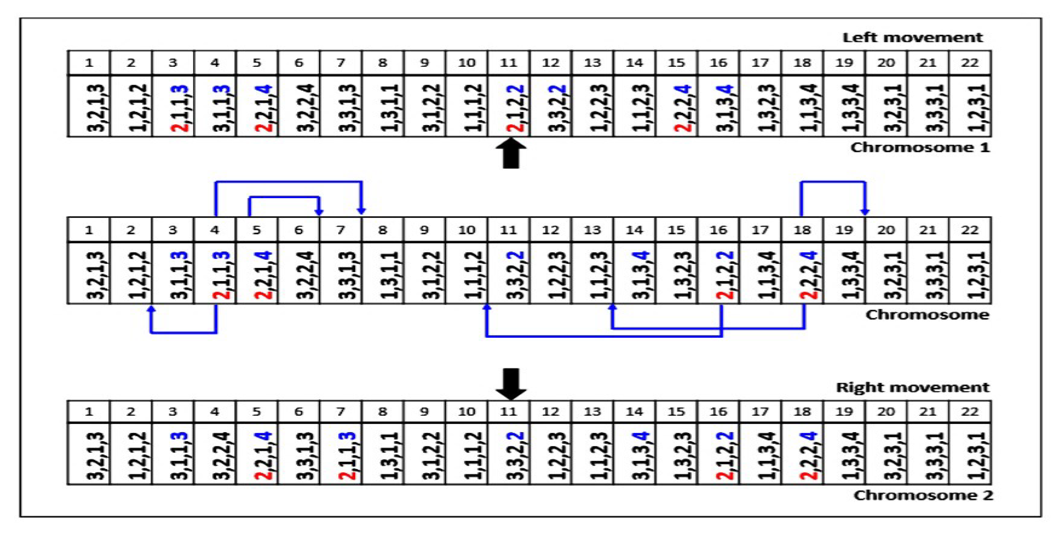
5.1.7. Local Search Methods

Local Search through Gene Movement

This local search method improves the quality of any solution built after the application of the crossover and mutation operators. It is repeated as long as the quality of solutions obtained is not improved. The procedure for this method is illustrated through an example in Figure 7. The first step is to choose a set of operations of jobs with longer completion times; the goal is to reduce these completion times. In the second step, the procedure performs a search in the neighborhood of a solution by changing the positions of the operations chosen on the machines in order to improve the quality of this solution. This process is repeated until the iteration criteria are met. The steps of this local search method are as follows:

• Step 01: Choose a set of operations of jobs with larger completion times in the current chromosome.
• Step 02: Each operation chosen in Step 01 is positioned just before the previous operation assigned to the same machine (left movement) or just after (right movement) the following operation assigned to the same machine, while respecting the constraints of precedence between operations of sub-lots of jobs. This process allows one to lead research in the neighborhood of a solution by changing the sequencing of operations on the machines.
• Step 03: This process is repeated until the maximum number of iterations is not reached.

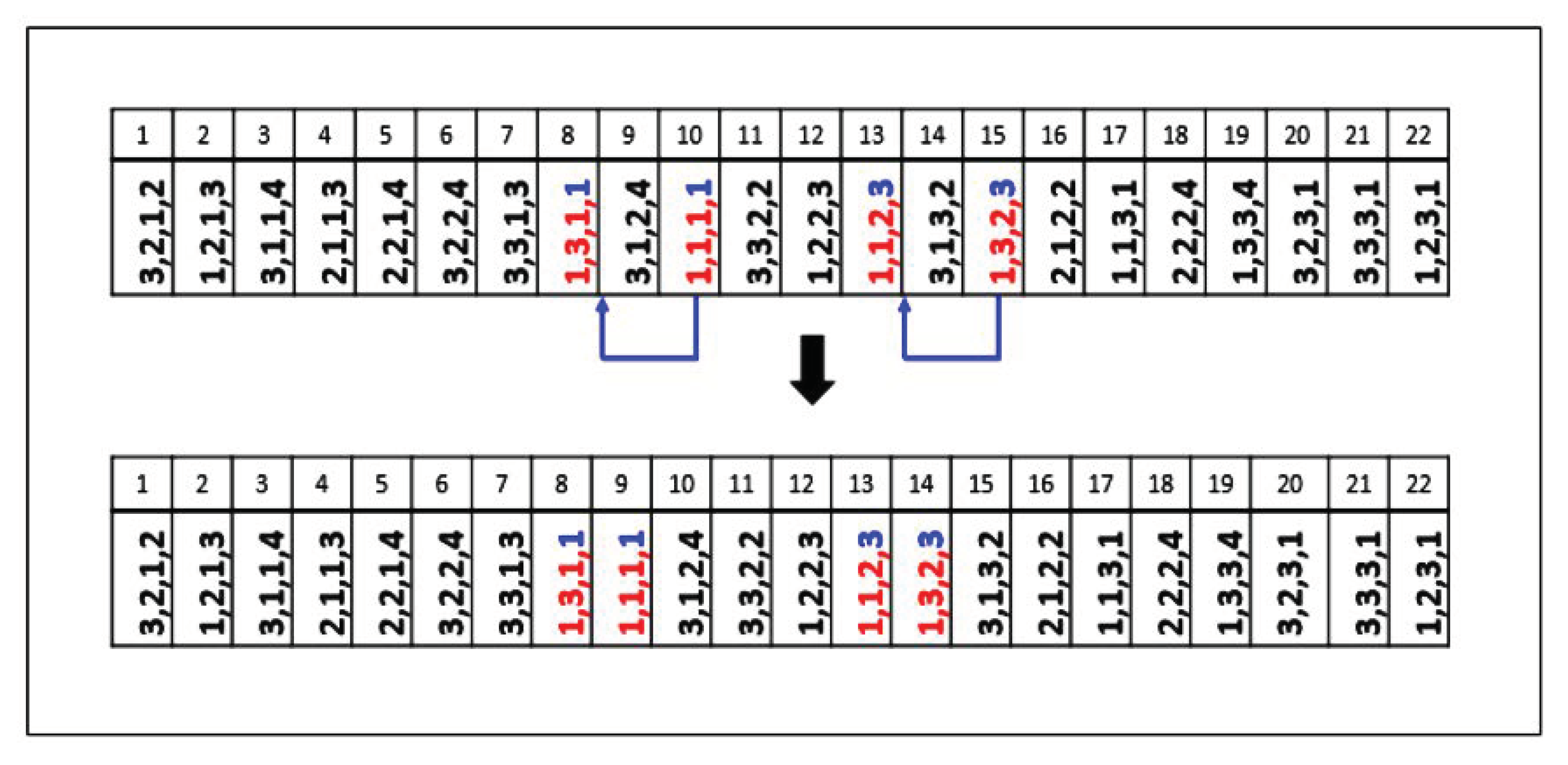
Local Search by Grouping Sub-Lots

This local search method consists of grouping the operations of sub-lots of jobs on machines if the capacities of the machines allow the processing of several operations at the same time. This method can only be applied for machines such as ovens and cooling cells. The procedure for this local search method is illustrated through an example in Figure 8. For each gene, the sub-lot grouping procedure consists of browsing the chromosome from left to right. If the sub-lots of the same job as the considered gene are assigned to the same machine and the latter can process several sub-lots at the same time, all the genes of these sub-lots are repositioned one next to the other in the chromosome, which means that these sub-lots are treated at the same time by the same machine. The grouping of operations of sub-lots of jobs on machines must take into account the precedence between operations of these sub-lots.

Local Search through Intelligent Assignment of Operations

In this local search approach, a set of operations assigned to the most loaded machines is reassigned to the least loaded compatible ones.

Table 2. Common and different elements between the two genetic algorithms.

	Initial Population	Crossover Operators	Mutation Operators
GA1	MMWA, SPT	OMAC1, JLOSC1, SLOSC1	ROAM, IOAM, OSSM
GA2	MMWA, MNOR	OMAC2, OMAC3, JLOSC2, SLOSC2	ROAM, IOAM, OSSM

gives the common and different elements between the two developed algorithms. In this table, the heuristics for the generation of the initial population, crossover, and mutation operators of the two genetic algorithms are given. The two algorithms differ in the generation methods of the initial population and in the crossover operators. In both algorithms, several affectation and sequence heuristics were tested for the generation of the initial population. In Table 2, the heuristics allowing one to obtain the best solutions are given. The crossover operators of the first genetic algorithm are based on random choices of operations, while in the second algorithm, different operators that are specific and more adapted to the studied problem have been developed. Regarding the mutation operators, they are common between the two algorithms. The pseudocode of the generic genetic algorithm is given in Algorithm 2.

Algorithm 2: Genetic algorithm

1. Initialization: The initial solutions are chosen using the heuristics described above; 2. Evaluation: Evaluation of the initial solutions using the procedure of fitness function computation;     nbIterations ← 0; nbIndividuals ← 0; 3. Application of the selection operator to choose the parent chromosomes to cross and mutate; 4. Randomly choose one of the crossover operators; 5. Application of the crossover operator chosen in 4; 6. Randomly choose one of the mutation operators; 7. Application of the mutation operator chosen in 6; 8. Application of the local search by grouping sub-lots on child chromosomes obtained after crossover and mutation; 9. nbIndividuals ← nbIndividuals + 1; 10. If the population size is reached, then go to 11, else go to 3; 11. Sorting solutions of the current population in ascending order of fitness functions; 12. Construction of the new population with solutions of the previous population; 13. Application of the local search methods through gene movement and intelligent assignment of operations on the $\alpha$ best solutions of the new population; 14. nbIterations ← nbIterations + 1; 15. If the maximum number of iterations is not reached, then go to 3, else go to 16; 16. End of algorithm

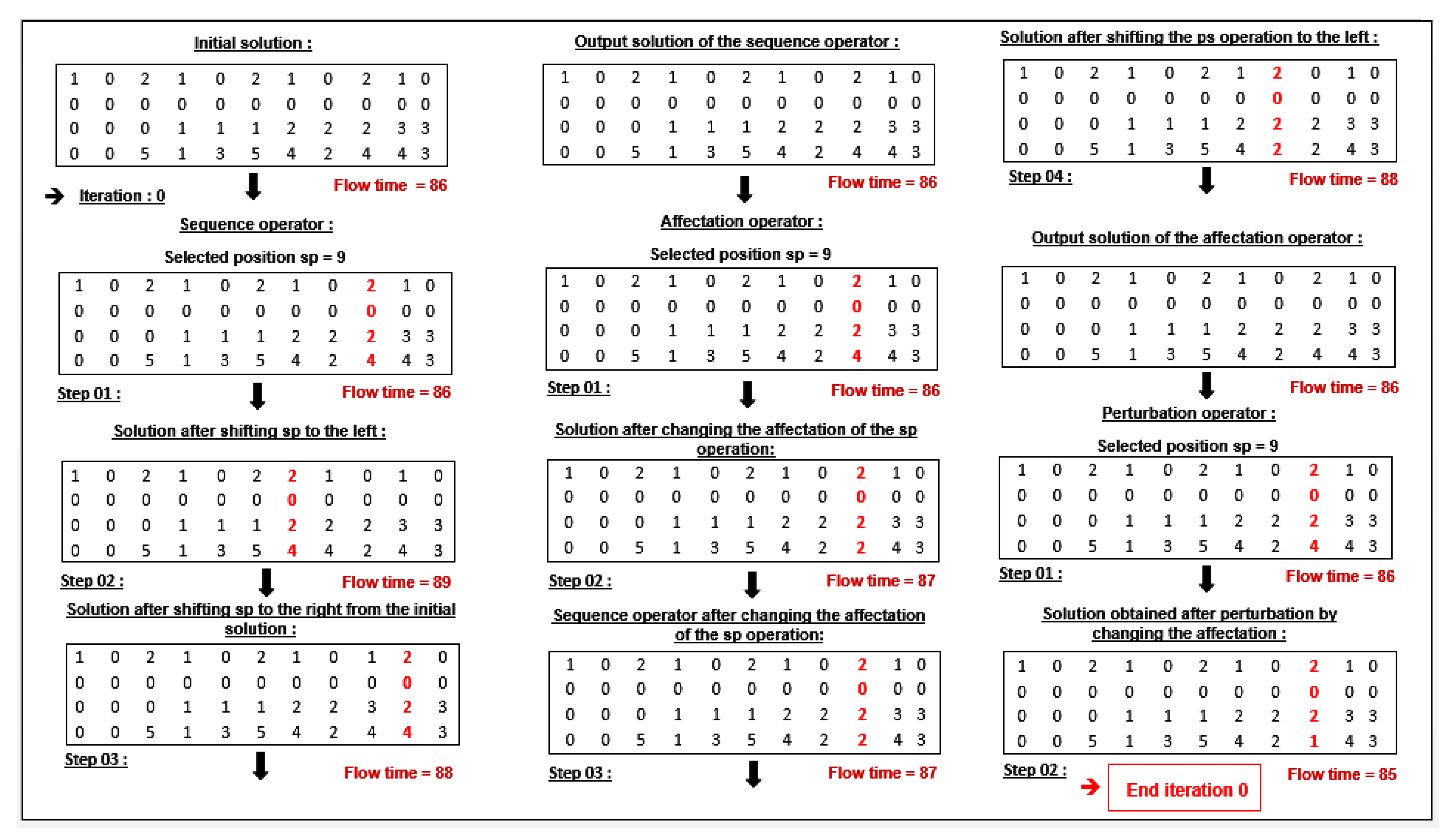
5.2. Iterated Local Search Algorithm

This section describes an iterated local search (ILS) algorithm for solving the studied problem. ILS is a simple, robust, and highly effective local search procedure that explores local optima in a given neighborhood (Lourenço et al. [41]).

The iterated local search algorithm starts from an initial solution and obtains a local optimum in its neighborhood through a local search procedure. To improve upon the current local optimum, ILS applies perturbation operators to this solution in order to move away from the current local optimum. An acceptance criterion is employed to determine which local optimum will become the current local optimum in the next iteration. The above process is repeated until a termination criterion is satisfied.

To generate the initial solutions of the iterative local search algorithms, the affectation and sequence heuristics for the generation of the initial population of the genetic algorithm are used, except that in the ILS algorithm, only one solution is generated.

The local search procedure is based on two operators: the affectation operator (AO) and sequence operator (SO). The affectation operator changes the assignment of a set of operations to the machines without changing their sequencing on the machines, while the sequence operator changes the sequencing of operations without changing their affectation to to machines.

Three affectation operators, AO1, AO2, and AO3, and three sequence operators, SO1, SO2, and SO3, were developed:

• AO1 and SO1: The operations are chosen randomly.
• AO2, AO3, SO2, and SO3: The operations are chosen according to rules developed to be specific to the studied problem.

The goal of the AO2 operator is to balance the workload between the machines, while AO3, SO2, and SO3 operators allow the reduction of the ending dates of jobs with larger completion times. The difference between these operators is in the choice of operations to change their assignments and sequences.

The first step of the SO operator consists of randomly choosing one of the sequence operators. Then, a set of operations in the current solution to be improved is chosen. The second step is to shift the selected operations to the left until the permutation of these operations with the previous operations assigned to the same machines is effective. If the left shift is blocked (precedence constraints are violated), then, from the solution obtained in the second step, the selected operations are shifted to the right until the permutation of these operations with the next operations assigned to the same machines is effective. This process is repeated until the maximum number of iterations is not reached.

In the AO operator, the first step is to choose one of the assignment operators. Then, a set of operations in the current solution to be improved is chosen. In the second step, the selected operations are assigned to another machine among a set of alternative machines. If the solution obtained after the reassignment of operations is not better than the current solution, then an SO sequence operator is applied on the selected operations with the new machine assignments obtained in the second step. This process is repeated for a given number of iterations.

The local search method can get stuck in a local optimum if the solution space is reduced. To fix this problem, a number of insertion moves to the current local optimum to obtain a perturbation solution are carried out. To determine the appropriate number of perturbations, different strategies have been tested. The best strategy, and that which is used in the algorithm, consists of performing a perturbation if the degree of similarity between the solutions is lower than a given threshold defined beforehand, which ensures a sufficient distance between solutions. The evaluation of the degree of similarity is based on the gaps between solutions. The similarity measures between solutions are evaluated to ensure the stability in the proposed solutions for the production scheduling.

The different steps of the iterative local search method in one iteration are illustrated through an example in Figure 9. The algorithm begins by generating an initial solution using one of the assignments and sequencing heuristics. Then, one of the SO sequence operators is applied. If no improvement of the solution is obtained after the application of the SO operator, the next step consists of applying an AO assignment operator on the operation chosen beforehand. If the application of the AO operator does not improve the initially generated solution, an SO operator with the new affectation obtained after the application of the AO operator is applied. If the solution is still not improved, a perturbation operator is applied on this solution, and the algorithm moves on to the next loop iteration. This operator consists of applying one of the randomly chosen sequencing or assignment operators. This process is repeated until the maximum number of perturbations is not reached.

Table 3. Common and different elements between the two iterated local search algorithms.

	Initial Solution	Sequence Operators	Affectation Operators
ILS1	SPT, MNOR	SO1	AO1
ILS2	MMWA, MNOR	SO2, SO3	AO2, AO3

gives the common and different elements between the two developed algorithms. In this table, the heuristics for the generation of initial population, affectation, and sequence operators of the two iterated local search algorithms are given. The difference between the two algorithms lies in the heuristics used for the generation of initial solutions. In Table 3, the heuristics allowing one to find the best solutions are given. The affectation and sequence operators of the first iterated local search algorithm are based on random choices of operations, while in the second algorithm, the choice of these operations is based on specific rules more suited to the considered problem. The pseudocode of the generic iterated local search algorithm is given in Algorithm 3.

Algorithm 3: Iterative local search algorithm

1. Initialization: The initial solution is generated by using the previously described assignment and sequencing heuristics;     current solution ← initial solution; 2. Evaluation: Evaluation of the initial solution;     SimilarDegree ← 0; 3. Application of the SO sequence operator; 4. If the solution is improved in 3, then;     current solution ← solution obtained in 3, else go to 5; 5. Application of the AO affectation operator; 6. If the solution is improved in 5, then;     current solution ← solution obtained in 5, else go to 7; 7. Application of the PO operator on the current solution; 8. Update SimilarDegree by calculating the distance between the current solution and the improved one; 9. If the degree of similarity between the solutions obtained in 8 is less than a predefined threshold; then go to 3, else go to 10; 10. End of algorithm

6. Computational Results of the Developed Algorithms

6.1. Data Generation

The genetic algorithms presented above were implemented using the Java programming language and were tested on 150 instances of different types: real instances of the HCT, randomly generated instances of the HCT type, randomly generated instances, and instances adapted from the literature (Sriboonchandr et al. [32], Nouri et al. [33], Azzouz et al. [34], Mousakhani [26], Lee et al. [35], Bagheri and Zandieh [25], Pezzella et al. [36]).

The real instances were built after collecting data for some examples of production days. The randomly generated instances of the HCT type were built using data (such as the number of machines, due dates of jobs, and time window of availability of machines) from the real instances of HCT. The other parameters were generated from uniform distributions, such as the parameters of the randomly generated instances. To adapt the instances from the literature to the studied problem, the missing data, such as the quantities of dishes, due dates of jobs, machine capacities, and time windows of availability of machines, were randomly generated according to uniform distributions and by taking into account the data on the processing times of operations and the setup times of machines given in these instances. The results of the developed resolution methods for these different categories of instances are presented below.

6.2. Optimization of the Metaheuristics’ Parameters

To optimize the parameter values of the developed metaheuristics, the Taguchi method was used. The choice of these parameters has a significant effect on the efficiency of the metaheuristic algorithms. The parameter values that are needed for optimization act like controllable factors in the design of experiments. The aim is to find an optimal combination of the parameters such that the total flow time is minimized. To employ the Taguchi method, Minitab 19 was used; under the menu options, Stat-DOE-Taguchi Design Create Design was selected. For five levels of six factors, an L25 orthogonal array is used. This orthogonal array lists the different combinations of factors at different levels at which the response values of experiments have to be determined.

The parameters of the genetic algorithm are: population size (PS), maximum number of generations (MNG), crossover probability (Pc), mutation probability (Pm), number of elite individuals (NEI), and the number of individuals on which local research is applied (NILS). The parameters of the iterated local search algorithm are: maximum number of iterations of the sequence operator (MISO), maximum number of iterations of the affectation operator (MIAO), maximum number of perturbations of the perturbation operator (MPPO), and threshold distance between solutions to reiterate the steps of the iterative local search algorithm (DOS). The optimum values of the genetic algorithm and the iterated local search algorithm parameters are given in

Table 4. Optimal parameters of the genetic and iterated local search algorithms.

	PS	MNG	NEI	NILS	Pc	Pm		DOS	MISO	MIAO	MPPO
GA 1	500	1000	50	50	0.8	0.2	ILS 1	0.05	100	100	50
GA 2	800	1200	80	80	0.8	0.2	ILS 2	0.07	200	200	100

.

6.3. Discussion of the Experimental Results

The optimization criteria of the developed metaheuristics are based on the quality of the solutions and rapidity. The quality and efficiency of the metaheuristics were proven by comparing the solutions obtained with these algorithms and the optimal solutions of the mathematical model. Regarding the rapidity, the computation times of the algorithms were compared with those of the mathematical model. From the results presented above (

Table 5. Computational results of the developed resolution methods for real instances of the hospital center of Troyes (HCT).

J	SL	O	M	F0 (h)	T0 (s)	F1 (h)	T1 (s)	F2 (h)	T2 (s)	F3 (h)	T3 (s)	F4 (h)	T4 (s)
2	2	10	29	15.3	2	15.3	0.1	15.3	0.3	15.3	0.01	15.3	0.08
3	3	15	29	24.4	4	24.4	0.2	24.4	0.5	24.4	0.04	24.4	0.14
4	4	20	29	32.8	120	32.8	0.3	32.8	0.8	32.8	0.06	32.8	0.18
5	5	24	29	39.9	240	39.9	0.4	39.9	1	39.9	0.1	39.9	0.28
6	6	29	29	49.2	1200	49.2	0.6	49.2	1.4	49.2	0.16	49.2	0.40
7	7	34	29	57.6	2700	57.6	0.8	57.6	1.8	57.6	0.26	57.6	0.54
8	10	39	29	69.4	9000	69.4	1	69.4	2	69.4	0.46	69.4	0.3
9	11	44	29	-	>10,800	77.7	1.5	77.7	3	77.7	0.71	77.7	1.2
10	12	48	29	-	>10,800	85.0	2	85.0	4	86.4	0.96	85.9	1.4
20	22	93	29	-	>10,800	162.4	30	162.4	60	166.5	5	165.8	11
30	32	138	29	-	>10,800	252.9	60	252.9	120	262.3	15	260.6	31
40	42	179	29	-	>10,800	339.7	90	339.7	180	354.9	23	352.3	49
50	58	227	29	-	>10,800	471.6	138	478.6	276	490.6	30	485.6	60
60	68	271	29	-	>10,800	590.4	180	593.9	360	624.4	43	616.7	87
70	78	315	29	-	>10,800	682.8	228	677.6	468	720.7	51	715.2	103
82	92	370	29	-	>10,800	798.3	300	788.6	600	846.5	70	840.8	141

J: number of jobs, SL: number of sub-lots, O: number of operations, M: number of machines, F0: total flow time of the mathematical model, T0: computational time of the mathematical model, F1: total flow time of GA 1, T1: computational time of GA 1, F2: total flow time of GA 2, T2: computational time of GA 2, F3: total flow time of ILS 1, T3: computational time of ILS 1, F4: total flow time of ILS 2, T4: computational time of ILS 2.

,

Table 6. Computational results of the developed resolution methods for randomly generated instances of the HCT type.

J	SL	O	M	F0 (h)	T0 (s)	F1 (h)	T1 (s)	F2 (h)	T2 (s)	F3 (h)	T3 (s)	F4 (h)	T4 (s)
110	110	402	29	-	>10,800	986.7	480	986.2	720	1030.5	115	1018.4	225
100	100	342	29	-	>10,800	696.5	270	696.5	480	732.3	65	723.5	126
90	90	324	29	-	>10,800	704.7	240	705.1	360	740.2	58	732.5	112
80	80	286	29	-	>10,800	525.6	205	525.5	356	556.7	48	548.7	94
60	60	200	29	-	>10,800	248.8	140	248.5	210	262.4	34	258.6	65
50	50	173	29	-	>10,800	318.9	110	318.3	198	336.9	28	331.5	54
20	20	74	29	-	>10,800	158.6	60	158.2	108	165.3	15	163.9	28
15	15	59	29	-	> 10,800	421.5	52	421.1	92	432.1	12	428.8	22
10	10	31	29	-	>10,800	215.4	20	215.1	34	219.8	4	217.9	7
9	9	34	29	-	>10,800	368.8	15	368.1	25	376.5	3	374.1	5

,

Table 7. Computational results of the developed resolution methods for small randomly generated instances.

J	SL	O	M	F0 (h)	T0 (s)	F1 (h)	T1 (s)	F2 (h)	T2 (s)	F3 (h)	T3 (s)	F4 (h)	T4 (s)
3	12	11	6	117	16	117	3	117	6	123	0.1	122	0.4
3	8	13	6	85	24	85	5	85	10	89	0.2	88	0.8
3	10	8	6	45	10	45	1.5	45	3	47	0.06	47	0.1
3	11	11	6	55	20	55	4	55	8	58	0.2	57	1.0
3	12	12	6	117	104	117	24	117	48	120	1.6	119	3.8
3	11	13	6	78	30	78	6	78	12	81	0.4	80	1.2
3	10	12	6	88	172	88	42	88	82	92	3.6	91	8.8
3	10	13	6	103	240	103	56	103	112	106	7.6	105	13.6
3	10	10	6	76	28	76	6	76	12	80	0.5	79	1.7
3	8	9	6	44	24	44	5	44	10	45	0.3	45	1.4

,

Table 8. Computational results of the developed resolution methods for large randomly generated instances.

J	SL	O	M	F0 (h)	T0 (s)	F1 (h)	T1 (s)	F2 (h)	T2 (s)	F3 (h)	T3 (s)	F4 (h)	T4 (s)
10	10	132	6	-	>10,800	285.8	20	285.2	30	298.2	5	294.1	8
15	15	168	7	-	>10,800	302.4	24	302.0	35	312.5	7	308.7	12
20	20	146	8	-	>10,800	320.5	30	320.1	45	332.8	9	328.5	16
25	25	154	9	-	>10,800	332.6	35	332.0	52	345.0	11	340.2	20
30	30	151	10	-	>10,800	338.2	42	337.8	60	350.8	13	346.6	24
35	35	149	11	-	>10,800	354.3	50	353.8	75	368.4	15	363.1	28
40	40	179	12	-	>10,800	365.1	58	364.6	86	378.9	18	375.2	34
45	45	221	13	-	>10,800	381.8	70	381.0	102	396.3	22	392.7	42
50	50	191	14	-	>10,800	395.0	85	398.5	124	410.1	28	406.4	54
55	55	205	15	-	>10,800	412.7	108	418.2	158	428.6	34	424.5	65
60	60	195	16	-	>10,800	434.2	120	439.0	178	448.0	40	446.3	76
65	65	201	17	-	>10,800	454.3	138	448.5	202	472.1	46	468.9	88
70	70	256	18	-	>10,800	468.5	160	460.8	235	486.8	52	482.7	95
75	75	258	19	-	>10,800	485.6	184	492.1	272	504.6	60	501.4	116
80	80	300	20	-	>10,800	498.0	215	510.3	318	516.5	68	512.1	128

and

Table 9. Computational results of the developed resolution methods for instances adapted from the literature.

	J	SL	O	M	F0 (h)	T0 (s)	F1 (h)	T1 (s)	F2 (h)	T2 (s)	F3 (h)	T3 (s)	F4 (h)	T4 (s)
Azzouz et al.	3	3	11	3	74	8	74	2	74	4.2	78	0.5	76	1.05
Bagheri et al.	3	3	11	3	68	6	68	1.5	68	3.1	72	0.38	70	0.78
Pezzella et al.	3	3	10	4	33	7	33	1.8	33	3.8	35	0.46	34	0.95
Nouri et al.	3	3	9	5	31	10	31	2.8	31	5.6	33	0.82	32	1.42
Lee et al.	3	3	22	5	102	92	102	0.2	102	0.6	104	0.04	103	0.13
Mousakhani	4	4	12	3	101	9	101	2.5	101	5.2	106	0.64	104	1.35
Sriboonchandr et al.	4	4	14	5	53	12	53	3.2	53	6.5	56	1.2	55	1.48

), we remark that the two genetic algorithms are efficient in terms of quality and rapidity. The performance of the developed resolution methods depends on the types of instances and their sizes, and it also depends on the choice of heuristics for the generation of initial solutions. The first genetic algorithm is more efficient in terms of quality with the MMWA assignment heuristic and the SPT sequence heuristic, while the second genetic algorithm is more efficient with the MMWA and MNOR heuristics. For the iterated local search algorithms, the first algorithm gives better solutions with the SPT assignment heuristic and the MNOR sequence heuristic, while the second algorithm finds good solutions with the MMWA and MNOR heuristics. Regarding the rapidity, the four metaheuristics are more faster with the RA assignment heuristic and the RS sequence heuristic.

The results of the genetic algorithms for different types of instances (Table 5, Table 6, Table 7, Table 8 and Table 9) show that the developed metaheuristics are efficient relative to the quality of solutions. Table 5 represents the results of the different methods developed on a real instance with 82 jobs, 92 sub-lots, 370 operations, and 29 machines. From these instances, several sub-instances were built by increasing the number of jobs, sub-lots, and operations each time to see from what number of jobs, sub-lots, and operations the model is not able to find solutions. From Table 5, we observe that for the real instances of the HCT, the mathematical model quickly found solutions for the small instances with less than five dishes, five sub-lots, 24 operations, and 29 machines. It took a little longer for the instances with more than six dishes, six sub-lots, 29 operations, and 29 machines. However, for the instances with more than nine jobs, 44 operations, and 29 machines, after more than 3 h of execution, the mathematical model did not find solutions. For these instances, the two genetic algorithms succeeded in finding feasible solutions in very short computation times. For example, for the large instance with 82 jobs, 92 sub-lots, 370 operations, and 29 machines, the first genetic algorithm found a feasible solution that respected all the constraints after 5 min of execution.

Table 6, Table 7 and Table 8 present the performances of the resolution methods in terms of quality and rapidity for randomly generated instances and a comparison between the solutions obtained by these different methods. From the results presented in these tables, we remark that the genetic algorithms found feasible solutions for the large-size instances in reasonable resolution times.

In Table 9, we observe that for the instances adapted from the literature, the genetic algorithms make it possible to improve the solutions of the instances adapted from the literature. For example, for the instance from Lee et al. [35], the genetic algorithms brought about an improvement of $3.92\%$ over the solutions obtained with the methods proposed by Lee et al. [35].

By comparing the different resolution methods for all the tested instances, we observe that for some instances, the two genetic algorithms found the optimal solutions in a very short computation time compared to the mathematical model. For the instances for which the optimality was not reached, the gaps between the solutions obtained with the algorithms and the optimal solutions were very small. For the large instances for which the mathematical model failed to find solutions after more than three hours of execution, the genetic algorithms found feasible solutions within reasonable computation times.

Comparing the two genetic algorithms in terms of rapidity, the first algorithm is faster than the second algorithm, while comparing them in terms of stability both algorithms are stable for the real instances of HCT and randomly generated instances, while for the randomly generated instances of the HCT type, the second algorithm is more stable than the first algorithm. Comparing the two algorithms in terms of quality of solutions, the performance of the algorithms depends on the types of instances. For some instances, the first algorithm is better than the second algorithm, while for other instances, the second algorithm is more efficient than the first algorithm.

By comparing the results obtained with the genetic algorithms and the iterated local search methods for all the tested instances, we find that the ILSs are worse than the GAs in terms of the quality of solutions obtained. However, in terms of rapidity, the ILS methods are faster compared to the GAs.

7. Application to an Industrial Case

This work was carried out in collaboration with the hospital center of Troyes (HCT). To effectively meet the needs of patients and to improve working conditions and employees’ well-being, the hospital center of Troyes implements important measures to improve its daily efficiency. It is in this context that this study of hospital catering activity optimization takes place.

The HCT is carrying out a project to revise its supply chain, which must, in particular, consider the management of food flows. The contribution of the present work is to determine the best plan for meeting customers’ demands in terms of food flows and to propose ways to improve the well-being and working conditions of employees of the catering service of the hospital center of Troyes. The aim is to provide methods and tools for scheduling meal-making processes throughout the day.

The hospital center of Troyes is the main member of the South Champagne Hospitals group. Its logistic network (Figure 10) is composed of a set of customers whose meal needs are met from a warehouse, which is the central kitchen and a set of suppliers. These customers are hospitals, nursing homes, and psychiatric clinics. The central food production kitchen of the HCT produces, on average, 4800 meals per day. Its maximum daily production capacity is 5000 meals per day. The HCT catering service includes a production unit divided into several sectors, from the reception of raw materials to the dispatch of finished products and a coordination unit for menu management. In this study, we are particularly interested in the sectors from the pre-treatment of raw materials to the stock of finished products (Figure 11). This figure represents the production areas of the studied system and the different machines available for carrying out the operations of the meal-production process.

Table 10. Comparison between the real and genetic algorithm solutions for some examples of production days.

	Instance 1	Instance 2	Instance 3	Instance 4
- Number of dishes	82	110	62	72
- Number of sub-lots of dishes	92	115	68	80
- Number of operations	370	392	218	328
- Number of material resources	29	29	29	29
- Average number of meals produced	4800	4800	4800	4800
- Real solutions	901.97 h	1062.66 h	278.23 h	784.84 h
- Genetic algorithm solutions	788.64 h	952.48 h	226.12 h	705.96 h
- Gaps between real and genetic algorithm solutions	−12.56%	−10.36%	−18.72%	−11.18%

represents the results of the genetic algorithm for some examples of real production days with a comparison between the real solutions, as these production days were organized and the solutions were proposed by the genetic algorithm. In this table, for each instance, the number of dishes, the number of sub-lots of dishes, the total number of operations, the number of machines available, and the average number of meals produced per day are given. The performance indicators between solutions are based on the total flow time and the gaps between them. From these results, we remark that the gaps between the real solutions and those of the genetic algorithm are very important and significant. The performance of the genetic algorithm for these instances depends on their types and sizes. For example, for the instance with 62 dishes, 68 sub-lots, 218 operations, and 29 machines, we brought about a considerable improvement of 18.72% over the real solution, which shows the quality and performance of the developed algorithms.

8. Conclusions

The present article deals with the study of a new industrial problem. Different resolution methods for the scheduling of production processes in hospital catering were developed. A mathematical model integrating all the constraints of the studied problem was proposed. This model is an improvement of the standard flexible job shop scheduling problem with sequence-dependent setup times by integrating specific industrial constraints. An extensive study confirming the effectiveness of the developed model is presented. The computational results of the mathematical model for different types of instances show the limits of an exact resolution for the problem of scheduling production processes. To solve the large instances of the addressed problem, different metaheuristics were developed and tested on several types of instances. The computational results of these metaheuristics have proven their effectiveness and reliability for the scheduling of operations of the food production process and allowed significant improvements in the real current organization and system performance. As regards future research, this work is limited by the number of human resources available and does not take into account the possible hazards, such as the absence of staff, machinery breakdowns, and the unavailability of raw materials. Further research can be extended by considering these constraints. The present work also opens the way to other perspectives, such as the study of the production planning problem over several days, and our future work will focus on the development of resolution methods for this problem.

References

1. Sun, X.; Noble, J.S.; Klein, C.M. Single-machine scheduling with sequence dependent setup to minimize total weighted squared tardiness. IIE Trans. 1999, 31, 113–124. [Google Scholar] [CrossRef]
2. Lütkeentrup, M.; Günther, H.O.; Van Beek, P.; Grunow, M.; Seiler, T. Mixed-Integer Linear Programming approaches to shelf-life-integrated planning and scheduling in yoghurt production. Int. J. Prod. Res. 2005, 43, 5071–5100. [Google Scholar] [CrossRef]
3. Doganis, P.; Sarimveis, H. Optimal scheduling in a yogurt production line based on mixed integer linear programming. J. Food Eng. 2007, 80, 445–453. [Google Scholar] [CrossRef]
4. Doganis, P.; Sarimveis, H. Optimal production scheduling for the dairy industry. Ann. Oper. Res. 2008, 159, 315–331. [Google Scholar] [CrossRef]
5. Stefansdottir, B.; Grunow, M.; Akkerman, R. Classifying and modeling setups and cleanings in lot sizing and scheduling. Eur. J. Oper. Res. 2016, 261, 849–865. [Google Scholar] [CrossRef]
6. Sargut, F.Z.; Işık, G. Dynamic economic lot size model with perishable inventory and capacity constraints. Appl. Math. Model. 2017, 48, 806–820. [Google Scholar] [CrossRef]
7. Akkerman, R.; van Donk, D.P. Analyzing scheduling in the food-processing industry: Structure and tasks. Cogn. Technol. Work. 2009, 11, 215–226. [Google Scholar] [CrossRef]
8. Smith Daniels, V.L.; Larry, P. A Model for Lot Sizing and Sequencing in Process Industries. J. Prod. Res. 1988, 26, 647–674. [Google Scholar] [CrossRef]
9. Kopanos, G.M.; Puigjaner, L.; Georgiadis, M.C. Efficient mathematical frameworks for detailed production scheduling in food processing industries. Comput. Chem. Eng. 2012, 42, 206–216. [Google Scholar] [CrossRef]
10. Wauters, T.; Verbeeck, K.; Verstraete, P.V.; Berghe, G.; De Causmaecker, P. Real-world production scheduling for the food industry: An integrated approach. Eng. Appl. Artif. Intell. 2012, 25, 222–228. [Google Scholar] [CrossRef]
11. Acevedo-Ojeda, A.; Contrerasa, I.; Chenb, M. Two-level lot-sizing with raw-material perishability and deterioration. J. Oper. Res. Soc. 2015, 71, 417–432. [Google Scholar] [CrossRef]
12. Copil, K.; Wörbelauer, M.; Meyr, H.; Tempelmeier, H. Simultaneous lotsizing and scheduling problems: A classification and review of models. OR Spectr. 2016, 39, 1–64. [Google Scholar] [CrossRef]
13. Niaki, M.K.; Nonino, F.; Komijan, A.R.; Dehghani, M. Food production in batch manufacturing systems with multiple shared-common resources: A scheduling model and its application in the yoghurt industry. Int. J. Serv. Oper. Manag. 2017, 27, 345. [Google Scholar] [CrossRef]
14. Wei, W.; Amorim, P.; Guimarães, L.; Almada-Lobo, B. Tackling perishability in multi-level process industries. Int. J. Prod. Res. 2018, 57, 5604–5623. [Google Scholar] [CrossRef]
15. Ahumada, O.; Villalobos, J.R. Application of planning models in the agri-food supply chain: A review. Eur. J. Oper. Res. 2009, 196, 1–20. [Google Scholar] [CrossRef]
16. Sel, C.; Bilgen, B.; Bloemhof-Ruwaard, J.M.; van der Vorst, J.G.A.J. Multi-bucket optimization for integrated planning and scheduling in the perishable dairy supply chain. Comput. Chem. Eng. 2015, 77, 59–73. [Google Scholar] [CrossRef]
17. Arbib, C.; Pacciarelli, D.; Smriglio, S. A three-dimensional matching model for perishable production scheduling. Discret. Appl. Math. 1999, 92, 1–15. [Google Scholar] [CrossRef] [Green Version]
18. Basnet, C.; Foulds, L.R.; Wilson, J.M. An exact algorithm for a milk tanker scheduling and sequencing problem. Ann. Oper. Res. 1999, 86, 559–568. [Google Scholar] [CrossRef]
19. Chen, S.; Berretta, R.; Clark, A.; Moscato, P. Lot Sizing and Scheduling for Perishable Food Products: A Review. Ref. Modul. Food Sci. 2019. [Google Scholar] [CrossRef]
20. Liu, J.; MacCarthy, B.L. A global milp model for fms scheduling. Eur. J. Oper. Res. 1997, 100, 441–453. [Google Scholar] [CrossRef]
21. Guimaraes, K.F.; Fernes, M.A. An approach for flexible job-shop scheduling with separable sequence-dependent setup time. Int. Conf. Syst. 2006, 5, 3727–3731. [Google Scholar]
22. Saidi-Mehrabad, M.; Fattahi, P. Flexible job shop scheduling with tabu search algorithms. Int. J. Adv. Manuf. Technol. 2007, 32, 563–570. [Google Scholar] [CrossRef]
23. Defersha, F.M.; Chen, M. A parallel genetic algorithm for a flexible job-shop scheduling problem with sequence dependent setups. Int. J. Adv. Manuf. Technol. 2010, 49, 263–279. [Google Scholar] [CrossRef]
24. Mati, Y.; Lahlou, C.; Dauzère-Pérès, S. Modelling and solving a practical flexible job-shop scheduling problem with blocking constraints. Int. J. Prod. Res. 2011, 49, 2169–2182. [Google Scholar] [CrossRef]
25. Bagheri, A.; Zandieh, M. Bi-criteria flexible job-shop scheduling with sequence-dependent setup times Variable neighborhood search approach. J. Manuf. Syst. 2011, 30, 8–15. [Google Scholar] [CrossRef]
26. Mousakhani, M. Sequence-dependent setup time flexible job shop scheduling problem to minimize total tardiness. Int. J. Prod. Res. 2013, 51, 3476–3487. [Google Scholar] [CrossRef]
27. Chaudhry, I.A.; Khan, A.A. A research survey: Review of flexible job shop scheduling techniques. Int. Trans. Oper. Res. 2015, 23, 551–591. [Google Scholar] [CrossRef]
28. Rajabinasab, A.; Mansour, S. Dynamic flexible job shop scheduling with alternative process plans: An agent-based approach. Int. J. Adv. Manuf. Technol. 2010, 54, 1091–1107. [Google Scholar] [CrossRef]
29. Geyik, F.; Dosdogru, A. Process plan and part routing optimization in a dynamic flexible job shop scheduling environment: An optimization via simulation approach. Neural Comput. Appl. 2013, 23, 1631–1641. [Google Scholar] [CrossRef]
30. Zhou, D.; Zeng, L. A flexible job-shop scheduling method based on hybrid genetic annealing algorithm. J. Inf. Comput. Sci. 2013, 10, 5541–5549. [Google Scholar] [CrossRef]
31. Buddala, R.; Mahapatra, S.S. An integrated approach for scheduling flexible job-shop using teaching–learning-based optimization method. J. Ind. Eng. Int. 2018, 15, 181–192. [Google Scholar] [CrossRef] [Green Version]
32. Sriboonchandr, P.; Kriengkorakot, N.; Kriengkorakot, P. Improved Differential Evolution Algorithm for Flexible Job Shop Scheduling Problems. Math. Comput. Appl. 2019, 24, 80. [Google Scholar] [CrossRef] [Green Version]
33. Nouri, H.E.; Belkahla, D.O.; Ghédira, K. Solving the flexible job shop problem by hybrid metaheuristics-based multi-agent model. J. Ind. Eng. Int. 2018, 14, 1–14. [Google Scholar] [CrossRef]
34. Azzouz, A.; Ennigrou, M.; Ben Said, L. A hybrid algorithm for flexible job-shop scheduling problem with setup times. Int. J. Prod. Manag. Eng. 2017, 5, 23–30. [Google Scholar] [CrossRef] [Green Version]
35. Lee, S.; Moon, I.; Bae, H.; Kim, J. Flexible job-shop scheduling problems with ‘AND’/‘OR’ precedence constraints. Int. J. Prod. Res. 2012, 50, 1979–2001. [Google Scholar] [CrossRef]
36. Pezzella, F.; Morganti, G.; Ciaschetti, G. A genetic algorithm for the Flexible Job-shop Scheduling Problem. Comput. Oper. Res. 2008, 35, 3202–3212. [Google Scholar] [CrossRef]
37. Xia, W.; Wu, Z. An effective hybrid optimization approach for multi-objective flexible job-shop scheduling problems. Comput. Ind. Eng. 2005, 48, 409–425. [Google Scholar] [CrossRef]
38. Fattahi, P.; Saidi Mehrabad, M.; Jolai, F. Mathematical modeling and heuristic approaches to flexible job shop scheduling problems. J. Intell. Manuf. 2007, 18, 331–342. [Google Scholar] [CrossRef]
39. Kacem, I. Genetic algorithm for the flexible jobshop scheduling problem. In Proceedings of the IEEE International Conference on Systems, Man and Cybernetics. Conference Theme-System Security and Assurance, Washington, DC, USA, 8 October 2003. [Google Scholar]
40. Goldberg, D. Genetic Algorithms in Search, Optimization, and Machine Learning. Addion Wesley 1989, 1989, 36. [Google Scholar]
41. Lourenço, H.R.; Martin, O.C.; Stutzle, T. Iterated local search. In Handbook of Metaheuristics; International Series in Operations Research & Management Science; Springer: Boston, MA, USA, 2003; Volume 57, pp. 320–353. [Google Scholar]
Figure 1. Bibliographical summary of the resolution methods used for flexible job shop problems and the objective functions studied in the literature: 191 papers between 1990 and 2014 (Chaudhry and Khan [27]).
Applsci 11 01504 g001
Figure 2. Representative scheme of the meal production process.
Applsci 11 01504 g002
Figure 3. Representation of the assignment of operations to machines and their sequencing.
Applsci 11 01504 g003
Figure 4. OMAC (operation to machine assignment crossover) operator.
Applsci 11 01504 g004
Figure 5. JLOSC2 (job-level operation sequence crossover 2) operator.
Applsci 11 01504 g005
Figure 6. SLOSC2 (sub-lot-level operation sequence crossover 2) operator.
Applsci 11 01504 g006
Figure 7. Local search procedure through gene movement.
Applsci 11 01504 g007
Figure 8. Local search procedure by grouping sub-lots.
Applsci 11 01504 g008
Figure 9. Steps of the iterative local search algorithm for one iteration.
Applsci 11 01504 g009
Figure 10. Logistics network of the hospital center of Troyes.
Applsci 11 01504 g010
Figure 11. Representation of the studied production system.
Applsci 11 01504 g011