Abstract
Missing data in weather radar image sequences may cause bias in quantitative precipitation estimation (QPE) and quantitative precipitation forecast (QPF) studies, and also the obtainment of corresponding high-quality QPE and QPF products. The traditional approaches that are used to reconstruct missing weather radar images replace missing frames with the nearest image or with interpolated images. However, the performance of these approaches is defective, and their accuracy is quite limited due to neglecting the intensification and disappearance of radar echoes. In this study, we propose a deep neuron network (DNN), which combines convolutional neural networks (CNNs) and bi-directional convolutional long short-term memory networks (CNN-BiConvLSTMs), to address this problem and establish a deep-learning benchmark. The model is trained to be capable of dealing with arbitrary missing patterns by using the proposed training schedule. Then the performances of the model are evaluated and compared with baseline models for different missing patterns. These baseline models include the nearest neighbor approach, linear interpolation, optical flow methods, and two DNN models three-dimensional CNN (3DCNN) and CNN-ConvLSTM. Experimental results show that the CNN-BiConvLSTM model outperforms all other baseline models. The influence of data quality on interpolation methods is further investigated, and the CNN-BiConvLSTM model is found to be basically uninfluenced by less qualified input weather radar images, which reflects the robustness of the model. Our results suggest good prospects for applying the CNN-BiConvLSTM model to improve the quality of weather radar datasets.
1. Introduction
Weather radar can receive high temporal and spatial resolution information about reflectivity factors. The subsequently generated radar images (where pixel values represent radar reflectivity factors) reflect locations and intensity of precipitation, which have become an indispensable tool in quantitative precipitation estimation (QPE) [1,2] and quantitative precipitation forecast (QPF) [3,4] studies. However, various reasons, such as malfunctions, may cause missing observations and discontinuity of radar datasets. Therefore, reconstructing missing data in weather radar datasets becomes an inevitable procedure in utilizing these data. The most conventional way is to replace missing frames with the nearest image (i.e., persistence) [5]. However, this will definitely reduce the accuracy of QPE and QPF products since the movements and intensities of radar echoes are non-negligible, especially in the circumstance in which multiple successive frames are missing. Efforts have also been made by using interpolation methods to reconstruct missing frames. For instance, interpolation techniques are widely used in meteorological data processing [6,7,8,9,10]. Methods based on optical flow (i.e., motion) [11,12], complex empirical orthogonal functions [13], and fractals [14] have been developed and have been found to be more accurate than persistence or linear interpolation.
Optical flow is one of the most popular techniques that is used for weather radar data interpolation as well as for weather radar echo extrapolation [15,16]. The motion of radar echo features is first estimated from a sequence of radar images [17,18,19]. Then, the intermediate or future radar echoes are obtained according to their motion [20]. There are several schemes to calculate optical flow, such as gradient-based algorithms [21,22], correlation-based algorithms [23], and spectral-based algorithms [9,24], and all of them are used in meteorological studies. For instance, a local Lucas–Kanade optical flow method (gradient-based) is used in precipitation nowcasting [18]; both gradient-based and correlation-based optical flow algorithms are used for operational nowcasting in Hong Kong [15]; and studies show that correlation-based interpolation can improve the accuracy of hourly and daily accumulated rainfall [25,26]. Fast Fourier transform is also used to estimate optical flow for nowcasting and interpolation [9,24].
Despite the successful application of the optical flow method in the interpolation of radar and precipitation data, it cannot overcome the basic assumption that the intensity of the features remains constant [12]. This assumption is not appropriate because of the intensification and disappearance of radar echoes. Similar empirical assumptions have also been used in the nearest neighbor approach and the linear interpolation method. The former is based on persistence assumption, and the latter only takes account of the temporal evolution of radar echoes at each grid point but without considering spatial movements. At this point, a deep-learning method could be a better choice [27,28]. The main advantage is the deep neuron network (DNN) learns motions from a radar image sequence, rather than taking account of only two frames as optical flow methods usually does [12]. A DNN tries to learn regularities in all radar sequences or, in other words, it tries to learn the dynamical regularities underlying the motions of all the radar echoes involved. Therefore, a DNN may, to some extent, capture developing and dissipating processes of radar echoes. On the basis of this idea, this study will take advantage of DNNs to address the issue of missing radar data in QPE and QPF products.
The key of this study is how to fully reconstruct radar image sequences from those filled with missing frames. The typical encoder–decoder architecture is well suited to our study. The encoder transforms the inputs into encoded features, and then the decoder transforms the encoded features into the outputs. For this study, the encoder learns regularities or high-level features first from the spatial–temporal radar image sequences with missing frames by convolutional neural networks (CNNs) and/or recurrent neural networks (RNNs) [29,30]. After that, the decoder generates reconstructed radar image sequences without missing frames based on either CNN or RNN. The encoder–decoder architecture is widely used in many fields, including computer vision, natural language processing, and remote sensing, to solve various sequence-to-sequence (Seq2Seq) problems [31,32,33,34]. DNNs with such an architecture has already been used in operational precipitation nowcasting based on radar images [27,28], representing one of the most successful applications of the deep-learning method in geosciences. In addition to basic encode–decode networks, such as CNNs and long short-term memory networks (LSTMs) [35,36,37], more complicated and powerful networks are being developed to learn high-level representations of spatial–temporal sequences. Shi et al. [28] propose a convolutional long short term memory (ConvLSTM) network to improve precipitation nowcasting. Another RNN-based model, namely the trajectory gated recurrent unit (TrajGRU), was introduced in a subsequent study and it shows higher accuracy [38]. Some other sophisticated encoder–decoder networks, such as a predictive recurrent neural network (PredRNN) [39,40], memory in memory (MIM) networks [41], and eidetic 3D-LSTM [42], show much greater skills in radar echo extrapolation. Apart from RNN-based models, CNN-based models, such as U-Net [43,44], have also been used in precipitation nowcasting [27]. In addition, a combination of CNN and ConvLSTM also demonstrates application potential in radar echo nowcasting [45].
In sharing Seq2Seq problems, there are similarities between predicting future radar images and reconstructing missing radar images from several radar images. However, the latter would benefit more from the radar sequences due to higher correlations between input radar images and target images. In this study, we propose an encoder–decoder DNN model, which combines CNN and bidirectional ConvLSTM (CNN-BiConvLSTM), to establish a deep-learning baseline for reconstructing missing radar data [45,46]. The bidirectional structure is used mainly because reverse directional information can also provide substantial skills, unlike the case of prediction. Furthermore, the CNN enables the model to deal with large radar images without the problem of memory shortage. The CNN-BiConvLSTM model is further compared with several baseline models, including linear interpolation, optical flow methods, and two DNNs: CNN-ConvLSTM and three-dimensional CNN (3DCNN). A training scheme that enables the DNN models to deal with arbitrary missing patterns in a radar sequence is also proposed.
The article is organized as follows: The related models are described in Section 2. In Section 3, the data, experimental design, and evaluation metrics are introduced. In Section 4, the experimental evaluations and comparative analysis are presented. Section 5 summarizes the main results of the study and provides some discussion.
2. Model Description
2.1. CNN-BiConvLSTM Model
In terms of environment configuration, Tensorflow1.14 was employed to construct and train the DNN models. The CNN-BiConvLSTM model used in this study consisted of 3 components: A CNN encoder, a bi-directional recurrent neural networks (BiRNNs) encoder, and a CNN decoder. As shown in Figure 1a, a CNN encoder was used to extract high-level features of input radar images. It consisted of 3 CNN layers with 8, 16, and 32 filters and a kernel size of 5 × 5, where each CNN layer was followed by an average pooling layer with a stride of 2. The spatial sizes of the feature were simultaneously reduced, which served the CNN-BiConvLSTM model well since it required less memory usage. Furthermore, a larger receptive field was obtained for the BiRNN encoder compared to the original inputs. Thus, it would be helpful in dealing with the rapid spatial movements of radar echoes. The BiRNN encoder (Figure 1a,b) was used to capture spatial–temporal variations from high-level features. It was constructed by stacking 4 BiConvLSTM layers with 32 filters and a kernel size of 5 × 5. The CNN decoder (Figure 1a) was finally used to transform the high-level features to radar images. It consisted of 3 CNN transpose (Deconv) layers with 32, 16, and 8 filters and a kernel size of 5 × 5, corresponding to the CNN encoder. It is worth noting that the CNN encoder and decoder share parameters for all input and output radar images to ensure unique relationships between high-level features and radar images. The leaky rectified linear unit (ReLU) activity layer was used for all CNNs and CNN transpose layers to avoid the vanishing gradient problem. The formula is as follows:
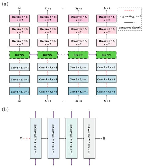
Figure 1.
(a) Network architecture of the convolutional neural networks (CNNs) combined with bi-directional convolutional long short-term memory networks (CNN-BiConvLSTM) model. (b) Network architecture of bi-directional recurrent neural network (BiRNN) in (a). X denotes input radar images, E denotes features encoded by the CNN encoder, O denotes features encoded by the BiRNN encoder, and s denotes strides of the convolution.
2.2. Baseline Models
2.2.1. Traditional Baseline Models
The linear model is a basic and simple model since it takes only the temporal evolution of radar echoes into account. It calculates the linear trend between 2 radar images for each pixel and then interpolates or extrapolates these pixels using the corresponding trends. The optical flow model was constructed based on the Dense Inverse Search (DIS) algorithm. The DIS algorithm is a global optical flow algorithm proposed by Kroeger et al. [47], which allows the explicit estimation of the velocity of each image pixel based on an analysis of 2 adjacent radar images. The DIS algorithm was selected as a benchmark because of its high accuracy in the extrapolation and interpolation of radar images [12]. The implementation of the optical flow model can be summarized as follows:
- Calculate velocity field using the global DIS optical flow algorithm [47] based on the radar images at times and .
- Use a backward constant-vector [48] to interpolate or extrapolate each pixel according to the velocity field.
- Obtain an irregular point cloud that consists of the original radar pixels. Then interpolate the intensity of these displaced pixels in the original radar grid. The inverse distance weighted interpolation technique is used in the interpolation.
Figure 2 demonstrates an example of interpolating 3 radar frames from 2 adjacent radar images. The features of Radar (t) were propagated according to the calculated velocity field to generate intermediate frames Radar (t + 1), Radar (t + 2), and Radar (t + 3). Apparently, the observed radar image Radar (t + 4) was only used in velocity field calculation, and the shape of the echoes was fully dependent on the first frame.
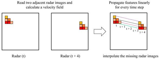
Figure 2.
Schematic diagram of interpolating three radar frames from two adjacent radar images using optical flow model.
2.2.2. Basic DNNs
The CNN-ConvLSTM model was constructed by replacing the BiconvLSTM module in the BiRNN encoder (Figure 1b) with the ConvLSTM module. The 3DCNN model was also constructed as an encoder–decoder structure, as shown in Figure 3. The encoder consisted of 3 3DCNNs (Conv3D), each followed by an average pooling (AvgPooling3D) layer. The decoder consisted of 3 3DCNN transpose (DeConv3D) layers, as shown in Figure 3. Unlike RNN-based models, the 3DCNN model extracted high-level features by using all radar images together. Meanwhile, all the output radar images were decoded from the high-level features. The leaky ReLU activity layer was used for all 3DCNN and 3DCNN transpose layers.
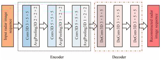
Figure 3.
Network architecture of the three-dimensional convolutional neural network (3DCNN) model.
3. Data and Experimental Design
3.1. Dataset
The radar dataset was constructed based on the radar reflectivity data of 11 S-band Doppler weather radar (Beijing Metstar Radar Co., Ltd., China) stations covering the Guangdong province from 2010 to 2019. The products of Constant Altitude Plan Position Indicator (CAPPI) [49] images with a resolution of 0.1 km were generated and used in the study. The dates of the radar data were chosen according to the rule that short-term heavy precipitation (greater than 20 mm/h) occurred at more than 3 automatic weather stations over Guangdong province. The size of the radar echo images was 256 × 256, and the limits of the values of radar reflectivity factors were 0 to 80 dBZ. To facilitate the study, the length of the sample sequences was extracted and fixed at 10. The training set and validation set were split by samples in 2010–2018 with sizes of 18,000 and 2000, respectively. The test set of size 2000 was retrieved from samples in 2019 to ensure independence.
3.2. Experimental Configuration
The CNN-BiConvLSTM model and basic DNNs were all optimized with Adam [50] by setting and , and the initial learning rate was set to 0.0005 with an exponential decay according to the formula:
where denotes the number of iterations. The loss function is a combination of losses according to the formula:
where denotes losses for all output radar images and denotes only missing positions of output radar images; denotes losses for values of reflectivity factors larger than 30 in all input radar images; and are chosen as the weights of losses. and are given more weight in order to emphasize the importance of missing frames and strong radar echoes. All the inputs were scaled by 80, and the outputs were limited to the range of 0 to 80. To simulate missing frames in real radar sequences, the input radar images were randomly masked before they were fed to the model during the training, following the rules below:
(1) Generate a random mask for a radar sequence of length 10. The number of masked radar images ranges from 0 to 10 with equal probability. All the masked images are set to zero.
(2) Randomly replace two positions of the mask by ones to ensure at least two real radar images in a sequence.
During inference, the input radar images were masked according to the real missing patterns. The scheme chart for the mask procedure and DNN model is shown in Figure 4. This procedure enabled the model to deal with any possible missing patterns. If no masks were given to the input radar images, the model would abstract features from every input radar image in the training procedure. However, in the inference model, the model will extract features from zero inputs as real radar images and subsequently obtain poor results. In the study, the missing pattern of a radar sequence of length 10 was denoted as 10 binary numbers, where element ‘0′ indicated missing frames and element ‘1′ indicated normal frames. The batch size was set to 8, and the training was stopped after ~160,000 iterations (i.e., 80 epochs). The mask ratio was gradually increased up to 100% at 10,000 iterations. The models were evaluated for every epoch, and the optimal model was chosen according to the highest validation loss for each model.
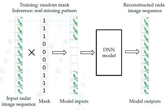
Figure 4.
Scheme chart for the masking procedure and the deep neuron network (DNN) model.
3.3. Evaluation Metrics
We evaluated the performances of all models with the mean absolute error (MAE), critical success index (CSI), and Heidke skill score (HSS) [51]. Mathematically, the CSI score was computed as
where hits correspond to true positives, misses correspond to false positives, and false alarms correspond to false negatives in the confusion matrix. The critical threshold was chosen to be 30 dBZ (CSI-30) or 40 dBZ (CSI-40). A higher CSI score denotes a better prediction with respect to a reflectivity factor larger than the threshold. The HSS score was computed as
where is the number of predictions (i.e., pixels in a predicted image), denotes forecasts categories, denotes the number of forecasts and observations both in category and and denote the total number of forecasts and observations in category , respectively. The predictions are classified into 5 classes according to the intervals (0, 20), (20, 30), (30, 40), (40, 50), and (50, 80). The HSS score reflects the accuracy of a prediction relative to that obtained by random chance. A higher HSS score denotes a better model.
4. Results
In this section, the CNN-BiConvLSTM model and baseline models were evaluated for the test datasets with comparative analysis. Section 4.1 evaluates the results for the case of interpolation, corresponding to several successive or discrete intermediate missing frames in a radar sequence. Because the extrapolation can also be used to reconstructing missing frames, Section 4.2 further evaluates and compares the results for the case of extrapolation to verify whether the effectiveness of a model was better for interpolated cases. The influences of the quality of input radar sequences and model sizes on the performance of the models are investigated in Section 4.3.
4.1. Evaluation Results for the Case of Interpolation
Six different missing patterns were involved in the evaluations in order to investigate the influence of the numbers of missing frames on the models. The first 5 patterns miss 1, 2, 4, 6, 8 successive intermediate frames, respectively. The last missing pattern misses 4 discrete intermediate frames. The chosen missing patterns were representative because the number of successive missing frames was usually not too high in real radar data sets. Table 1 presents the MAE, CSI-40 scores and HSS scores for the CNN-BiConvLSTM model and baseline models with respect to several specific missing patterns. It was found that the performances of the CNN-BiConvLSTM model were the best among all the models and for all evaluation metrics and missing patterns involved. Apart from the CNN-BiConvLSTM model, the 3DCNN model generally performed better than the other models. Whereas for the CNN-ConvLSTM, the performances were unstable and are highly dependent on evaluation metrics and missing patterns. Specifically, the MAE and HSS scores for the CNN-ConvLSTM model were generally better than those of the optical flow model, but the CSI-40 scores were poorer than those of the optical flow model, especially under conditions of multiple successive missing frames (e.g., ‘1000000001’). Considering identical network structures between CNN-BiConvLSTM and CNN-ConvLSTM except for the bidirectional structure, it can be inferred that the spatial–temporal information in both directions is quite important. This was also the reason why the 3DCNN model achieved a better performance. The output radar images in the 3DCNN model used encoded features from all input radar images (Figure 3), while the output radar images in the CNN-ConvLSTM model used only encoded features from previous radar images. When features from subsequent radar images were taken into account in the CNN-ConvLSTM model (i.e., CNN-BiConvLSTM), the performances were superior to those of the 3DCNN model. This result also implied the higher effectiveness of RNNs in extracting spatial–temporal features compared to CNNs. In addition to higher average scores, the scores of each sample for the CNN-BiConvLSTM model were found mostly higher than that of the baseline models. Figure 5 shows histograms for the missing pattern of ‘1110000111’ as a representative case. The differences of scores between the CNN-BiConvLSTM model and baseline models for test samples were found mostly less than zero for the MAE and larger than zero for the CSI scores and HSS scores. The results further highlighted the effectiveness of the CNN-BiConvLSTM model.

Table 1.
Evaluation results of mean absolute error (MAE), Critical success index (CSI)-40 scores, and Heidke skill score (HSS) scores for the bi-directional convolutional long short-term memory networks (CNN-BiConvLSTM) model and baseline models and for 6 missing patterns with respect to interpolation.
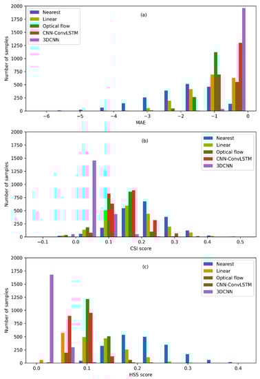
Figure 5.
Histograms for the differences of mean absolute error (MAE) (a), Critical success index (CSI)-40 scores (b), and Heidke skill score (HSS) scores (c) between the CNN-BiConvLSTM model and baseline models for the missing pattern of ‘1110000111’.
As the number of successive missing frames increased, the performance of all the models got worse. This was reasonable since the models received less information but generated many more outputs. Nonetheless, the CNN-BiConvLSTM model performed well enough when missing 4 successive frames, and even better than traditional interpolation models when only 1 frame was missing. For the case of 4 discrete intermediate frames missing (i.e., 1010101011), the performances of the linear model, the optical flow model, and CNN-BiConvLSTM were found to be nearly equivalent to those of 1 intermediate frame missing. This implied that the CNN-BiConvLSTM model did well in reconstructing discrete intermediate missing frames without losing accuracy, as the linear model and the optical flow model did. While the latter models used only 2 adjacent frames before and after missing frames to generate an interpolation, the CNN-BiConvLSTM model learned regularities from the whole radar sequence and may obtain higher accuracy. By contrast, the performances of the CNN-ConvLSTM model and the 3DCNN model in the case of 4 discrete intermediate frames missing were slightly unstable.
To provide more detail, Figure 6 shows an example of reconstructing missing radar images with the CNN-BiConvLSTM model for all 6 missing patterns. It was found that the reconstructed radar images were quite similar to the ground truth with respect to the shapes and values of the radar echoes. The most encouraging success was the good reproduction of newly emerging and moving radar echoes in the west of the radar images (red boxes in Figure 6). This can clearly be observed for the results of missing patterns ‘1100000011’ (the 5th line in Figure 6) and ‘1000000001’ (the 6th line in Figure 6). The details of the radar echoes were indeed less distinct as the number of missing frames increased, which agreed with the evaluation results.
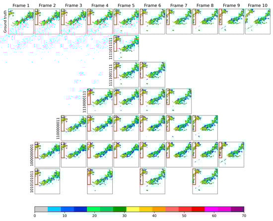
Figure 6.
Example of reconstructing missing radar frames with the CNN-BiConvLSTM model. The first line shows the input radar images (ground truths); the second line to the seventh line show reconstructed radar images for 6 specified missing patterns.
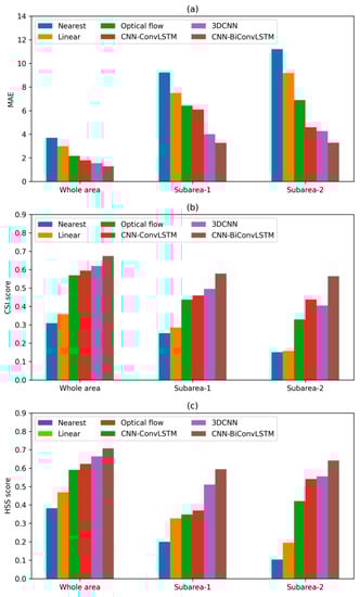
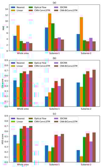
The reconstructed radar images for the selected example with respect to different models are shown in Figure 7, but only for the missing pattern ‘1110000111’. The performances of the CNN-BiConvLSTM model and the 3DCNN model were better on the whole, but with slightly more detailed echoes for the CNN-BiConvLSTM model. The reconstructed radar images from the CNN-ConvLSTM model lost much more detail compared to the ground truth. For the linear model, a large area of weak radar echo appeared around ground truth, and the strong radar echoes were diluted to some extent. For the optical flow model, the intensity of the radar echoes behaved quite well but exhibited an incorrect and fixed shape. More seriously, the reflectivity factors in some of the marginal areas in the reconstructed images were filled with zeros since the radar echoes moved out to other regions following the velocity field. Two subareas were selected to further demonstrate the effectiveness of different models for the marginal area (red and black boxes in Figure 7). The corresponding scores are shown in Figure 8. It was obvious that the traditional methods were quite unsuccessful in the two subareas, especially for subarea-2. The locations of the clear sky were quite distinct and correct for the reconstructed radar images in subarea-2 for the 3DCNN model and the CNN-BiConvLSTM model, but were not quite correct for the other models. In addition, the movements of radar echoes in subarea-1 can also be clearly observed for the 3DCNN model and the CNN-BiConvLSTM model but did not occur for the other models. In addition, the scores, which exclude the marginal area, were also tested, and they indeed showed slightly higher scores, but the order of the scores did not change. In summary, the CNN-BiConvLSTM model outperformed all the baseline models involved.
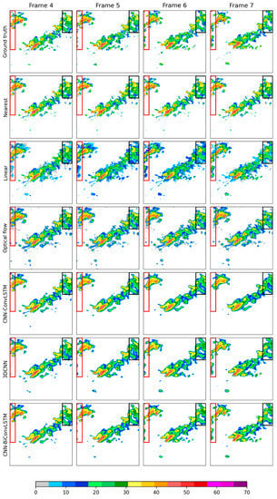
Figure 7.
Comparison of different models in reconstructing missing radar frames for the missing pattern of ‘1110000111’. The 1st line shows the fourth to the 7th input radar images (ground truths); the 2d to the 7th lines show the reconstructed radar images from different models.
4.2. Evaluation and Comparison for the Case of Extrapolation
Relative scores for models with respect to 5 missing patterns in the case of extrapolation were evaluated and presented in Table 2. To investigate the influence of the positions and number of missing frames on the models, the 5 specific missing patterns were chosen as follows: The first 4 patterns missed 1, 2, 3, and 4 successive radar images at the end of the sequence, respectively; The 5th pattern missed 3 successive radar images at the beginning of the sequence. Overall, the performances of the CNN-BiConvLSTM model were found to be the best in the case of interpolation, but were very close to those of the CNN-ConvLSTM model apart from missing pattern ‘0001111111’. This result suggested that the bidirectional architecture provided only a little improvement for the extrapolation compared to one direction. The good performance of the CNN-ConvLSTM model was consistent with previous studies in which the effectiveness of the ConvLSTM model was better than for optical flow methods [28]. The performances of 3DCNN were comparable to the optical flow model for the metrics of the MAE and HSS scores but were poorer for the CSI-40 scores. The linear model failed for all the missing patterns since the differences in pixel-wise reflectivity factors between two adjacent radar images were extremely unstable. The direction of extrapolation was found to have little effect on the performance of the models except for CNN-ConvLSTM when considering the scores for the missing pattern ‘0001111111’. In addition, the performances of all models become poorer as the number of missing frames increases in the case of interpolation.
Table 2.
Evaluation results of MAE, CSI-40 scores, and HSS scores for the CNN-BiConvLSTM model and baseline models, and for 5 missing patterns with respect to extrapolation.
Figure 9 shows an example of extrapolation with missing pattern ‘1111111000’ for all the models tested in this study. The failure of the linear model was quite obvious. The clear sky area in the western margin area (the fourth line in Figure 9) revealed the poor ability of the optical flow method in dealing with newly emerging radar echoes. The extrapolated radar images of the CNN-ConvLSTM model, the 3DCNN model, and the CNN-BiConvLSTM model showed features close to the ground truth, but more detailed radar echoes can be obtained by the CNN-ConvLSTM model and the CNN-BiConvLSTM model. All these features can be clearly observed in the red and black boxes in Figure 9. The corresponding scores are shown in Figure 10. For this example, apart from the nearest neighbor approach and linear interpolation, which showed poor results, the other methods showed comparable results for the whole area and for subarea-2. The optical method was quite unsuccessful for subarea-1 because of the movements of the radar echoes.
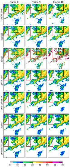
Figure 9.
Comparison of different models in reconstructing missing radar frames for the missing pattern ‘1111111000’. The first line shows the 7th and 10th input radar images (ground truths); the 2nd line to the 7th line show reconstructed radar images from different models.
On the whole, the effectiveness of the extrapolation was poorer than that in the interpolation experiments. To reconstruct 1 or 2 missing frames, extrapolation of 1 frame can be substituted. The evaluation results showed lower scores of the extrapolation models than the interpolation models. For instance, HSS scores of 0.7465 and 0.7305 for the case of interpolation by the CNN-BiConvLSTM model with missing patterns ‘1111011111’ and ‘1111001111’, and 0.7112 for the case of extrapolation with missing pattern ‘1111111110’, respectively. Similarly, to reconstruct 3–4, 5–6, and 7–8 missing frames, extrapolation of 2, 3, and 4 frames, respectively, can be substituted. For the case of reconstructing 5–6 missing frames, the performances of interpolation models were still better. While for the case of reconstructing 8 missing frames, the performances of interpolation and extrapolation models were comparable. This may imply the availability of both kinds of models when plenty of successive radar images are missing. However, this was not a solid conclusion since there were only two valid radar images in the input sequences. A better performance may be obtained when longer radar image sequences are used, and the effectiveness of interpolation models is probably still superior to that of extrapolation models for the case of multiple frames being missing.
4.3. Influence of Data Quality and Model Size
In addition to missing frames, the quality of radar images is another tough problem. The poor quality of radar images is mainly exhibited by the disappearance of part of the radar echo. This may originate from a quality control process or missing data at some radar station, which causes incomplete radar images when radar images are concatenated. Whether the quality of the radar echo sequences may influence the effectiveness of interpolation models is another important issue to be considered. We tested 1000 low-quality radar sequences for all interpolation models. Since the ground truth here is not a robust representation of the reasonable truth, the statistical evaluations were not quite suitable. Indeed, the performances of models on different low-quality radar sequences were quite consistent. Thus, several examples are presented to illustrate the influence of data quality as a representative case for the models involved.
Figure 11 shows an example of the influence of data quality for all interpolation models with missing pattern ‘1010101011’. Apparently, the 2nd, 4th, and 7th frames were less qualified images. For the linear model with missing pattern ‘1010101011’, the reconstructed frames 6 and 8 showed poor performances due to the large and unreasonable differences between input frames 5 and 7, and frames 7 and 9, respectively. For the optical model, reconstructed frame 8 showed poor performance. The poor result was caused mainly by the incorrect optical flow calculation of input frame 7 and frame 8. It is worth noting that reconstructed frame 6 was quite reasonable, although the adjacent frame 7 was a less qualified image and was used in the optical flow calculation. This is because the calculation of optical flow relies on the order of the image sequences. For three DNN interpolation models, all the reconstructed frames were surprisingly reasonable, although more details were shown for the CNN-BiConvLSTM model. For interpolation of frame 2 and frame 4 for all the models, it was found that the less qualified images can be well replaced by the reconstructed images, provided that the adjacent frames were well qualified. This was an encouraging result since it implies the potential of using interpolation methods to improve the quality of radar data by treating the less qualified frame as missing, especially with an effective interpolation model.
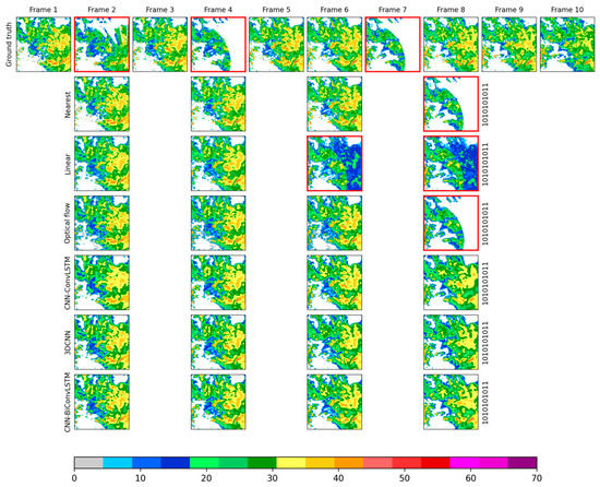
Figure 11.
Comparison of different models in reconstructing missing radar frames for the missing pattern ‘1010101011’. The first line shows the input radar images (ground truths); the 2nd to 7th lines show reconstructed radar images from different models.
Whether a DNN model, specifically the CNN-BiConvLSTM model, can deal with all the conditions with less qualified images was further investigated. By exploring plenty of samples, it was found that quite well-reconstructed frames can be obtained for the DNN models even with two less qualified adjacent frames. The only exception occurred when the less qualified images located at the ends of the sequence and the missing frames, were numerous enough. Figure 12 shows an example of the first frame being missing and interpolation by the CNN-BiConvLSTM model for missing patterns ‘1010101011’ and ‘1000000001’. The failure of the interpolation model was quite evident. Despite this failure, the problem can simply be avoided by extending the radar sequences by a step or two. Meanwhile, it was also found that the model performed well enough when the third frame was well qualified (third line in Figure 12).
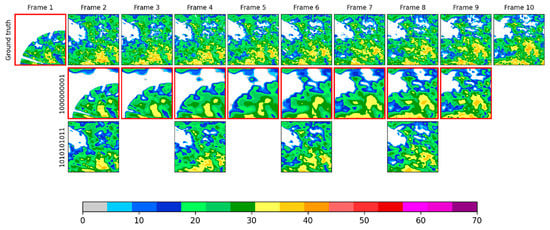
Figure 12.
Examples of reconstructing missing radar frames with the CNN-BiConvLSTM model for missing patterns ‘1000000001’ (second line) and ‘1010101011’ (third line). The first line shows the input radar images (ground truths).
In this study, the CNN-BiConvLSTM model was constructed as quite a small model with 2.3 million parameters in total. Larger models denoted CNN-BiConvLSTM-M with 3.3 million parameters in total, and CNN-BiConvLSTM-L with 10.3 million parameters in total were also constructed and evaluated. Table 3 presents the results. The performances of the CNN-BiConvLSTM model were found to have improved monotonously for all missing patterns as the size of the models increased, indicating that the spatial–temporal variations can be better simulated by models with more parameters and probably by more sophisticated RNN modules.
Table 3.
Evaluation results of MAE, CSI-40 scores, and HSS scores for the CNN-BiConvLSTM model with different model sizes and for 6 missing patterns with respect to interpolation.
5. Conclusions and Discussion
In this paper, we propose a DNN model, the CNN-BiConvLSTM model, to reconstruct missing data in weather radar image sequences. The model is able to deal with arbitrary missing patterns by using a proposed training scheme. To verify the effectiveness of the model, the nearest neighbor approach, linear interpolation, the optical flow method, and two DNN models, CNN-ConvLSTM and 3DCNN, were included in the study and were evaluated to perform a comparative analysis. The performances of the CNN-BiConvLSTM model were better than for all baseline models for the missing patterns and evaluation metrics involved. Two baseline DNN models, the CNN-ConvLSTM model, and the 3DCNN model generate reasonable radar images but lose much more detail. The weaknesses of traditional approaches are quite obvious: The nearest neighbor approach generates fixed radar echoes and obtains the lowest scores; the linear model generates lots of unreal weak radar echoes; the optical flow model generates radar echoes of quite fixed shape and zero values in the marginal area.
The DNN models, especially for the CNN-BiConvLSTM model, are quite robust to the quality of the input data sequences. The linear model and the optical flow model largely failed in less qualified input radar sequences. Furthermore, the performances of the CNN-BiConvLSTM mode were found to improve with the number of model parameters, indicating potential improvements to the model. In summary, the CNN-BiConvLSTM model shows a powerful ability in reconstructing missing observations in radar data sequences. The main reason is that the DNN models are able to learn intrinsic spatial–temporal features based on numerous radar image sequences, especially for the CNN-BiConvLSTM model, while the traditional methods are based on empirical assumptions, which is not quite appropriate, such as persistence (nearest neighbor approach), linear temporal evolution at each grid (linear interpolation), and linear motion of radar echoes (optical flow method).
To the best of our knowledge, no previous research has experimented with DNNs in reconstructing missing radar images. Most studies focus on predicting future radar images rather than improving radar data themselves [52]. Experimental results (Section 4.2) show that the effectiveness of the models for the interpolation cases is superior to that of extrapolation (i.e., prediction) cases in reconstructing radar images, indicating the significance of our study. The results also suggest that the input radar sequences should include valid first and last frames in the reconstruction process. Other relative studies focus mainly on interpolating satellite images using DNNs to improve temporal resolution [53,54]. However, the quantitative evaluations for these temporal super-resolution experiments are quite limited because not all interpolated frames have ground truths. Therefore, the accuracy of reconstructed radar images is expected to be higher. For these reasons, we implemented an RNN-based DNN model with encoder–decoder architecture as a benchmark in order to improve the quality of weather radar datasets. Based on the formulation of our work, more sophisticated RNN modules, such as PredRNN and MIM [40,41], can easily be applied to further improve the model performance. Slim architecture can also be used in the CNN encoder and CNN decoder to reduce computational complexity but without reducing accuracy [55].
In addition to missing radar images, we noticed that the less qualified radar images could also be reconstructed by the CNN-BiConvLSTM model as long as they are fed to the model as missing data (Figure 11). This result suggests the potential use of DNN models in weather radar data quality control. Although no relevant research has been reported, applications of image restoration in the field of computer vision may provide references [56,57]. It should be noted that the models and their evaluations are based on radar data sequences of length 10. Nonetheless, the results are largely representative since there are not usually longer lengths of successive missing frames in reality. Models that deal with much longer lengths of radar data sequences can be easily constructed by following this study. In addition, based on the improved weather radar datasets through reconstructing missing radar data, improvements in QPE and QPF products are to be expected and are worth investigating in the future.
Author Contributions
All authors contributed to this manuscript: Conceptualization, L.G.; methodology, L.G. and Y.Z.; software, L.G., Y.G., J.X., B.L., and Y.G.; experiment and analysis, L.G., and Y.Z.; data curation, X.C., and M.L.; writing—original draft preparation, L.G.; writing—review and editing, L.G., Y.Z., Y.W., J.X., X.C., B.L., M.L., and Y.G.; visualization, Y.Z. and L.G.; supervision, Y.W.; funding acquisition, Y.W., X.C., and M.L. All authors have read and agreed to the published version of the manuscript.
Funding
This work was supported in part by the Basic Creative Research Fund of Huafeng Meteorological Media Group (CY—J2020001), and in part by the National Key Research and Development Program of China for Intergovernmental Cooperation (2019YFE0110100), and in part by the Basic Research Fund of Chinese Academy of Meteorological Sciences (2020Z011).
Institutional Review Board Statement
Not applicable.
Informed Consent Statement
Not applicable.
Data Availability Statement
Restrictions apply to the availability of these data. Data was obtained from Shenzhen Meteorological Bureau and are available https://opendata.sz.gov.cn/data/dataSet/toDataSet/dept/9 (accessed on 22 February 2021) with the permission of Shenzhen Meteorological Bureau.
Acknowledgments
We thank Jin Ma (Institute for Marine and Atmospheric research Utrecht, Utrecht University, The Netherlands) for helpful discussions in this study. We also thank two anonymous reviewers for their constructive comments.
Conflicts of Interest
The authors declare no conflict of interest.
References
- Chandrasekar, V.; Wang, Y.; Chen, H. The CASA quantitative precipitation estimation system: A five year validation study. Nat. Hazards Earth Syst. Sci. 2012, 12, 2811–2820. [Google Scholar] [CrossRef]
- Huang, H.; Zhao, K.; Zhang, G.; Lin, Q.; Wen, L.; Chen, G.; Yang, Z.; Wang, M.; Hu, D. Quantitative Precipitation Estimation with Operational Polarimetric Radar Measurements in Southern China: A Differential Phase-Based Variational Approach. J. Atmos. Ocean. Technol. 2018, 35. [Google Scholar] [CrossRef]
- Liguori, S.; Rico-Ramirez, M. A review of current approaches to radar based Quantitative Precipitation Forecasts. Int. J. River Basin Manag. 2013, 12. [Google Scholar] [CrossRef]
- Novák, P.; Březková, L.; Frolík, P.; Šálek, M. Quantitative precipitation forecast using radar echo extrapolation. Atmos. Res. 2007, 93. [Google Scholar] [CrossRef]
- Lepot, M.; Aubin, J.-B.; Clemens, F.H.L.R. Interpolation in Time Series: An Introductive Overview of Existing Methods, Their Performance Criteria and Uncertainty Assessment. Water 2017, 9, 796. [Google Scholar] [CrossRef]
- Cosgrove, B.A.; Lohmann, D.; Mitchell, K.E.; Houser, P.R.; Wood, E.F.; Schaake, J.C.; Robock, A.; Marshall, C.; Sheffield, J.; Duan, Q.; et al. Real-time and retrospective forcing in the North American Land Data Assimilation System (NLDAS) project. J. Geophys. Res. Atmos. 2003, 108. [Google Scholar] [CrossRef]
- Piccolo, F.; Chirico, G.B. Sampling errors in rainfall measurements by weather radar. Adv. Geosci. 2005, 2. [Google Scholar] [CrossRef]
- Langston, C.; Zhang, J.; Howard, K. Four-Dimensional Dynamic Radar Mosaic. J. Atmos. Ocean. Technol. 2007, 24. [Google Scholar] [CrossRef]
- Ruzanski, E.; Chandrasekar, V. Weather Radar Data Interpolation Using a Kernel-Based Lagrangian Nowcasting Technique. IEEE Trans. Geosci. Remote Sens. 2015, 53, 3073–3083. [Google Scholar] [CrossRef]
- Sakaino, H. Spatio-Temporal Image Pattern Prediction Method Based on a Physical Model With Time-Varying Optical Flow. IEEE Trans. Geosci. Remote Sens. 2013, 51, 3023–3036. [Google Scholar] [CrossRef]
- Li, L.; Schmid, W.; Joss, J. Nowcasting of Motion and Growth of Precipitation with Radar over a Complex Orography. J. Appl. Meteorol. 1995, 34, 1286–1300. [Google Scholar] [CrossRef]
- Ayzel, G.; Heistermann, M.; Winterrath, T. Optical flow models as an open benchmark for radar-based precipitation nowcasting (rainymotion v0.1). Geosci. Model Dev. 2019, 12, 1387–1402. [Google Scholar] [CrossRef]
- Bentamy, A.; Fillon, D.C. Gridded surface wind fields from Metop/ASCAT measurements. Int. J. Remote Sens. 2012, 33, 1729–1754. [Google Scholar] [CrossRef]
- Paulson, K.S. Fractal interpolation of rain rate time series. J. Geophys. Res. 2004, 109. [Google Scholar] [CrossRef]
- Woo, W.-C.; Wong, W.-K. Operational application of optical flow techniques to radar-based rainfall nowcasting. Atmosphere 2017, 8, 48. [Google Scholar] [CrossRef]
- Germann, U.; Zawadzki, I. Scale-Dependence of the Predictability of Precipitation from Continental Radar Images. Part I: Description of the Methodology. Mon. Weather Rev. 2002, 130, 2859–2873. [Google Scholar] [CrossRef]
- Zahraei, A.; Hsu, K.-L.; Sorooshian, S.; Gourley, J.J.; Lakshmanan, V.; Hong, Y.; Bellerby, T. Quantitative Precipitation Nowcasting: A Lagrangian Pixel-Based Approach. Atmos. Res. 2012, 118, 418–434. [Google Scholar] [CrossRef]
- Liu, Y.; Xi, D.-G.; Li, Z.-L.; Hong, Y. A new methodology for pixel-quantitative precipitation nowcasting using a pyramid Lucas Kanade optical flow approach. J. Hydrol. 2015, 529, 354–364. [Google Scholar] [CrossRef]
- Grecu, M.; Krajewski, W.F. A large-sample investigation of statistical procedures for radar-based short-term quantitative precipitation forecasting. J. Hydrol. 2000, 239, 69–84. [Google Scholar] [CrossRef]
- Austin, G.L.; Bellon, A. The use of digital weather radar records for short-term precipitation forecasting. Q. J. R. Meteorol. Soc. 1974, 100, 658–664. [Google Scholar] [CrossRef]
- Lucas, B.D.; Kanade, T. An iterative image registration technique with an application to stereo vision. In Proceedings of the International Joint Conference on Artificial Intelligence, Vancouver, BC, Canada, 24–28 August 1981; pp. 674–679. [Google Scholar]
- Horn, B.K.P.; Schunck, B.G. Determining optical flow. Artif. Intell. 1981, 17, 185–203. [Google Scholar] [CrossRef]
- Joyce, R.; Janowiak, J.; Arkin, P.; Xie, P. CMORPH: A Method That Produces Global Precipitation Estimates from Passive Microwave and Infrared Data at High Spatial and Temporal Resolution. J. Hydrol. 2004, 5. [Google Scholar] [CrossRef]
- Ruzanski, E.; Chandrasekar, V.; Wang, Y. The CASA Nowcasting System. J. Atmos. Ocean. Technol. 2011, 28, 640–655. [Google Scholar] [CrossRef]
- Thorndahl, S.; Nielsen, J.E.; Rasmussen, M.R. Bias adjustment and advection interpolation of long-term high resolution radar rainfall series. J. Hydrol. 2014, 508, 214–226. [Google Scholar] [CrossRef]
- Nielsen, J.E.; Thorndahl, S.; Rasmussen, M.R. A numerical method to generate high temporal resolution precipitation time series by combining weather radar measurements with a nowcast model. Atmos. Res. 2014, 138, 1–12. [Google Scholar] [CrossRef]
- Ayzel, G.; Scheffer, T.; Heistermann, M. RainNet v1.0: A convolutional neural network for radar-based precipitation nowcasting. Geosci. Model Dev. 2020, 13, 2631–2644. [Google Scholar] [CrossRef]
- Shi, X.J.; Chen, Z.R.; Wang, H.; Yeung, D.Y.; Wong, W.K.; Woo, W.C. Convolutional LSTM network: A machine learning approach for precipitation nowcasting. In Proceedings of the 28th International Conference on Neural Information Processing Systems, Montreal, QC, Canada, 7–12 December 2015; pp. 802–810. [Google Scholar]
- Hu, Y.; Lu, X. Learning spatial-temporal features for video copy detection by the combination of CNN and RNN. J. Vis. Commun. Image Represent. 2018, 55, 21–29. [Google Scholar] [CrossRef]
- Zhang, T.; Zheng, W.; Cui, Z.; Zong, Y.; Li, Y. Spatial-Temporal Recurrent Neural Network for Emotion Recognition. IEEE Trans. Cybern. 2018, 839–847. [Google Scholar] [CrossRef] [PubMed]
- Fuentes-Pacheco, J.; Torres-Olivares, J.; Roman-Rangel, E.; Cervantes, S.; Juarez-Lopez, P.; Hermosillo-Valadez, J.; Rendón-Mancha, J.M. Fig Plant Segmentation from Aerial Images Using a Deep Convolutional Encoder-Decoder Network. Remote Sens. 2019, 11, 1157. [Google Scholar] [CrossRef]
- Javaloy, A.; García-Mateos, G. Text Normalization Using Encoder–Decoder Networks Based on the Causal Feature Extractor. Appl. Sci. 2020, 10, 4551. [Google Scholar] [CrossRef]
- Zhang, H.; Ma, C.; Pazzi, V.; Zou, Y.; Casagli, N. Microseismic Signal Denoising and Separation Based on Fully Convolutional Encoder–Decoder Network. Appl. Sci. 2020, 10, 6621. [Google Scholar] [CrossRef]
- Sutskever, I.; Vinyals, O.; Le, Q.V. Sequence to sequence learning with neural networks. In Advances in Neural Information Processing Systems; Neural Information Processing Systems Foundation, Inc.: South Lake Tahoe, NV, USA, 2014; pp. 3104–3112. [Google Scholar]
- Donahue, J.; Hendricks, L.; Guadarrama, S.; Rohrbach, M.; Venugopalan, S.; Darrell, T.; Saenko, K. Long-term recurrent convolutional networks for visual recognition and description. In Proceedings of the IEEE Conference on Computer Vision and Pattern Recognition, Boston, MA, USA, 7–12 June 2015; pp. 2625–2634. [Google Scholar]
- Hochreiter, S.; Schmidhuber, J. Long Short-term Memory. Neural Comput. 1997, 9, 1735–1780. [Google Scholar] [CrossRef]
- Srivastava, N.; Mansimov, E.; Salakhutdinov, R. Unsupervised learning of video representations using LSTMs. In Proceedings of the 32nd International Conference on International Conference on Machine Learning, Lille, France, 7–9 July 2015; Volume 37, pp. 843–852. [Google Scholar]
- Shi, X.; Gao, Z.; Lausen, L.; Wang, H.; Yeung, D.Y.; Wong, W.K.; Woo, W.C. Deep learning for precipitation nowcasting: A benchmark and a new model. In Proceedings of the 31st International Conference on Neural Information Processing Systems, Long Beach, CA, USA, 4–9 December 2017; pp. 5622–5632. [Google Scholar]
- Wang, Y.; Long, M.; Wang, J.; Gao, Z.; Yu, P.S. PredRNN++: Towards a resolution of the deep-in-time dilemma in spatiotemporal predictive learning. Proc. Mach. Learn. Res. 2018, 80, 5123–5132. [Google Scholar]
- Wang, Y.; Long, M.; Wang, J.; Gao, Z.; Yu, P.S. PredRNN: Recurrent Neural Networks for Predictive Learning using Spatiotemporal LSTMs. In Advances in Neural Information Processing Systems 30; Guyon, I., Luxburg, U.V., Bengio, S., Wallach, H., Fergus, R., Vishwanathan, S., Garnett, R., Eds.; Curran Associates, Inc.: New York, NY, USA, 2017; pp. 879–888. [Google Scholar]
- Wang, Y.; Zhang, J.; Zhu, H.; Long, M.; Wang, J.; Yu, P.S. Memory in memory: A predictive neural network for learning higher-order non-stationarity from spatiotemporal dynamics. In Proceedings of the IEEE Conference on Computer Vision and Pattern Recognition, Long Beach, CA, USA, 16–20 June 2019; pp. 9154–9162. [Google Scholar]
- Wang, Y.; Jiang, L.; Yang, M.H.; Li, L.J.; Long, M.; Fei-Fei, L. Eidetic 3D LSTM: A Model for Video Prediction and Beyond. In Proceedings of the International Conference on Learning Representations, New Orleans, LA, USA, 6–9 May 2019. [Google Scholar]
- Ronneberger, O.; Fischer, P.; Brox, T. U-Net: Convolutional Networks for Biomedical Image Segmentation. Exp. Algorithms 2015, 9351, 234–241. [Google Scholar]
- Peng, D.; Zhang, Y.; Guan, H. End-to-End Change Detection for High Resolution Satellite Images Using Improved UNet++. Remote Sens. 2019, 11, 1382. [Google Scholar] [CrossRef]
- Chen, S.; Zhang, S.; Geng, H.; Chen, Y.; Zhang, C.; Min, J. Strong Spatiotemporal Radar Echo Nowcasting Combining 3DCNN and Bi-Directional Convolutional LSTM. Atmosphere 2020, 11, 569. [Google Scholar] [CrossRef]
- Chang, Y.; Luo, B. Bidirectional Convolutional LSTM Neural Network for Remote Sensing Image Super-Resolution. Remote Sens. 2019, 11, 2333. [Google Scholar] [CrossRef]
- Kroeger, T.; Timofte, R.; Dai, D.; Van Gool, L. Fast optical flow using dense inverse search. In Proceedings of the European Conference on Computer Vision, Amsterdam, The Netherlands, 8–16 October 2016; pp. 471–488. [Google Scholar]
- Bowler, N.E.H.; Pierce, C.E.; Seed, A. Development of a precipitation nowcasting algorithm based upon optical flow techniques. J. Hydrol. 2004, 288, 74–91. [Google Scholar] [CrossRef]
- Mak Kwon, S.; Jung, S.-H.; Lee, G. Inter-comparison of radar rainfall rate using constant altitude plan position indicator and hybrid surface rainfall maps. J. Hydrol. 2015, 531, 234–247. [Google Scholar] [CrossRef]
- Kingma, D.; Ba, J. Adam: A method for Stochastic Optimization. In Proceedings of the 3rd International Conference for Learning Representations, San Diego, CA, USA, 7–9 May 2015. [Google Scholar]
- Woodcock, F. The Evaluation of Yes/No Forecasts for Scientific and Administrative Purposes. Mon. Weather Rev. 1976, 104, 1209–1214. [Google Scholar] [CrossRef]
- Reichstein, M.; Camps-Valls, G.; Stevens, B.; Jung, M.; Denzler, J.; Carvalhais, N.; Prabhat. Deep learning and process understanding for data-driven Earth system science. Nature 2019, 566, 195–204. [Google Scholar] [CrossRef] [PubMed]
- Vandal, T.; Nemani, R. Temporal Interpolation of Geostationary Satellite Imagery with Task Specific Optical Flow. In Proceedings of the 1st ACM SIGKDD Workshop on Deep Learning for Spatiotemporal Data, Applications, and Systems (DeepSpatial ’20), Virtual Conference, 24 August 2020. [Google Scholar]
- Cruz, L.F.; Saito, P.T.M.; Bugatti, P.H. DeepCloud: An Investigation of Geostationary Satellite Imagery Frame Interpolation for Improved Temporal Resolution. In Proceedings of the 19th International Conference on Artificial Intelligence and Soft Computing, Zakopane, Poland, 12–14 October 2020. [Google Scholar]
- Winoto, A.S.; Kristianus, M.; Premachandra, C. Small and slim deep convolutional neural network for mobile device. IEEE Access 2020, 8, 125210–125222. [Google Scholar] [CrossRef]
- Tai, Y.; Yang, J.; Liu, X.; Xu, C. MemNet: A Persistent Memory Network for Image Restoration. In Proceedings of the IEEE International Conference on Computer Vision, Venice, Italy, 22–29 October 2017; pp. 4549–4557. [Google Scholar]
- Guo, Z.; Sun, Y.; Jian, M.; Zhang, X. Deep Residual Network with Sparse Feedback for Image Restoration. Appl. Sci. 2018, 8, 2417. [Google Scholar] [CrossRef]
Publisher’s Note: MDPI stays neutral with regard to jurisdictional claims in published maps and institutional affiliations. |
© 2021 by the authors. Licensee MDPI, Basel, Switzerland. This article is an open access article distributed under the terms and conditions of the Creative Commons Attribution (CC BY) license (http://creativecommons.org/licenses/by/4.0/).