Abstract
With the popularity of online opinion expressing, automatic sentiment analysis of images has gained considerable attention. Most methods focus on effectively extracting the sentimental features of images, such as enhancing local features through saliency detection or instance segmentation tools. However, as a high-level abstraction, the sentiment is difficult to accurately capture with the visual element because of the “affective gap”. Previous works have overlooked the contribution of the interaction among objects to the image sentiment. We aim to utilize interactive characteristics of objects in the sentimental space, inspired by human sentimental principles that each object contributes to the sentiment. To achieve this goal, we propose a framework to leverage the sentimental interaction characteristic based on a Graph Convolutional Network (GCN). We first utilize an off-the-shelf tool to recognize objects and build a graph over them. Visual features represent nodes, and the emotional distances between objects act as edges. Then, we employ GCNs to obtain the interaction features among objects, which are fused with the CNN output of the whole image to predict the final results. Experimental results show that our method exceeds the state-of-the-art algorithm. Demonstrating that the rational use of interaction features can improve performance for sentiment analysis.
1. Introduction
With the vast popularity of social networks, people tend to express their emotions and share their experiences online through posting images [1], which promotes the study of the principles of human emotion and the analysis and estimation of human behavior. Recently, with the wide application of convolution neural networks (CNNs) in emotion prediction, numerous studies [2,3,4] have proved the excellent ability of CNN to recognize the emotional features of images.
Based on the theory that the emotional cognition of a stimulus attracts more human attention [5], some researchers enriched emotional prediction with saliency detection or instance segmentation to extract more concrete emotional features [6,7,8]. Yang et al. [9] put forward the “Affective Regions” which are objects that convey significant sentiments, and proposed three fusion strategies for image features from the original image and “Affective Regions”. Alternatively, Wu et al. [8] utilized saliency detection to enhance the local features, improving the classification performance to a large margin.
“Affective Regions” or Local features in images play a crucial role in image emotion, and the above methods can effectively improve classification accuracy. However, although these methods have achieved great success, there are still some drawbacks. They focused on improving visual representations and ignored emotional effectiveness of objects, which leads to a non-tendential feature enhancement. For example, in an image expressing a positive sentiment, positivity is generated by interaction among objects. Separating objects and directly merging the features will lose much of the critical information of image.
Besides, they also introduce a certain degree of noise, which leads to the limited performance improvement obtained through visual feature enhancement. For example, in human common sense, “cat” tends to be a positive categorical word. As shown in Figure 1a,b, when “cat” forms the image with other neutral or positive objects, the image tends to be more positive, consistent with the conclusion that local features can improve accuracy. In the real world, however, there are complex images, as shown in Figure 1c,d, “cat” can be combined with other objects to express opposite emotional polarity, reflecting the effect of objects on emotional interactions. Specifically, in Figure 1d, the negative sentiment is not directly generated by the “cat” and “injector”, but the result of the interaction between the two in the emotional space. Indiscriminate feature fusion of such images will affect the performance of the classifier.
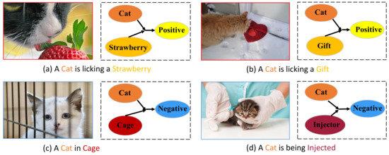
Figure 1.
Examples from EmotionROI dataset and social media: We use a graph model to describe the sentimental interaction between objects and the double arrow means the interaction in the process of human emotion reflection.
To address the abovementioned problems, we design a framework with two branches, one of which uses a deep network to extract visual emotional features in images. The other branch uses GCN to extract emotional interaction features of objects. Specially, we utilize Detectron2 to obtain the object category, location, and additional information in images. And then, SentiWordNet [10] is selected as an emotional dictionary to mark each category word with emotional intensity value. Based on the above information, we use the sentimental value of objects and visual characteristics in each image to build the corresponding graph model. Finally, we employ GCN to update and transmit node features, generate features after object interaction, which, together with visual components, serve as the basis for sentiment classification.
The contributions of this paper can be summarized as follows:
- We propose an end-to-end image sentiment analysis framework that employs GCN to extract sentimental interaction characteristics among objects. The proposed model makes extensive use of the interaction between objects in the emotional space rather than directly integrating the visual features.
- We design a method to construct graphs over images by utilizing Detectron2 and SentiWordNet. Based on the public datasets analysis, we leverage brightness and texture as the features of nodes and the distances in emotional space as edges, which can effectively describe the appearance characteristics of objects.
- We evaluate our method on five affective datasets, and our method outperforms previous high-performing approaches.
We make all programs of our model publicly available for research purposes https://github.com/Vander111/Sentimental-Interaction-Network.
2. Related Work
2.1. Visual Sentiment Prediction
Existing methods can be classified into two groups: dimensional spaces and categorical states. Dimensional spaces methods employ valence-arousal space [11] or activity-weight-heat space [12] to represent emotions. On the contrary, categorical states methods classify emotions into corresponding categories [13,14], which is easier for people to understand, and our work falls into categorical states group.
Feature extraction is of vital importance to emotion analysis, various kinds of features may contribute to the emotion of images [15]. Some researchers have been devoting themselves to exploring emotional features and bridging the “affective gap”, which can be defined as the lack of coincidence between image features and user emotional response to the image [16]. Inspired by art and psychology, Machajdik and Hanbury [14] designed low-level features such as color, texture, and composition. Zhao et al. [17] proposed extensive use of visual image information, social context related to the corresponding users, the temporal evolution of emotion, and the location information of images to predict personalized emotions of a specified social media user.
With the availability of large-scale image datasets such as ImageNet and the wide application of deep learning, the ability of convolutional neural networks to learn discriminative features has been recognized. You et al. [3] fine-tuned the pre-trained AlexNet on ImageNet to classify emotions into eight categories. Yang et al. [18] integrated deep metric learning with sentiment classification and proposed a multi-task framework for affective image classification and retrieval.
Sun et al. [19] discovered affective regions based on an object proposal algorithm and extracted corresponding in-depth features for classification. Later, You et al. [20] adopted an attention algorithm to utilize localized visual features and got better emotional classification performance than using global visual features. To mine emotional features in images more accurately, Zheng et al. [6] combined the saliency detection method with image sentiment analysis. They concluded that images containing prominent artificial objects or faces, or indoor and low depth of field images, often express emotions through their saliency regions. To enhance the work theme, photographers blurred the background to emphasize the main body of the picture [14], which led to the birth of close-up or low-depth photographs. Therefore, the focus area in low-depth images fully expresses the information that the photographer and forwarder want to tell, especially emotional information.
On the other hand, when natural objects are more prominent than artificial objects or do not contain faces, or open-field images, emotional information is usually not transmitted only through their saliency areas. Based on these studies, Fan et al. [7] established an image dataset labeled with statistical data of eye-trackers on human attention to exploring the relationship between human attention mechanisms and emotional characteristics. Yang et al. [9] synthetically considered image objects and emotional factors and obtained better sentiment analysis results by combining the two pieces of information.
Such methods make efforts in extracting emotional features accurately to improve classification accuracy. However, as an integral part of an image, objects may carry emotional information. Ignoring the interaction between objects is unreliable and insufficient. This paper selects the graph model and graph convolution network to generate sentimental interaction information and realize the sentiment analysis task.
2.2. Graph Convolutional Network(GCN)
The notion of graph neural networks was first outlined in Gori et al. [21] and further expound in Scarselli et al. [22]. However, these initial methods required costly neural “message-passing” algorithms to convergence, which was prohibitively expensive on massive data. More recently, there have been many methods based on the notion of GCN, which originated from the graph convolutions based on the spectral graph theory of Bruna et al. [23]. Based on this work, a significant number of jobs were published and attracted the attention of researchers.
Compared with the deep learning model introduced above, the graph model virtually constructs relational models. Chen et al. [24] combined GCN with multi-label image recognition to learn inter-dependent object information from labels. A novel re-weighted strategy was designed to construct the correlation matrix for GCN, and they got a higher accuracy compared with many previous works. However, this method is based on the labeled objects information from the dataset, which needs many human resources.
In this paper, we employ the graph structure to capture and explore the object sentimental correlation dependency. Specifically, based on the graph, we utilize GCN to propagate sentimental information between objects and generate corresponding interaction features, which is further applied to the global image representation for the final image sentiment prediction. Simultaneously, we also designed a method to build graph models from images based on existing image emotion datasets and describe the relationship features of objects in the emotional space, which can save a lot of workforce annotation.
3. Method
3.1. Framework
This section aims to develop an algorithm to extract interaction feature without manual annotation and combine it with holistic representation for image sentiment analysis. As shown in Figure 2, given an image with sentiment label, we employ a panoptic segmentation model, i.e., Detectron2, to obtain category information of objects and based on which we build a graph to represent the relationships among objects. Then, we utilize the GCN to leverage the interaction feature of objects in the emotional space. Finally, the interactive features of objects are concatenated with the holistic representation (CNN branch) to generate the final predictions. In the application scenario, given an image, we first use the panoramic segmentation model for data preprocessing to obtain the object categories and location information and establish the graph model. The graph model and the image are input into the corresponding branch to get the final sentiment prediction result.
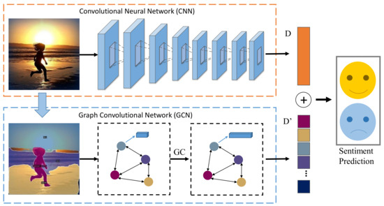
Figure 2.
Pipline of proposed approach framework.
3.2. Graph Construction
3.2.1. Objects Recognition
Sentiment is a complex logical response, to which the relations among objects in the image have a vital contribution. To deeply comprehend the interaction, we build a graph structure (relations among objects) to realize interaction features. And we take the categories of objects as the node and the hand-crafted feature as the representation of the object. However, existing image sentiment datasets, such as Flickr and Instagram (FI) [3], EmotionROI [25], etc., do not contain the object annotations. Inspired by the previous work [9], we employ the panoptic segmentation algorithm to detect objects.
We choose the R101-FPN model of Detectron2, containing 131 common object categories, such as “person”, “cat”,“bird”, “tree” etc., to realize recognition automatically. As shown in Figure 3, through the panoptic segmentation model, we process the original image Figure 3a to obtain the image Figure 3b containing the object category and location information.
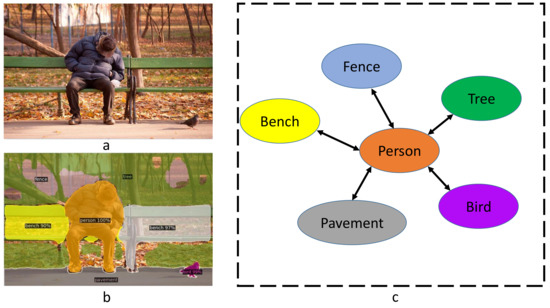
Figure 3.
Example of building graph model. Given the input image (a), Detectron2 can detect the region and categories of objects and (b) is the segmentation result. Based on the detection information, we build a graph (c) over the corresponding image.
3.2.2. Graph Representation
As a critical part of the graph structure, edges determine the weights of node information propagation and aggregation. In other fields, some researchers regard semantic relationship or co-occurrence frequency of objects as edges [1,26]. However, as a basic feature, there is still a gap between object semantics and sentiment, making it hard to accurately describe the sentimental relationship. Further, it is challenging to label abstract sentiments non-artificially due to the “affective gap” between low-level visual features and high-level sentiment. To solve this problem, we use the semantic relationship of objects in emotional space as the edges of the graph structure. Given the object category, we employ SentiWordNet as a sentiment annotation to label each category with sentimental information. SentiWordNet is a lexical resource for opinion mining that annotates the positive and negative values in the range [0,1] to words.
As shown in Equations (1) and (2), we retrieve words related to the object category in SentiWordNet, and judge the sentimental strength of the current word W with the average value of related words W, where W is the positive emotional strength, W is the negative emotion strength.
In particular, we stipulate that sentimental polarity of a word is determined by positive and negative strength. As shown in Equation (3), sentiment value S is the difference between the two sentimental intensity of words. In this way, positive words have a positive sentiment value, and negative words are the opposite. And S is in [−1, 1] because of the intensity of sentiments is between 0–1 in SentiWordNet.
Based on this, we design the method described in Equation (4). We can use a sentimental tendency of objects to measure the sentimental distance L between words W and W. When two words have the same sentimental tendency, we define the difference between the two sentiment values S and S as the distance in the sentimental space. On the contrary, we specify that two words with opposite emotional tendencies are added by one to enhance the sentimental difference. Further, we build the graph over the sentimental values and the object information. In Figure 3c, we show the relationship among node “person” and adjacent nodes, and the length of the edge reflects the distance between nodes.
3.2.3. Feature Representation
The graph structure describes the relationship between objects. And the nodes of the graph aim to describe the features of each object, where we select hand-crafted feature, intensity distribution, and texture feature as the representation of objects. Inspired by Machajdik [14], we calculate and analyze the image intensity characteristics on image datasets EmotionROI and FI. In detail, we quantify the intensity of each pixel to 0–10 and make histograms of intensity distribution. As shown in Figure 4, we find that the intensity of positive emotions (joy, surprise, etc.) is higher than that of negative emotions (anger, sadness, etc.) when the brightness is 4–6, while the intensity of negative emotions is higher on 1–2.
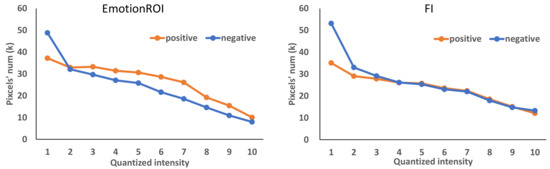
Figure 4.
The distribution curve of the number of brightness pixels of different emotion categories in the EmotionROI and Flickr and Instagram (FI) dataset.
The result shows that the intensity distribution can distinguish the sentimental polarity of the images to some extent. At the same time, we use the Gray Level Co-occurrence Matrix(GLCM) to describe the texture feature of each object in the image as a supplement to the image detail feature. Specifically, we quantified the luminance values as 0–255 and calculated a 256-dimensional eigenvector with 45 degrees as the parameter of GLCM. The node feature in the final graph model is a 512-dimensional eigenvector.
3.3. Interaction Graph Inference
Sentiment contains implicit relationships among the objects. Graph structure expresses low-level visual features and the relationship among objects, which is the source of interaction features, and inference is the process of generating interaction features. To simulate the interaction process, we employ GCN to propagate and aggregate the low-level features of objects under the supervision of sentimental distances. We select the stacked GCNs, in which the input of each layer is the output from the previous layer, and generate the new node feature .
The feature update process of the layer l is shown in Equation (5), is obtained by adding the edges of the graph model, namely the adjacency matrix and the identity matrix. is the output feature of the previous layer, is the output feature of the current layer, is the weight matrix of the current layer, and is the nonlinear activation function. is the degree matrix of , which is obtained by Equation (6).The first layer’s input is the initial node feature of 512 dimensions generated from the brightness histogram and GLCM introduced above. Also, the final output of the model is the feature vector of 2048 dimensions.
3.4. Visual Feature Representation
As a branch of machine learning, deep learning has been widely used in many fields, including sentiment image classification. Previous studies have proved that CNN network can effectively extract visual features in images, such as appearance and position, and map them to emotional space. In this work, we utilize CNN to realize the expression of visual image features. To make a fair comparison with previous works, we select the popularly used model VGGNet [27] as the backbone to verify the effectiveness of our method. For VGGNet, we adopt a fine-tuning strategy based on a pre-trained model on ImageNet and change the output number of the last fully connected layer from 4096 to 2048.
3.5. Gcn Based Classifier Learning
In the training process, we adopt the widely used concatenation method for feature fusion. In the visual feature branch, we change the last fully connected layer output of the VGG model to 2048 to describe the visual features extracted by the deep learning model. For the other branch, we process the graph model features in an average operation. In detail, the Equation (7) is used to calculate interaction feature , where n is the number of nodes in a graph model, is the feature of each node after graph convolution.
After the above processing, we employ the fusion method described in Equation (8) to calculate the fusion feature of visual and relationship, which is fed into the fully connected layer and realize the mapping between features and sentimental polarity. And the traditional cross entropy function is taken as the loss function, as shown in Equation (9), N is the number of training images, is the labels of images, and is the probability of prediction that 1 represents a positive sentiment and 0 means negative.
Specifically, is defined as Equation (10), where c is the number of classes. In this work, c is defined as 2, and is the output of the last fully connected layer.
4. Experiment Results
4.1. Datasets
We evaluate our framework on five public datasets: FI, Flickr [28], EmotionROI [25], Twitter I [29], Twitter II [28]. Figure 5 shows examples of these datasets. FI dataset is collected by querying with eight emotion categories (i.e., amusement, anger, awe, contentment, disgust, excitement, fear, sadness) as keywords from Flickr and Instagram, and ultimately gets 90,000 noisy images. The original dataset is further labeled by 225 Amazon Mechanical Turk (AMT) workers and resulted in 23,308 images receiving at least three agreements. The number of images in each emotion category is larger than 1000. Flickr contains 484,258 images in total, and the corresponding ANP automatically labeled each image. EmotionROI consists of 1980 images with six sentiment categories assembled from Flickr and annotated with 15 regions that evoke sentiments. Twitter I and Twitter II datasets are collected from social websites and labeled with two categories (i.e., positive and negative) by AMT workers, consisting of 1296 and 603 images. Specifically, we conducted training and testing on the three subsets of Twitter I: “Five agree”, “At least four agree” and “At least three agree”, which are filtered according to the annotation. For example, “Five agree” indicates that all the Five AMT workers rotate the same sentiment label for a given image. As shown in Table 1.
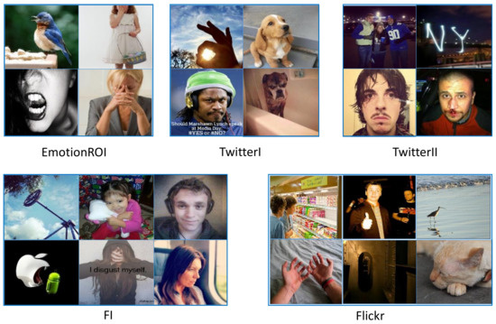
Figure 5.
Some examples in the five datasets.

Table 1.
Released and freely available datasets, where #Annotators respectively represent the number of annotators.
According to the affective model, the multi-label datasets EmotionROI and FI are divided into two parts: positive and negative, to achieve the sentimental polarity classification. EmotionROI has six emotion categories: anger, disgust, fear, joy, sadness, and surprise. Images with labels of anger, disgust, fear, sadness are relabeled as negative, and those with joy and surprise are labeled as positive. In the FI dataset, we divided Mikel’s eight emotion categories into binary labels based on [30], suggesting that amusement, contentment, excitement, and awe are mapped to the positive category, and sadness, anger, fear, and disgust are labeled as negative.
4.2. Implementation Details
Following previous works [9], we select VGGNet with 16 layers [25] as the backbone of the visual feature extraction and initialize it with the weights pre-trained on ImageNet. At the same time, we remove the last fully connected layer of the VGGNet. We randomly crop and resize the input images into 224 × 224 with random horizontal flip for data enhancement during the training. On FI, we select SGD as the optimizer and set Momentum to 0.9. The initial learning rate is 0.01, which drops by a factor of 10 per 20 epoch. And Table 2 shows the specific training strategy on the five datasets. In the relational feature branch, we use two GCN layers whose output dimensions are 1024 and 2048. 512-dimension vector characterizes each input node feature in the graph model. We adopted the same split and test method for the data set without specific division as Yang et al. [9]. For small-scale data sets, we refer to the strategy of Yang et al. [9], take the model parameters trained on the FI as initial weights, and fine-tune the model on the training set.
Table 2.
Setting of training parameters on the dataset of FI, Flickr, EmotionROI, Twitter I, Twitter II.
4.3. Evaluation Settings
To demonstrate the validity of our proposed framework for sentiment analysis, we evaluate the framework against several baseline methods, including methods using traditional features, CNN-based methods, and CNN-based methods combined with instance segmentation.
- The global color histograms (GCH) consists of 64-bin RGB histogram, and the local color histogram features (LCH) divide the image into 16 blocks and generate a 64-bin RGB histogram for each block [31].
- Borth et al. [28] propose SentiBank to describe the sentiment concept by 1200 adjectives noun pairs (ANPs), witch performs better for images with rich semantics.
- DeepSentibank [32] utilizes CNNs to discover ANPs and realizes visual sentiment concept classification. We apply the pre-trained DeepSentiBank to extract the 2089-dimension features from the last fully connected layer and employ LIBSVM for classification.
- You et al. [29] propose to select a potentially cleaner training dataset and design the PCNN, which is a progressive model based on CNNs.
- Yang et al. [9] employ object detection technique to produce the “Affective Regions” and propose three fusion strategy to generate the final predictions.
- Wu et al. [8] utilize saliency detection to enhance the local features, improving the classification performance to a large margin. And they adopt an ensemble strategy, which may contribute to performance improvement.
4.4. Classification Performance
We evaluate the classification performance on five affective datasets. Table 3 shows that the result of depth feature is higher than that of the hand-crafted feature and CNNs outperform the traditional methods. The VGGNet achieves significant performance improvements over the traditional methods such as DeepSentibank and PCNN on FI datasets of good quality and size. Simultaneously, due to the weak in annotation reliability, VGGNet does not make such significant progress on the Flickr dataset, indicating the dependence of the depth model on high-quality data annotation. Furthermore, our proposed method performs well compared with single model methods. For example, we achieve about 1.7% improvement on FI and 2.4% on EmotionROI dataset, which means that the sentimental interaction features extracted by us can effectively complete the image sentiment classification task. Besides, we adopt a simple ensemble strategy and achieve a better performance than state-of-the-art method.
Table 3.
Sentiment classification accuracy on FI, Flickr, Twitter I, Twitter II, EmotionROI. Results with bold indicate the best results compared with other algorithms.
4.5. The Role of Gcn Branch
As shown in Table 4, compared with the fine-tuned VGGNet, our method has an average performance improvement of 4.2%, which suggests the effectiveness of sentimental interaction characteristics in image emotion classification task.
Table 4.
The model performance comparison across image datasets. Results with bold indicate the best results compared with other algorithms.
4.6. Effect of Panoptic Segmentation
As a critical step in graph model construction, information of objects obtained through Detectron2 dramatically impacts the final performance. However, due to the lack of annotation with emotions and object categories, we adopt the panoptic segmentation model pre-trained on the COCO dataset, which contains a wide range of object categories. This situation leads to specific noise existing in the image information. As shown in Figure 6, the lefts are the original images from EmotionROI, and the detection results are on the right. In detail, there are omission cases (Figure 6d) and misclassification (Figure 6f) in detection results, which to a certain extent, affect the performance of the model, in the end, believe that if we can overcome this gap, our proposed method can obtain a better effect.
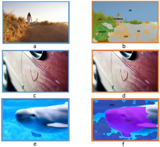
Figure 6.
Example of panoptic segmentation. Given the raw images (a,c,e), panoptic segmentation generates the accurate result (b), category missing result (d) and misclassification result (f).
As stated above, some object information of images cannot be extracted by the panoptic segmentation model. So we further analyze the result on emotionROI, of which each image is annotated with emotion and attractive regions manually by 15 persons and forms with the Emotion Stimuli Map. By comparing them with the Emotion Stimuli Map, our method fails to detect the critical objects in 77 images of a total of 590 testing images, as shown in Figure 7 mainly caused by the inconsistent categories of the panoptic segmentation model. A part of the EmotionROI images and the corresponding stimuli map is shown in Figure 7a,b, these images in the process of classification using only a part or even no object interaction information, but our method still predicts their categories correctly, indicating that visual features still play an essential role in the classification, and the interaction feature generated by GCN branch further improve the accuracy of the model.
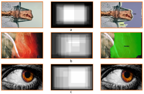
Figure 7.
Some example images and corresponding Emotion Stimuli Maps whose object information is broken extracted by panoptic segmentation model, but correctly predicted by our method. The lefts of (a–c) are the raw images, the middles are the corresponding stimuli map and the rights are the visual results of segmentation.
5. Conclusions
This paper addresses the problem of visual sentiment analysis based on graph convolutional networks and convolutional neural networks. Inspired by the principles of human emotion and observation, we find that each type of interaction among objects in the image has an essential impact on sentiment. We present a framework that consists of two branches for sentimental interaction representations learning. First of all, we design an algorithm to build a graph model on popular affective datasets without category information annotated based on panoptic segmentation information. As an essential part of the graph model, we define the objects in the images as nodes and calculate the edges between nodes in the graph model according to sentimental value of each objects. According to the effect of brightness on sentiment, we select brightness and texture features as node features. A stacked GCN model is used to generate the relational features describing the interaction results of objects and integrate them with the visual features extracted by VGGNet to realize the classification of image sentiment. Experimental results show the effectiveness of our method on five popular datasets. Furthermore, making more effective utilizing of objects interaction information remains a challenging problem.
Author Contributions
Conceptualization, H.Z. and S.D.; methodology, H.Z.; software, H.Z. and S.D.; validation, S.D.; formal analysis, H.Z. and S.D.; investigation, H.Z. and S.D.; resources, H.Z. and X.L.; data curation, X.L. and S.D.; writing—original draft preparation, H.Z. and S.D.; writing—review and editing, L.W. and G.S.; visualization, H.Z.; supervision, L.W. All authors have read and agreed to the published version of the manuscript.
Funding
This work was supported by National Natural Science Foundation of China grant numbers 61802011, 61702022.
Institutional Review Board Statement
Not applicable.
Informed Consent Statement
Not applicable.
Data Availability Statement
Data sharing is not applicable to this paper as no new data were created or analyzed in this study.
Conflicts of Interest
The authors declare no conflict of interest.
References
- Zhao, S.; Gao, Y.; Ding, G.; Chua, T. Real-time Multimedia Social Event Detection in Microblog. IEEE Trans. Cybern. 2017, 48, 3218–3231. [Google Scholar] [CrossRef]
- Peng, K.C.; Chen, T.; Sadovnik, A.; Gallagher, A.C. A Mixed Bag of Emotions: Model, Predict, and Transfer Emotion Distributions. In Proceedings of the IEEE Conference on Computer Vision and Pattern Recognition, Boston, MA, USA, 7–12 June 2015; pp. 860–868. [Google Scholar]
- You, Q.; Luo, J.; Jin, H.; Yang, J. Building A Large Scale Dataset for Image Emotion Recognition: The Fine Print and the Benchmark. In Proceedings of the Thirtieth AAAI Conference on Artificial Intelligence, Phoenix, AZ, USA, 12–17 February 2016; pp. 308–314. [Google Scholar]
- Zhu, X.; Li, L.; Zhang, W.; Rao, T.; Xu, M.; Huang, Q.; Xu, D. Dependency Exploitation: A Unified CNN-RNN Approach for Visual Emotion Recognition. In Proceedings of the 26th International Joint Conference on Artificial Intelligence, Melbourne, Australia, 19–25 August 2017; pp. 3595–3601. [Google Scholar]
- Compton, R.J. The Interface Between Emotion and Attention: A Review of Evidence from Psychology and Neuroscience. Behav. Cogn. Neurosci. Rev. 2003, 2, 115–129. [Google Scholar] [CrossRef]
- Zheng, H.; Chen, T.; You, Q.; Luo, J. When Saliency Meets Sentiment: Understanding How Image Content Invokes Emotion and Sentiment. In Proceedings of the 2017 IEEE International Conference on Image Processing, Beijing, China, 17–20 September 2017; pp. 630–634. [Google Scholar]
- Fan, S.; Shen, Z.; Jiang, M.; Koenig, B.L.; Xu, J.; Kankanhalli, M.S.; Zhao, Q. Emotional Attention: A Study of Image Sentiment and Visual Attention. In Proceedings of the IEEE Conference on Computer Vision and Pattern Recognition, Salt Lake City, UT, USA, 18–22 June 2018; pp. 7521–7531. [Google Scholar]
- Wu, L.; Qi, M.; Jian, M.; Zhang, H. Visual Sentiment Analysis by Combining Global and Local Information. Neural Process. Lett. 2019, 51, 1–13. [Google Scholar] [CrossRef]
- Yang, J.; She, D.; Sun, M.; Cheng, M.M.; Rosin, P.L.; Wang, L. Visual Sentiment Prediction Based on Automatic Discovery of Affective Regions. IEEE Trans. Multimed. 2018, 20, 2513–2525. [Google Scholar] [CrossRef]
- Esuli, A.; Sebastiani, F. Sentiwordnet: A Publicly Available Lexical Resource for Opinion Mining. In Proceedings of the Fifth International Conference on Language Resources and Evaluation, Genoa, Italy, 22–28 May 2006; pp. 417–422. [Google Scholar]
- Nicolaou, M.A.; Gunes, H.; Pantic, M. A Multi-layer Hybrid Framework for Dimensional Emotion Classification. In Proceedings of the 19th International Conference on Multimedia, Scottsdale, AZ, USA, 28 November–1 December 2011; pp. 933–936. [Google Scholar]
- Xu, M.; Jin, J.S.; Luo, S.; Duan, L. Hierarchical Movie Affective Content Analysis Based on Arousal and Valence Features. In Proceedings of the 16th International Conference on Multimedia, Vancouver, BC, Canada, 26–31 October 2008; pp. 677–680. [Google Scholar]
- Zhao, S.; Gao, Y.; Jiang, X.; Yao, H.; Chua, T.S.; Sun, X. Exploring Principles-of-art Features for Image Emotion Recognition. In Proceedings of the 22nd International Conference on Multimedia, Orlando, FL, USA, 3–7 November 2014; pp. 47–56. [Google Scholar]
- Machajdik, J.; Hanbury, A. Affective Image Classification Using Features Inspired by Psychology and Art Theory. In Proceedings of the 18th ACM international conference on Multimedia, Firenze, Italy, 25–29 October 2010; pp. 83–92. [Google Scholar]
- Zhao, S.; Yao, H.; Yang, Y.; Zhang, Y. Affective Image Retrieval via Multi-graph Learning. In Proceedings of the 22nd International Conference on Multimedia, Orlando, FL, USA, 3–7 November 2014; pp. 1025–1028. [Google Scholar]
- Hanjalic, A. Extracting Moods from Pictures and Sounds: Towards Truly Personalized TV. IEEE Signal Process. Mag. 2006, 23, 90–100. [Google Scholar] [CrossRef]
- Zhao, S.; Yao, H.; Gao, Y.; Ding, G.; Chua, T.S. Predicting Personalized Image Emotion Perceptions in Social Networks. IEEE Trans. Affect. Comput. 2018, 9, 526–540. [Google Scholar] [CrossRef]
- Yang, J.; She, D.; Lai, Y.K.; Yang, M.H. Retrieving and Classifying Affective Images via Deep Metric Learning. In Proceedings of the Thirty-Second AAAI Conference on Artificial Intelligence, New Orleans, LA, USA, 2–7 February 2018. [Google Scholar]
- Sun, M.; Yang, J.; Wang, K.; Shen, H. Discovering Affective Regions in Deep Convolutional Neural Networks for Visual Sentiment Prediction. In Proceedings of the 2016 IEEE International Conference on Multimedia and Expo, Barcelona, Spain, 12–15 April 2016; pp. 1–6. [Google Scholar]
- You, Q.; Jin, H.; Luo, J. Visual Sentiment Analysis by Attending on Local Image Regions. In Proceedings of the Thirty-First AAAI Conference on Artificial Intelligence, San Francisco, CA, USA, 4–9 February 2017; pp. 231–237. [Google Scholar]
- Gori, M.; Monfardini, G.; Scarselli, F. A New Model for Learning in Graph Domains. In Proceedings of the 2005 IEEE International Joint Conference on Neural Networks, Montreal, QC, Canada, 31 July–4 August 2005; pp. 729–734. [Google Scholar]
- Scarselli, F.; Gori, M.; Tsoi, A.C.; Hagenbuchner, M.; Monfardini, G. The Graph Neural Network Model. IEEE Trans. Neural Netw. 2008, 20, 61–80. [Google Scholar] [CrossRef] [PubMed]
- Bruna, J.; Zaremba, W.; Szlam, A.; LeCun, Y. The Graph Neural Network Model. In Proceedings of the 2nd International Conference on Learning Representations, Banff, AB, Canada, 14–16 April 2014; pp. 61–80. [Google Scholar]
- Chen, Z.M.; Wei, X.S.; Wang, P.; Guo, Y. Multi-label Image Recognition with Graph Convolutional Networks. In Proceedings of the 2016 IEEE International Conference on Multimedia and Expo, Long Beach, CA, USA, 16–20 June 2019; pp. 5177–5186. [Google Scholar]
- Peng, K.C.; Sadovnik, A.; Gallagher, A.; Chen, T. Where Do Emotions Come From? In Predicting the Emotion Stimuli Map. In Proceedings of the 2016 IEEE International Conference on Image Processing, Phoenix, AZ, USA, 25–28 September 2016; pp. 614–618. [Google Scholar]
- Guo, D.; Wang, H.; Zhang, H.; Zha, Z.J.; Wang, M. Iterative Context-Aware Graph Inference for Visual Dialog. In Proceedings of the IEEE/CVF Conference on Computer Vision and Pattern Recognition, Seattle, WA, USA, 13–19 June 2020; pp. 10055–10064. [Google Scholar]
- Simonyan, K.; Zisserman, A. Very Deep Convolutional Networks for Large-scale Image Recognition. arXiv 2014, arXiv:1409.1556. [Google Scholar]
- Borth, D.; Ji, R.; Chen, T.; Breuel, T.; Chang, S.F. Large-scale Visual Sentiment Ontology and Detectors Using Adjective Noun Pairs. In Proceedings of the 21st ACM International Conference on Multimedia, Barcelona, Spain, 21–25 October 2013; pp. 223–232. [Google Scholar]
- You, Q.; Luo, J.; Jin, H.; Yang, J. Robust Image Sentiment Analysis Using Progressively Trained and Domain Transferred Deep Networks. In Proceedings of the Twenty-Ninth AAAI Conference on Artificial Intelligence, Austin, TX, USA, 26 January 2015; pp. 381–388. [Google Scholar]
- Mikels, J.A.; Fredrickson, B.L.; Larkin, G.R.; Lindberg, C.M.; d Maglio, S.J.; Reuter-Lorenz, P.A. Emotional Category Data on Images from the International Affective Picture System. Behav. Res. Methods 2005, 37, 626–630. [Google Scholar] [CrossRef] [PubMed]
- Siersdorfer, S.; Minack, E.; Deng, F.; Hare, J. Analyzing and Predicting Sentiment of Images on the Social Web. In Proceedings of the 18th ACM International Conference on Multimedia, Firenze, Italy, 25–29 October 2010; pp. 715–718. [Google Scholar]
- Chen, T.; Borth, D.; Darrell, T.; Chang, S.F. Deep SentiBank: Visual Sentiment Concept Classification with Deep Convolutional Neural Networks. arXiv 2014, arXiv:1410.8586. [Google Scholar]
Publisher’s Note: MDPI stays neutral with regard to jurisdictional claims in published maps and institutional affiliations. |
© 2021 by the authors. Licensee MDPI, Basel, Switzerland. This article is an open access article distributed under the terms and conditions of the Creative Commons Attribution (CC BY) license (http://creativecommons.org/licenses/by/4.0/).