Abstract
This paper presents a study of the nonlinear dynamic behavior a flying capacitor four-level three-cell DC-DC buck converter. Its stability analysis is performed and its stability boundaries is determined in the multi-dimensional paramertic space. First, the switched model of the converter is presented. Then, a discrete-time controller for the converter is proposed. The controller is is responsible for both balancing the flying capacitor voltages from one hand and for output current regulation. Simulation results from the switched model of the converter under the proposed controller are presented. The results show that the system may undergo bifurcation phenomena and period doubling route to chaos when some system parameters are varied. One-dimensional bifurcation diagrams are computed and used to explore the possible dynamical behavior of the system. By using Floquet theory and Filippov method to derive the monodromy matrix, the bifurcation behavior observed in the converter is accurately predicted. Based on justified and realistic approximations of the system state variables waveforms, simple and accurate expressions for these steady-state values and the monodromy matrix are derived and validated. The simple expression of the steady-state operation and the monodromy matrix allow to analytically predict the onset of instability in the system and the stability region in the parametric space is determined. Numerical simulations from the exact switched model validate the theoretical predictions.
1. Introduction
Power electronics converters have been widely used for industrial applications, such as motor speed variation, renewable energy technologies, and harmonic filtering [1,2,3], to adjust input voltages and currents to obtain regulated power supplies. Their structures achieve this regulation by controlling the flow of energy in the reactive storage elements and by adjusting the conduction time of the switching devices. Elementary DC-DC switching converters such as the buck, boost and buck-boost are the most commonly used. These systems include mainly switching devices (transistors and diodes), energy storage elements (inductors and capacitors) and appropriate feedback loops. Despite their apparently simple structures, numerical simulations and experimental measurements have shown that they can exhibit a plethora of nonlinear dynamic phenomena like bifurcations and chaos. The appearing of these phenomena is mainly attributed to the nonlinearity induced by the switching devices and the feedback loop [4]. These phenomena have been studied in the past by many researchers [5,6,7,8,9,10,11,12,13,14,15,16,17]. A review of the different kinds of nonlinear behaviors that could take place in such systems can be found in [18,19,20,21].
In power electronic converters, these kinds of nonlinear behaviors should be avoided and suppressed and therefore a deep understanding of the mechanism of their occurrence is necessary [22]. To analyze these behaviors, an appropriate and accurate model is required. The conventional approach used for modeling of this kind of switching systems is based on the averaging technique [1,23]. It is true that the average model reduces system complexity and can predict the low frequency behavior, but it was demonstrated that it fails to predict the nonlinear behavior of the system that could taking place at the frequency ranges close to one half switching frequency. This behavior is known in the literature as period doubling bifurcation or fast-scale instability in the nonlinear dynamics field and subharmonic oscillation in the power electronics field. With the averaging procedure, it is assumed that the steady-state behavior of the system is an equilibrium point while in reality it is a limit cycle whose stability analysis is mathematically more involved. To predict the actual behavior of the system, the exact switched model or the related discrete-time model must be used. There are many works dealing with the nonlinear dynamics of switching converters most of them use a discrete-time model. While obtaining such a model for elementary switching converters is a simple task, it is not the case for advanced converter topologies such as multi-level flying capacitor converters mainly because the number of circuit configurations among which the circuit toggles is high [4]. To perform the stability analysis of the desired limit cycles of the switched model, Floquet theory can be applied without passing through the discrete-time model [24,25]. Therefore, it offers an efficient and accurate tool to perform stability analysis leading to the same results as the discrete-time modeling approach but more straightforwardly. It also separately reveals the effects of each switching on the system stability [25]. Floquet approach is based on the theory originally developed by Floquet [26] to study the stability of periodic orbits in dynamical systems with time varying periodic coefficients. These approach has been extended by Aizerman [27], and later by Filippov [28] to analyze impacting motion and stick-slip oscillations in mechanical switching systems. A good tutorial on how to use this theory is in [24].
On the other hand, flying capacitor multi-level multi-cell converters have been proposed for higher power industrial applications. These converters are based on adding and subtracting voltage of storage elements in the form of capacitors creating multi-level voltages [2]. A special characteristic of flying capacitor converters are their commutation cells that allow to operate with high supply voltages making them good candidate for high voltage applications [2]. They can be also used to reduce the stress in the switching devices and the state variables ripples by interleaving operation. Their control objective is two-fold. First, the controller must ensure a regulated output voltage/current. Second, the control circuit must ensure a voltage balancing between the different cells of the converter. This is accomplished just as in conventional switching converters by applying appropriate signals to control the time durations of the on/off state of the switches. This is accomplished by using suitable error signals that represents the difference between the reference and the actual value of the state variable to be controlled. Selecting the right value of the feedback gain of these controller is crucial for ensuring stability of the system and suppressing underscored nonlinear behavior. The feedback control may be designed in the continuous time or in the discrete time domain. Discrete-time controllers have been proposed recently as substitutes of continuous-time ones due to ease in programming, insensibility to noise and the possibility of implementing complex algorithms.
The flying capacitor multi-cell mult-level converters have attracted a lot of attention from the power electronics and control communities [29,30,31,32,33,34,35,36,37,38] since their appearance in [2,3]. The reasons behind the interest for these topologies are modularity, applicability to high voltage fields and ease of balancing the flying capacitor voltage and possibility to use small reactive components [36] which could reduce the size and increase the power density. Several studies have been conducted to solve the flying capacitor balancing issues [35]. A sensorless stabilization technique is presented in [37] where a discrete-time digital platform based on FPGA was used. The use of discrete-time control techniques in the field of power electronics converters is more and more increasing. A discrete-time digital predictive control for a three-level flying capacitor buck converter with voltage balancing is presented in [38]. Discrete-time PWM control has been applied to a two-cell DC-DC converters [29,30,31,32,39]. This procedure can be adapted to any multi-cell converter with a generic number of cells [40].
Floquet theory has been successfully applied in the past to perform stability analysis of simple power electronics converters such as the conventional buck converter [25], cascaded converters [33] and interleaved converter [41] among others. The application of this approach to multi-level flying capacitor converters has not been reported for the best knowledge of the authors. It is the aim of this paper to apply this theory to predict the nonlinear dynamics and to perform stability analysis of a three-cell flying capacitor DC-DC buck converter under discrete-time controller. First, the system modeling is addressed and the nonlinear switched model is derived. Second, the different operating modes are determined according the value of the operating steady-state duty cycle. Then, a discrete time controller is proposed which will be in charge of regulating the output current and balancing the cell voltages. Subsequently, the limit cycles of the converter will be computed and the result will be compared with numerical simulations using the exact switched model. Floquet theory is applied which leading to an accurate prediction of the instability phenomena exhibited by the system. However with the exact expression of the monodromy matrix, the computational efforts are high. Therefore, some realistic approximations are used to obtain the limit cycles and the monodromy matrix analytically predicting the onset of instability in the three-cell DC-DC buck converter with a much lower computational effort. The rest of the paper is organized as follows: in Section 2, a system description and the operating modes are presented. The mathematical modeling of the power stage and the discrete-time controller are also be presented in the same section. The switched model and the switching conditions are derived. The system nonlinear dynamics is explored in Section 3 using bifurcation diagrams showing that the system may exhibit period doubling bifurcation, subharmonics and chaotic regimes when suitable system parameters are varied. Floquet theory for stability of limit cycles is presented in Section 4 and adapted for the system under study. A procedure to compute limit cycles and to analyze their stability is presented. The monodromy matrix and Floquet multipliers explaining the observed period doubling bifurcation phenomena in Section 3. A simplified approach is proposed to derive a simplified expression for the monodromy matrix and Floquet multipliers in the same section where also a validation of the theoretical predictions is provided. Finally, in Section 5, the concluding remarks of this study are given.
2. System Description
2.1. Power Stage Circuit
The studied converter is shown in Figure 1. It is based on the conventional single DC-DC buck converter but it is enriched with additional cells. The voltage stress on the switches for the conventional two-level single-cell buck converter is the total input voltage . The number of cells determines the number of voltage levels that the converter can handle. Therefore, for the 3-cell 4-level buck converter, the voltage stress on the switches is . The size of the inductance can be reduced by while getting the same inductor current ripple as a conventional buck converter operating with the same switching frequency. If the inductance value is maintained the same as the one used in a conventional buck converter, the current ripple will be reduced by in the 3-cell buck converter operating with the same switching frequency. Therefore, compared to a two-level single-cell buck converter for the same current ripple, the multi-cell buck converters have better power density because of using a smaller inductor. Figure 2 shows an illustrative inductor current waveforms for the conventional buck converter with a switching period T and inductance L and two different inductor choice for the 3-cell buck converter.
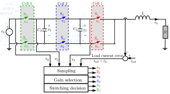
Figure 1.
Topology of flying capacitor three-cell buck converter.
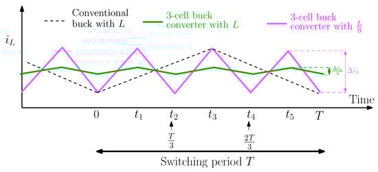
Figure 2.
Inductor current waveforms for the conventional buck converter with a switching period T and inductance L and two different inductor choice for the 3-cell buck converter operating at the same switching period.
Each pair of switches and indicates a cell. Switches and diodes are activated in a complementary manner. When is on, is off and viceversa. The voltages in the cells must be balanced to reduce the stress in these devices [2,3]. The presence of switching devices in power electronic converters produce a cyclic change of structure when defined conditions of time and variables are fulfilled. The different switch positions define the different circuit configurations among which the converter toggles depending on the values of , and . The triple subscript notation that was adopted in this study correspond to the state of the different switches that is in turns related to the values the command signals . Namely, defines the state of the switches for . If , is closed (on) and if , is open (off). For instance the state (1,1,1) for the switches , and defines configuration for which all the switches are closed and the state for the same switches defines configuration for whic all the switches are open. For optimization of the state variable ripples, the driving signals are phase shifted [2]. The switching from one configuration to the following forms a fixed sequence as according to the operation modes. Each configuration is described by an affine time invariant differential equations in the form of . and are the system matrices and vectors during each configuration for all the possible combinations of the values of for for a specific mode of operation. is the vector of state variables , and . The mathematical model can be obtained by applying standard Kirchhoff’s voltage and current laws hence obtaining the following set of continuous-time differential equations modeling the dynamics of the converter
It is worth noting here that the switched model is piecewise affine and for each different configuration, the corresponding differential equation can be solved in closed form.
2.2. Operating Mode under Study
The three-cell buck converter has different operating modes that depend on the value of the steady-state duty cycle D of the switches . It should be noted here that D is the same for all the switches . This study was carried out with the condition . The same procedures can be followed for other ranges of D. The driving signals sequence is given by as depicted in Figure 3. It develops a periodic orbit with six configurations per switching cycle. The sequence is shown as follows
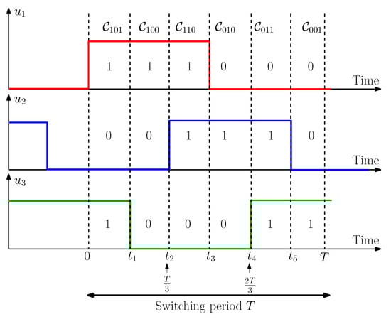
Figure 3.
Driving signals for .
The current paths in each circuit configuration are highlighted in Figure 4. The matrices , the vectors for each topology and a brief description of the behavior in the converter elements for each case are shown in Table 1.
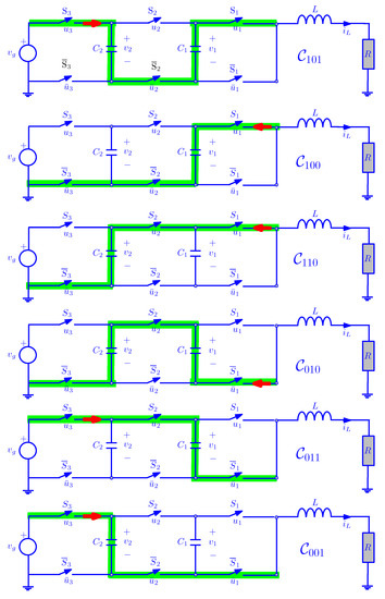
Figure 4.
Configurations used by the flying capacitor three-cell buck converter for steady-state duty cycle in the range . Green color indicates the current path and the red arrows stands for power flow direction.

Table 1.
Matrices for the eight different configurations.
2.3. Discrete-Time Controller
Power electronic converters are generally used to provide a desired voltage/current for the load. This can be accomplished through suitable feedback loops. For flying capacitor multi-cell converters, the controller task it to regulate the voltage/current of the load and also to balance the flying capacitor voltages to effectively reduce the switches voltage stresses. It can be demonstrated that if the duty cycles for all the cells is the same, a natural balancing phenomenon takes place without using the flying capacitor voltages in the feedback loop [34]. However, the transient response speed in this case depends on the circuit parameters and could not undesirably very slow. To avoid this problem, the voltages of the cell are also used in the feedback loop. The controller must be able to regulate the current and balance the input voltage between the different cells. The expression of the duty cycles in terms of the state variables error can be fixed according to the control objectives. A purely proportional control will be used here with the aim to minimize the error between the current and voltages and their references values. As the system contains three controlled switches, three different duty cycles must be generated and their corresponding driving signals must be applied for the three switches. The error between the controlled outputs and their references are appropriately combined and used in a discrete time modulation strategy. In particular, the inductor current (which is also the load current) is controlled to a desired current reference and the flying capacitor voltages and are controlled to and of the input voltage respectively. The charge and discharge of the capacitors depend on the flow direction of the current across it. The discrete-time duty cycles are given by
where , and are feedback coefficients and stands for the sampled state variable at time instant , . The duty cycles are decided periodically based on the samples of the state variables at each start of switching period. For that, one sample of the state variables per period is used. It is worth to note that the duty cycles () are defined as the ratio between the fraction of the switching period T during which the switch is closed (on state) and this period and therefore they must be constrained between 0 and 1. This means that they can be saturated to 0 or to 1 if the expressions in (3)–(5) give a value outside the interval . Therefore, a saturation function must be used to limit the value of in this interval. The final expressions for the duty cycles are
where is the saturation function defined as follows
The driving signals are appropriately phase-shifted in such a way that the signal is high and the switch is closed (on) during the time interval , the signal is high and the switch is closed (on) during the time interval while the signal switch is closed (on) during the time interval , where T is the constant switching and sampling period. Three of the switching instants will be given in a fixed pattern according to the values of , and . These are , and . This fixed pattern switching is due the phase shift between the driving signals (). The other remaining switching instants are , and . For stability analysis the operation during only one period is needed. During one switching period, These are , and , , and .
3. Nonlinear Behavior from Time-Domain Numerical Simulations
Our concern in this section is to present some graphic results to support and complement the study. The fixed parameter values used in this study are depicted in Table 2. The parameters and are varied. A powerful tool to have a wide panoramic view of the different dynamical behavior that the system can have when parameters are varied is a bifurcation diagram. In order to explore the dynamics of the system, bifurcation diagrams for the system are plotted by considering the current feedback gain as bifurcation parameter which is varied within the range A−1 for two different values of A (25 kW) and A (64 kW) respectively. The bifurcation diagrams are obtained by sampling the vector of state variables at the switching period thus yielding , . The transient samples are eliminated and the last 200 samples are considered as steady-state. The inductor current is plotted as the bifurcation parameter is varied. The results are shown in Figure 5. It can be observed that we get qualitatively similar bifurcation at the onset of instability independently of the value of . Let us take the bifurcation diagram in the left panel of Figure 5 as an example. From this figure, it is possible to see that the system exhibits a stable periodic behavior for values of less than a critical value A−1. At this critical value of the feedback gain, the system period-1 limit cycle loses its stability and the attractor of the system evolves on a period-2 limit cycle, i.e., the system undergoes a period doubling bifurcation and a period-2 limit cycle emerges. By further increasing the feedback gain , the resulting period-2 limit cycle undergoes a period doubling resulting in a period-4 limit cycle. For higher values of , the system undergoes more bifurcations phenomena leading eventually to chaotic behavior. Nonlinear behavior manifested by different periodicity parametric windows and chaos can also be observed.
Table 2.
The fixed parameter values used in numerical simulations.
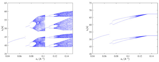
Figure 5.
Bifurcation diagrams from the exact switched model implemented in PSIM© software taking as a bifurcation parameter. Left: A (25 kW). Right: A (64 kW).
In order to check the results obtained from the previous bifurcation diagrams, time-domain simulations have been carried out by using the exact switched circuit-level model implemented in PSIM© software. The steady-state time-domain waveforms are depicted in Figure 6 for different values of . It is worth noting that in the top left panel of Figure 6, the flying capacitor voltages oscillate at the switching frequency kHz, the inductor current oscillate at the double of the switching frequency kHz due to interleaving effect and all the duty cycles are the same and constant in steady-state. In the top right panel of Figure 6, the flying capacitor voltages oscillate at one half the switching frequency kHz, the inductor current oscillate at the switching frequency kHz and all the duty cycles are jumping up and down between two different values one of them is saturated to its lower level 0. In the bottom left panel of Figure 6, the flying capacitor voltages oscillate at one fourth the switching frequency kHz, the inductor current oscillate at one half the switching frequency kHz and all the duty cycles are jumping between three different values two of them are saturated to their lower level 0. Finally, in the bottom right panel of Figure 6, all the state variables and duty cycles are chaotic and saturated upper and the lower values of the duty cycles are reached. It is also worth to note the increase in the current ripple amplitude after losing the stability of the fundamental period-1 limit cycle which could have a damaging effect on the system efficiency and stresses in the switching devices and which also could shorten their lifetime. Therefore, the stability analysis of this limit cycle is of concern both from a theoretical and from a practical point of view.
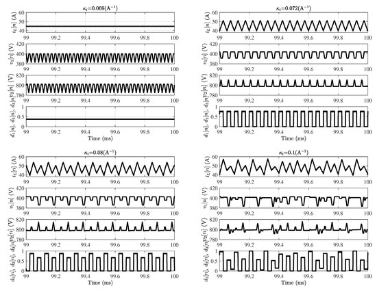
Figure 6.
Time-domain waveforms for different values of that are indicated in each panel title. A.
Floquet theory for limit cycle stability analysis will be applied to predict the onset of instability in the three-cell buck converter. The theoretical background of this theory adapted for the three-cell buck converter is presented in the following section.
4. Theoretical Background for Stability Analysis of Limit Cycles
4.1. Limit Cycles Computation
In steady state, for , there will be six time instants at which a switching from a configuration to another will take place (see Figure 3). These are , and . The other remaining switching instants are , and . The steady-state duty cycle D can be obtained by imposing volt-second balance on the inductor current [1]. This leads to . If , during one switching cycle, the three-cell buck converter changes its structure among the six different configurations shown in Figure 4 and the the system will have a limit cycle using six different affine models. In steady-state, the limit cycle starts with initial conditions , at the start of the switching cycle and evolves according to the switching sequence in (2) as shown below
where and are given by
It is worth to note that the limit cycle can be determined once its initial state is obtained. This initial state can be computed by imposing T-periodicity hence getting
where and are given by the following expressions
The stability properties for the limit cycle represented by the vector can be revealed by using the monodromy matrix which will be determined below.
4.2. Accurate Stability Analysis Using Floquet Theory
As explained before, the switched model of the system under study is time periodic with the switching period T determining the periodicity of the desired limit cycle whose stability can be performed by using Floquet theory combined with Filippov method [24,25]. The main tool for studying the stability of limit cycles using this theory is the monodromy matrix . This matrix is defined such that the dynamics close to a limit cycle can be expressed as follows
where the overhat stands for small signal variations. The eigenvalues of are called Floquet multipliers and they determine the amount of contraction or expansion close to a trajectory and therefore they can be used to determine the local stability of limit cycles. The limit cycle will be stable if all the Floquet multipliers have modulus less than 1. For piecewice affine systems like the power converter considered in this study, the monodromy matrix can be constructed from the product of the state transition matrices corresponding to each sub-interval and the corresponding saltation matrix [24,25,26,27,28]. For the case of the three-cell buck converter of this study, the monodromy matrix can be written as the product of the state transition matrices and saltation matrices at switching instants between their respective time intervals. Namely, the monodromy matrix can be expressed as follows
Figure 7 shows an illustration of how to construct the monodromy matrix using the state transition and the saltation matrices. The state transition matrices from one switching instant to another are just exponential matrices of the different matrices in the piecewise affine model . The saltation matrices can be obtained by first determining the conditions governing the switching in the previous model. These switching conditions are given by the following expressions
where is the vector of the reference signals that can be expressed by
and , and are the gradients corresponding to the switching functions , . The saltation matrices , , , , and can be obtained using the Filippov method [24,25,28] and their expression are
where is a unitary matrix with appropriate dimension. As stated before, due to interleaving effect, the three switching instants 0, and are given in a fixed pattern and therefore one has
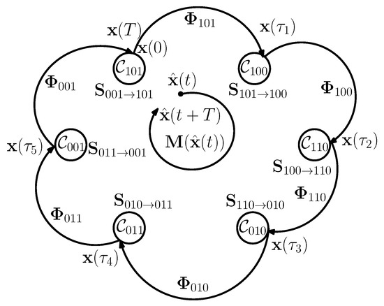
Figure 7.
Transition state diagram between the different configurations and their corresponding matrices.
This implies that
Therefore, expression (11) for the monodromy matrix becomes
To obtain the gradients for , the expression of must be obtained in terms of t for . To get this expression, let us write for in terms of
Therefore, the sampled state can be expressed as follows
where matrix is given by
With the expression of in terms , the gradient vectors become as follows
Finally, the partial time derivative for are
With the previous expressions for all the terms needed for constructing the monodromy matrix, this can be derived and the stability analysis of the limit cycles can be performed. It is worth noting here that the previous theoretical approach can be applied to any kind of limit cycles. These refer to the different periodic orbits under steady state operation. This section considers the period-1 limit cycle which is the only desired behavior for this kind of converters in any industrial application.
On the other hand, although the obtained monodromy matrix is accurate for predicting the onset of instability, it is far from being simple and cannot be applied directly for system design. In the coming subsection an approximate expression for this matrix will be derived. It will allow showing insight into how the different system parameters influence the system dynamics.
4.3. Approximate Expression of the Monodromy Matrix and Stability Region in the Parametric Space
The computational efforts with the previous approach is very high and it also precludes obtaining simple expressions for the stability boundary in the parametric space. In this section, some realistic assumptions will be made in order to obtain simple expressions for the stability borders. These expressions will be validated from numerical simulations using the exact semi-analytical approach detailed previously. A comparison will be performed between the results obtained from the exact approach and those obtained from the simplified approximate approach. The purpose of this comparison is to give a further support to the feasibility of the using the approximate expression of the monodromy matrix for design purposes.
In practice, the switching period is selected much smaller than the time constants of the different converter configurations. Under this condition, it is possible to approximate the matrix exponential as follows . By using this simplified expression, we can obtain an approximate expression for the limit cycles, saltation matrices and finally monodromy matrix. The approximate expression of the limit cycle evaluated at the start of the switching period is given by
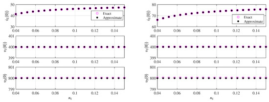
In order to make a validation of the simplified expression of the let us compare the result from both the exact and the approximate approach. Namely, the validity of (39) is first demonstrated before obtaining the approximate expression of the monodromy matrix. Figure 8 shows the evolution of the voltage and the current coordinates of as function of the feedback gain for two different values of the current reference using the exact expression (9) and the approximate one (39). A remarkable agreement can be clearly observed which demonstrates that for design-purposes, the approximate expression (39) can be used without having to use the state exact transition matrices whose computation could be very time consuming in a repetitive simulation process. This also indicates that very little error expected if the stability analysis is performed using an approximate expression for the monodromy matrix.
With the approximated vector given in (39) and the simplified expressions of the state transition and the saltation matrices, the expressions of the monodromy matrix evaluated at the previous limit cycle can be explicitly expressed as follows
Table 3 shows a comparative analysis of the results from the exact and the approximate monodromy matrix. This table shows the limit cycle represented by their initial values , the corresponding Floquet multiplies, the exact and the approximate monodromy matrix and the stability of limit cycles. The values of the Floquet multipliers are obtained by solving the characteristic equation for both cases. As can be observed, the matching between the results is remarkable.
Table 3.
The values of , the Floquet multipliers and stability of the corresponding limit cycles obtained with exact and the approximate approaches for A.
Figure 9 depicts the Floquet multipliers loci when the parameter is varied. The loci was obtained from the exact and the approximate expression of the monodromy matrix. The loci from both the approximate and the exact expressions of the monodromy matrix shows that the critical value of the feedback gain at which one Floquet multipliers crosses the unit circle is which in a perfect agreement with the numerical simulations performed from the switched model and presented in Section 3. For (A−1), all the Floquet multipliers are inside the unit disk hence indicating that the limit cycle is stable. However, at A−1, one Floquet multiplier crosses the unit circle from the point (−1,0) on the complex plane and the system undergoes a flip bifurcation. For , one of the Floquet multiplier is outside the unit disk being real and negative, the period-1 limit cycle becomes unstable. This explains subhamronic oscillations exhibited by the time waveforms and the bifurcation diagrams in Section 3.
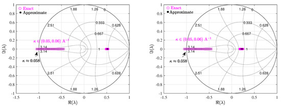
Figure 9.
Floquet multipliers loci from the exact and the approximate expression of the monodromy matrix as the bifurcation parameter is varied for left: A and right: A.
Now that an approximate expression for the monodormy matrix is available in closed form, the Floquet multipliers can be found analytically. The approximate expressions for the Floquet multipliers in terms of system parameters are given by
The approximate closed-form expressions of the Floquet multipliers can be used to determine the stability region of the desired limit cycle in the parameter space. A sufficient condition for stability is that all the Floquet multipliers lie inside the unitary circle. For practical design reasons, the feedback coefficients are restricted within . These limit cycles will be stable whenever the following conditions are fulfilled for the feedback gains , and
The first constraint (44) when evaluated for the set of parameter values of Table 2 gives a critical value of the feedback gain A−1 which is in perfect agreement with the numerical simulations in Section 3. Expressions (44)–(46) can be used to get 2-dimensional diagrams that would help in setting the design limits for the parameters since as they show the safe range of the parameters that would lead to a stable system. The stability boundaries can be plotted in a suitable projection of the parametric space. The parameters can be selected in this space for obtaining a desired response for the system under step type change of a certain reference. For instance, based on a small-signal analysis, the feedback gains that leads to a deadbeat response [42], characterized by the fact that all Floquet multipliers are zero, are given by the following expression
The intersection of the different curves representing (47)–(49) would lead to deadbeat response. Figure 10 shows the constraints (44), (47) and (48) in the parameter space. The stable and the unstable region as well as the set of parameter values leading to a deadbeat response are shown in the same figure. The system parameters are selected on the intersection point, and since the system is of order three, the system will settle within three switching periods after a disturbance takes place. The stable and the unstable region as well as the set of parameter values leading to a deadbeat response are shown in the same figure.
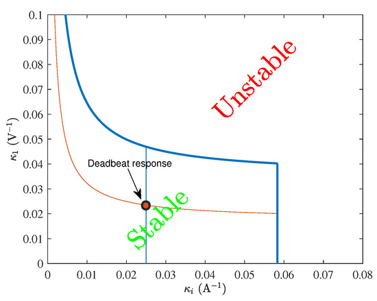
Figure 10.
Stability region and optimum deadbeat response position in the parametric space.
The left panel of Figure 11 shows the Floquet multipliers locus when the parameters are selected at the deadbeat response point in Figure 10. These multipliers are obtained from both the exact and the approximate monodromy matrix. As can predicted by the theoretical analysis, all the multipliers are located at the origin of the complex plane. The matching between the results in this particular case is also remarkable. The right panel of Figure 11 shows the corresponding system response to a 5% step change in the input voltage with the feedback. It can be observed that the duration of the transient after a perturbation in the input voltage takes place is three periods agreed with the theoretical prediction.
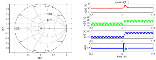
Figure 11.
Deadbeat response of the system. Left: The Floquet multipliers are at the origin of the comlpex plane. Right: The system settling time is three switching periods.
5. Conclusions
Power electronics converters are intrinsically complex nonlinear dynamical systems. Under parameter changes, undesired nonlinear behavior in the form bifurcations and subharmonic oscillation may take place. Understanding the nonlinear behavior and determining the effect of parameters in these systems could help in their design process. The first challenge to understand and to study these systems is obtaining an accurate model that can predict the behavior of such complex systems. Like other conventional power converters, multi-cell flying capacitor converters may also exhibit undesired nonlinear behavior in the form of bifurcation phenomena that could take place for some parameter values. First an accurate model has been used for numerically simulating the system behavior and predicting the nonlinear behavior of a three-cell flying capacitor buck converter under a discrete-time controller. In particular, bifurcation diagrams for the system under this controller has been computed. Floquet theory is a powerful tool to analyze and predict nonlinear behavior in this kind of systems. We have illustrated the use of the theory by studying a three-cell flying capacitor buck converter under discrete-time controller. First we have analyzed the switched nonlinear model of the system. Using Floquet theory, the expression of the monodromy matrix has been used to reveal the effect of suitable parameters on the system. However, the exact expression of this matrix gives little insight out the impact of each system parameter. Under some conditions, the monodromy matrix can be approximated by a simple expression whose validity has been demonstrated by numerical simulations. The simplified expression was used leading to very similar results than the ones obtained by the exact expression of the monodromy matrix. In particular, the critical value of parameters at which instability takes place using the exact monodromy matrix model were shown to be very similar to the ones obtained by an approximate expression of this matrix. The advantage of this latter is that it hows insight into how the different system parameters influence its dynamical behavior. We used the expression of this matrix to determine analytically the limit cycles, their stability status and the onset of their bifurcation. Using the simplified expression of the monodromy matrix, the stability boundaries can be easily plotted in terms of suitable parameters such as the feedback gains, input voltage, load resistance, switching frequency, filter inductance and flying capacitor capacitance values. Finally, a deadbeat-based tuning of the controller gains was used that has lead to a response with minimum settling time after a step change in system parameters. Therefore, the deep understanding of the nonlinear dynamics of the converters has allowed a design of the system with an optimum dynamic response as illustrated by simulation results from the nonlinear switched model of the converter.
Author Contributions
These authors contributed equally to this work. All authors have read and agreed to the published version of the manuscript.
Funding
The authors would like to acknowledge The support by the Spanish Ministerio de Economia y Competitividad under grants DPI2017-84572-C2-1-R. A. El Aroudi and M. Al-Numay acknowledge financial support from the Researchers Supporting Project number (RSP-2020/150), King Saud University, Riyadh, Saudi Arabia.
Conflicts of Interest
The authors declare no conflict of interest.
References
- Erickson, R.W.; Maksimovic, D. Fundamentals of Power Electronics; Springer: Berlin/Heidelberg, Germany, 2001. [Google Scholar]
- Meynard, T.A.; Fadel, M.; Aouda, N. Modeling of Multilevel Converters. IEEE Trans. Ind. Electron. 1997, 44, 356–364. [Google Scholar] [CrossRef]
- Meynard, T.A.; Foch, H.; Thom, P. Multicell Converters: Basic concepts and Industry Applications. IEEE Trans. Ind. Electron. 2002, 49, 955–964. [Google Scholar] [CrossRef]
- El Aroudi, A.; Debbat, M.; Martinez-Salamero, L. Poincaré maps modeling and local orbital stability analysis of discontinuous piecewise affine periodically driven systems. Nonlinear Dyn. 2007, 50, 431–445. [Google Scholar] [CrossRef]
- Deane, J.H.B.; Hamill, D.C. Instability, subharmonics and chaos in power electronic systems. IEEE Trans. Power Electron. 1990, 5, 260–268. [Google Scholar] [CrossRef]
- Tse, C.K. Flip bifurcation and chaos in three-state boost switching regulators. IEEE Trans. Circuits Syst. I Fundam. Theory Appl. 1994, 41, 16–23. [Google Scholar] [CrossRef]
- Tse, C.K. Chaos from a Buck switching regulator operating in discontinuous mode. Int. J. Cir. Theor. Appl. 1994, 22, 262–278. [Google Scholar] [CrossRef]
- Wolf, D.; Verghese, M.; Sanders, S.R. Bifurcation of Power Electronic Circuits. J. Frankl. Inst. 1994, 331B, 957–999. [Google Scholar] [CrossRef]
- Chakrabarty, K.; Poddar, G.S.; Banerjee, S. Bifurcation behavior of the buck converter. IEEE Trans. Power Electron. 1996, 11, 439–447. [Google Scholar] [CrossRef]
- Fossas, E.; Olivar, G. Study of chaos in the Buck converter. IEEE Trans. Circuits Syst. 1996, 43, 13–25. [Google Scholar] [CrossRef]
- di Bernardo, M.; Garofalo, F.; Glielmo, L.; Vasca, F. Switchings, bifurcations, and Chaos in DC-DC converters. IEEE Trans. Circuits Syst. 1998, 48, 133–141. [Google Scholar] [CrossRef]
- El Aroudi, A.; Benadero, L.; Toribio, E.; Olivar, G. Hopf bifurcation and chaos from torus breakdown in a PWM voltage-controlled DC-DC boost converter. IEEE Trans. Circuits Syst. I Fundam. Theory Appl. 1999, 46, 1374–1382. [Google Scholar] [CrossRef]
- Robert, B.; Robert, C. Border Collision Bifurcations in a One-Dimensional Piecewise Smooth Map for a PWM Current-Programmed H-Bridge Inverter. Int. J. Control 2002, 7, 1356–1367. [Google Scholar] [CrossRef]
- Mazumder, S.K.; Nayfeh, A.H.; Borojevi, D. Theoretical and experimental investigation of the fast- and slow-scale instabilities of a DC-DC converter. IEEE Trans. Power Electron. 2001, 16, 201–216. [Google Scholar] [CrossRef]
- Zhusubaliyev, Z.T.; Soukhoterin, E.A.; Mosekilde, E. Quasi-periodicity and border-collision bifurcations in a DC-DC converter with pulsewidth modulation. IEEE Trans. Circuits Syst. I Fundam. Theory Appl. 2003, 50, 1047–1057. [Google Scholar] [CrossRef]
- Banerjee, S.; Verghese, G.C. Nonlinear Phenomena in Power Electronics—Attractors, Bifurcations, Chaos, and Nonlinear Control; IEEE Press: New York, NY, USA, 2001. [Google Scholar]
- Tse, C.K. Complex Behavior of Switching Power Converters; CRC Press: New York, NY, USA, 2003. [Google Scholar]
- Chua, L.O. Special issue on chaos in electronic systems; tutorial and descriptive articles for the non-specialist. Proc. IEEE 1987, 75, 1022–1032. [Google Scholar]
- Hamill, D. Power electronics: A field rich in nonlinear dynamics. In Proceedings of the Workshop on Nonlinear Dynamics of Electronic Systems, Dublin, Ireland, 28–29 July 1995; pp. 164–179. [Google Scholar]
- El Aroudi, A.; Debbat, M.; Giral, R.; Benadero, L.; Olivar, G.; Toribio, E. Bifurcations in DC-DC switching converters: Review of methods and applications. Int. J. Bifurc. Chaos 2005, 15, 1549–1578. [Google Scholar] [CrossRef]
- El Aroudi, A.; Giaouris, D.; Iu, H.H.; Hiskens, I.A. A Review on Stability Analysis Methods for Switching Mode Power Converters. IEEE J. Emerg. Sel. Top. Circuits Syst. 2015, 5, 302–315. [Google Scholar] [CrossRef]
- El Aroudi, A.; Haroun, R.; Cid-Pastor, A.; Martinez-Salamero, L. Suppression of Line Frequency Instabilities in PFC AC-DC Power Supplies by Feedback Notch Filtering the Pre-Regulator Output Voltage. IEEE Trans. Circuits Syst. I Regul. Pap. 2013, 60, 796–809. [Google Scholar] [CrossRef]
- Kassakian, J.G.; Schlecht, M.F.; Verghese, G.C. Principles of Power Electronics; Addison-Wesley: New York, NY, USA, 1991. [Google Scholar]
- Leine, R.L.; Nijemeijer, H. Dynamics and Bifurcations of Non-Smooth Mechanical Systems; Lecture Notes in Applied and Computational Mechanics; Springer: Berlin/Heidelberg, Germany, 2004. [Google Scholar]
- Giaouris, D.; Maity, S.; Banerjee, S.; Pickert, V.; Zahawi, B. Application of Filippov method for the analysis of subharmonic instability in DC-DC converters. Int. J. Circuit Theory Appl. 2009, 37, 899–919. [Google Scholar] [CrossRef]
- Floquet, G. Sur les équations différentielles linéaires à coefficients périodiques. Ann. Sci. de L’E.N.S. 2eme Ser. 1883, 12, 47–88. [Google Scholar] [CrossRef]
- Aizerman, M.A.; Gantmakher, F.R. On the stability of Periodic Motions. J. Appl. Math. Mech. 1958, 22, 1065–1078. [Google Scholar] [CrossRef]
- Filippov, A.F. Differential Equations with Discontinuous Righthand Side; Kluwer Academic: Dordrecht, The Netherlands, 1988. [Google Scholar]
- Robert, B.; El Aroudi, A. Discrete time model of a multi-cell dc/dc converter: Non linear approach. Math. Comput. Simulat. 2006, 71, 310–319. [Google Scholar] [CrossRef]
- El Aroudi, A.; Robert, B.; Cid-Pastor, A.; Martinez-Salamero, L. Modeling and Design Rules of a Two-Cell Buck Converter under a Digital PWM Controller. IEEE Trans. Power Electron. 2008, 23, 859–870. [Google Scholar] [CrossRef]
- El Aroudi, A.; Angulo, F.; Olivar, G.; Robert, B.; Feki, M. Stabilizing a Two-Cell DC-DC buck Converter by Fixed Point Induced Control. Int. J. Bifurc. Chaos 2009, 19, 2043–2057. [Google Scholar] [CrossRef]
- Kaoubaa, K.; Pelaez-Restrepo, J.; Feki, M.; Robert, B.G.M.; El Aroudi, A. Improved static and dynamic performances of a two-cell DC-DC buck converter using a digital dynamic time-delayed control. Int. J. Circ. Theor. App. 2012, 40, 395–407. [Google Scholar] [CrossRef]
- El Aroudi, A.; Giaouris, D.; Mandal, M.; Banerjee, S.; Al-Hindawi, M.; Abusorrah, A.; Al-Turki, Y. Complex non-linear phenomena and stability analysis of interconnected power converters used in distributed power systems. IET Power Electron. 2016, 9, 855–863. [Google Scholar] [CrossRef]
- Reznikov, B.; Ruderman, A.; Galanina, V. Analysis of Transients in a Three-Level DC–DC Flying Capacitor Converter. Time Domain Approach. Power Electron. Drives 2019, 4, 33–45. [Google Scholar] [CrossRef]
- Patino, D.; Bâja, M.; Commerais, H.; Riedinger, P.; Buisson, J.; Iung, C. Alternative control methods for DC-DC converters. An application to a four-level three-cell DC-DC converter. Int. J. Robust Nonlinear Control 2011, 21, 1112–1133. [Google Scholar] [CrossRef]
- Asmarashid, B.P.; Koichi, M.; Koji, O.; Jun-ichi, I. Size Reduction of DC-DC Converter using Flying Capacitor Topology with Small Capacitance. IEEE J. Ind. Appl. 2014, 3, 446–454. [Google Scholar]
- Abdelhamid, E.; Corradini, L.; Mattavelli, P.; Bonanno, G.; Agostinelli, M. Sensorless Stabilization Technique for Peak Current Mode Controlled Three-Level Flying-Capacitor Converters. IEEE Trans. Power Electron. 2020, 35, 3208–3220. [Google Scholar] [CrossRef]
- Bonnano, G.; Agostinelli, M.; Corradini, L.; Eslam, A.; Mattavelli, P. Digital Predictive Current-Mode Control of Three-Level Flying Capacitor Buck Converters Flying Capacitor Balancing in a Multi-Level Voltage Converter. U.S. Patent 10,686,370, 16 June 2020. [Google Scholar]
- Abdelmoula, M.; Robert, B. Bifurcations and Chaos in a Photovoltaic Plant. Int. J. Bifurc. Chaos 2019, 29, 1950102. [Google Scholar] [CrossRef]
- Koubaâ, K.; Feki, M. Discrete-time modelling and behaviour analysis of an N-cell DC/DC buck converter. Int. J. Eng. Syst. Model. Simul. 2016, 8, 54–64. [Google Scholar] [CrossRef]
- Gkizas, G.; Giaouris, D.; Pickert, V. A new method on the limit cycle stability analysis of digitally controlled interleaved DC–DC converters. Control Eng. Pract. 2019, 9, 111–122. [Google Scholar] [CrossRef]
- Ogata, K. Discrete-Time Control Systems, 2nd ed.; Prentice Hall: Minneapolis, MN, USA, 1995. [Google Scholar]


Publisher’s Note: MDPI stays neutral with regard to jurisdictional claims in published maps and institutional affiliations. |
© 2021 by the authors. Licensee MDPI, Basel, Switzerland. This article is an open access article distributed under the terms and conditions of the Creative Commons Attribution (CC BY) license (http://creativecommons.org/licenses/by/4.0/).