An Experimental Investigation of Turbulence Features Induced by Typical Artificial M-Shaped Unit Reefs

Abstract

Artificial reefs are considered to have the function of repairing and improving the coastal habitat and increasing the fishery production, which are mainly achieved by changing the regional hydrodynamic conditions. The characteristics of flow turbulence structure are an important part of the regional hydrodynamic characteristics. Different methods are used to evaluate the performance of artificial reefs according to their shape and the purpose for which the reef was built. For this study, the M-shaped unit reefs, which are to be put into the area of Liaodong Bay, were selected as the research object and have never been fully investigated before. Experimental tests were conducted to assess the effect of these M-shaped artificial reefs on the vertical and longitudinal turbulent intensity under different hydraulic conditions and geometries, and datasets were collected by using the Particle Image Velocimetry technique implemented within the experimental facility. The distribution and variation characteristics of the turbulence intensity were analyzed, and the main results obtained can confirm that in the artificial reef area, there was an extremely clear turbulent boundary. Furthermore, the area of influence of the longitudinal turbulence was identified to be larger than that of the vertical turbulence, and the position where the maximum turbulence intensity appeared was close to where the maximum velocity was measured. Finally, results demonstrate that low turbulence conditions are typically located in front of the unit reef, the general turbulence area is located within the upwelling zone, and the more intense turbulence area is located between the two M-shaped monocases. These results are extremely important, because they provide the local authorities with specific knowledge about what could be the effect of these M-shaped reefs within the area where they will be implemented, and therefore, specific actions can be taken in consideration with the geometrical setup suggested as an optimal solution within this study.

1. Introduction

In recent years, due to the pollution of offshore environments, their habitat degradation, overfishing activities, and effect generated by the climate change, global marine fisheries have significantly declined [1,2,3,4,5,6,7]. Nowadays, artificial reefs, submerged structures deliberately constructed or placed on the seabed to emulate some functions of a natural reef, are some of the techniques adopted to protect, regenerate, or enhance the population of living marine resources [8]. Over the last decade, artificial reefs have also been considered to be an effective measure to reduce the impact of human activities on coastal ecosystems and increase fishery production, and recent studies have confirmed these properties [9,10,11,12,13,14,15]. The flow fields generated by artificial reefs are considered to be the source of the major benefits that these structures may have on marine environments. By deploying artificial reefs into open biological environments, there will certainly be disruptions to the original smooth flow fields; however, the new currents generated may facilitate salt transport, enriching coastal ecosystems and providing vital sources and an ideal habitat for reef fish [16,17,18]. Different configurations can in fact influence the flows passing through these structures, generating specific currents that could aid the deposition of solid material as well as the exchange of nutrients between multiple layers, with a consequent beneficial aspect for fish expansion [19,20]. Furthermore, these structures may also be used as protection or gathering areas by fish or other organisms, because the gentle and stable eddy currents created on the back of them could support the deposition of nutrients and function as a shield that is useful for avoiding enemies or larger predators [21,22,23,24,25,26,27].

Research on the hydrodynamics of artificial reefs is primarily based on insights obtained within experimental and numerical modeling of different reef types, individual or as a combination of various geometries, and to date, based on the authors’ knowledge, the main scope was to identify characteristics and changes of upwelling and eddy currents induced by these artificial structures [8,28,29,30,31,32,33,34,35,36,37,38]. However, there is a paucity of studies related to the turbulence around these artificial reefs.

Turbulence represents the most effective mixing factor that can be met in nature on small as well as large scales [39]. In coastal areas, turbulence structures affect the chemical and physical interaction between the reefs and the surrounding features [40], and they have a strong impact on the typology of different aquatic organisms that may have dissimilar preferences for either high or low turbulent flow conditions. Therefore, turbulence is considered to be an extremely important factor affecting the larval survival and recruitment of pelagic fish [41,42].

Previous studies on the turbulent characteristics of natural coral reefs confirm that turbulent mixing controls the vertical coupling between the implantation layer and the overlying water, and it determines the vertical transport of heat, food, pollutants, larvae, or nutrients from the seabed community [40,43,44,45]. At the same time, an improved understanding of turbulent processes on coral reefs is crucial for the prediction of momentum, energy, and scalar transport, and from an understanding of these basic fluxes, it could be possible to learn more insights about the physics that shape reef ecosystem processes [46,47], sediment suspension and transport [48], and larval settlement on reefs [49]. Many mollusc veligers change their behavior in response to turbulence, and variations in these responses provide clues to whether or how adult habitat structure shapes larval behavior [50]. A study conducted by Fuchs et al. [50] has shown that Oyster larvae (Crassostrea virginica) could enhance their settlement success by moving toward the seafloor in the strong turbulence areas associated with coastal habitats, and the speeds that larvae propelled themselves downward rose steadily with turbulence intensity to several times the terminal fall velocity in still water [50]. Turbulence mixing is the major driver to change the physicochemical characteristics of water column, and it can, for example, not only facilitate oxygen transport from water to surface sediment, but it can also enhance sediment suspension, which is one of the key processes affecting water turbidity and indirectly influencing eutrophication in shallow lakes [51,52]. A previous study completed by Li et al. [53] confirmed that turbulence intensity plays an important role in internal phosphorus release: the results presented demonstrated that strong turbulence caused a reduction of phosphate in the overlying water, oxygen delivery was enhanced under moderate turbulence mixing, and turbulence induced high suspended sediment adsorption, contributing more intensively to phosphorous (P) inactivation [53]. Recent studies [54,55,56] have shown that turbulence may also affect the feeding of marine organisms such as plankton and other fish. Furthermore, turbulent motions in the surrounding flows can be important also for the encounters of aquatic microorganisms and their prey by bringing predators and prey close from time to time and thereby enhancing the probability of capture even without relying on self-induced motions [57,58,59,60,61]. Nevertheless, sometimes, turbulence can also provide organisms with hydrodynamic signals that may be wrongly interpreted as generated by an approaching predator, which may affect their behavior and the energetic cost of swimming [62]. In addition, the presence of turbulence can change the particles’ settling velocity, which subsequently alters the concentration within the suspension layer. Thus, turbulence is an influencing factor for sediment transport and seabed evolution as well [63,64]. Considering all these impacts that turbulence may have in marine environments, it is necessary to further study the turbulent characteristics of flow fields altered by the presence of artificial reefs, because these features, as previously mentioned, are being adopted more frequently for coastal protection, rehabilitation, and restoration.

To achieve this aim and fill this gap identified in the literature, this study focuses on the experimental modeling of M-shaped unit reefs, which are to be put into the typical artificial reef area of Liaodong Bay (China) next to the Bohai Sea (Figure 1). The experimental campaign involved testing different inflow velocities and spacing of these M-shaped unit reefs, and results have been collected using the Particle Image Velocimetry (PIV) method. The characteristics of turbulence intensity and its variation under different flow conditions were then analyzed, and results have been presented to characterize specific turbulent flow features in typical M-shaped unit artificial reefs, which should be taken into consideration in Liaodong Bay, where these structures will be used. Furthermore, outcomes obtained in this study can provide a reference for improving artificial reef configurations, which are in continuous development.

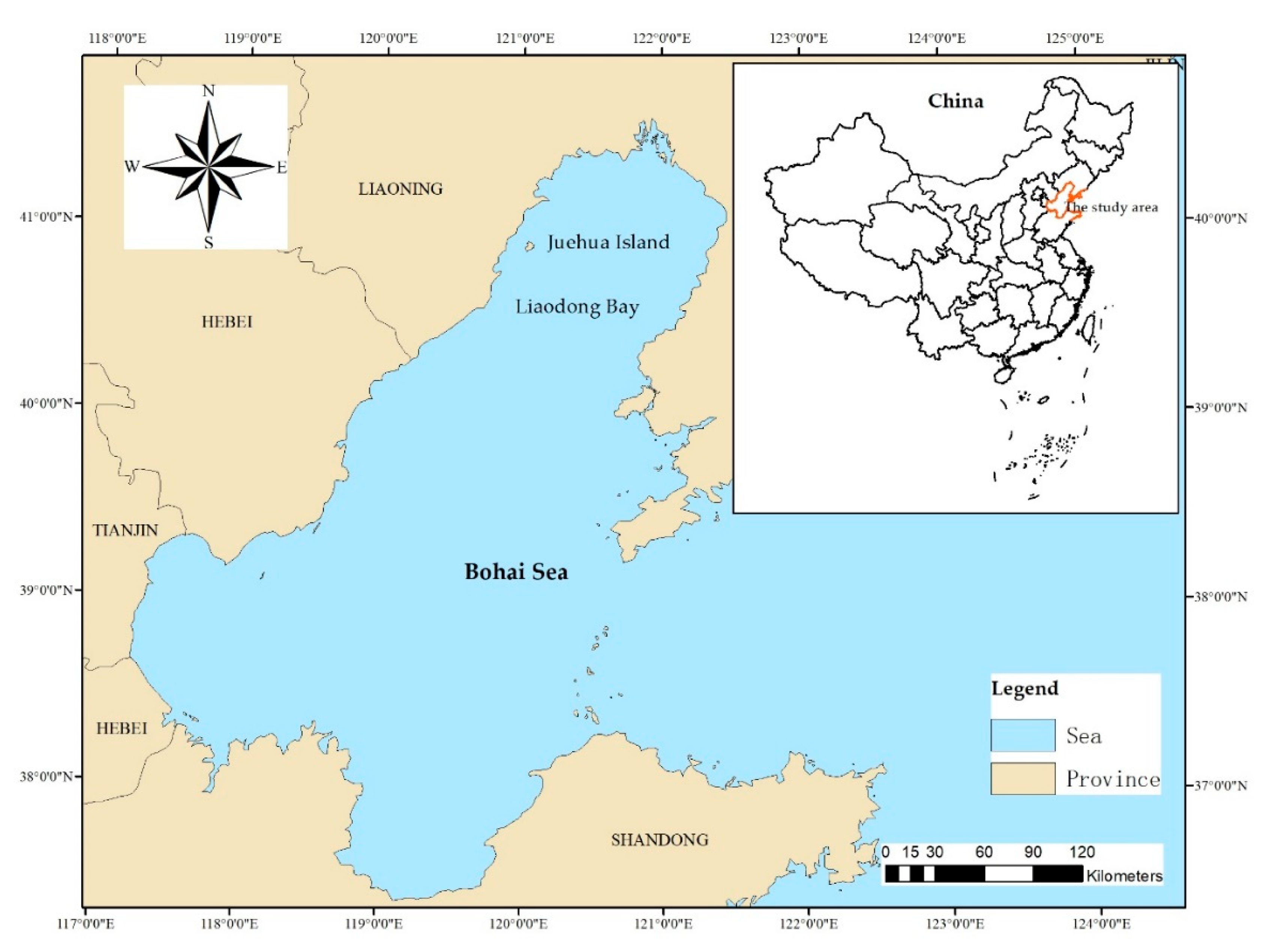
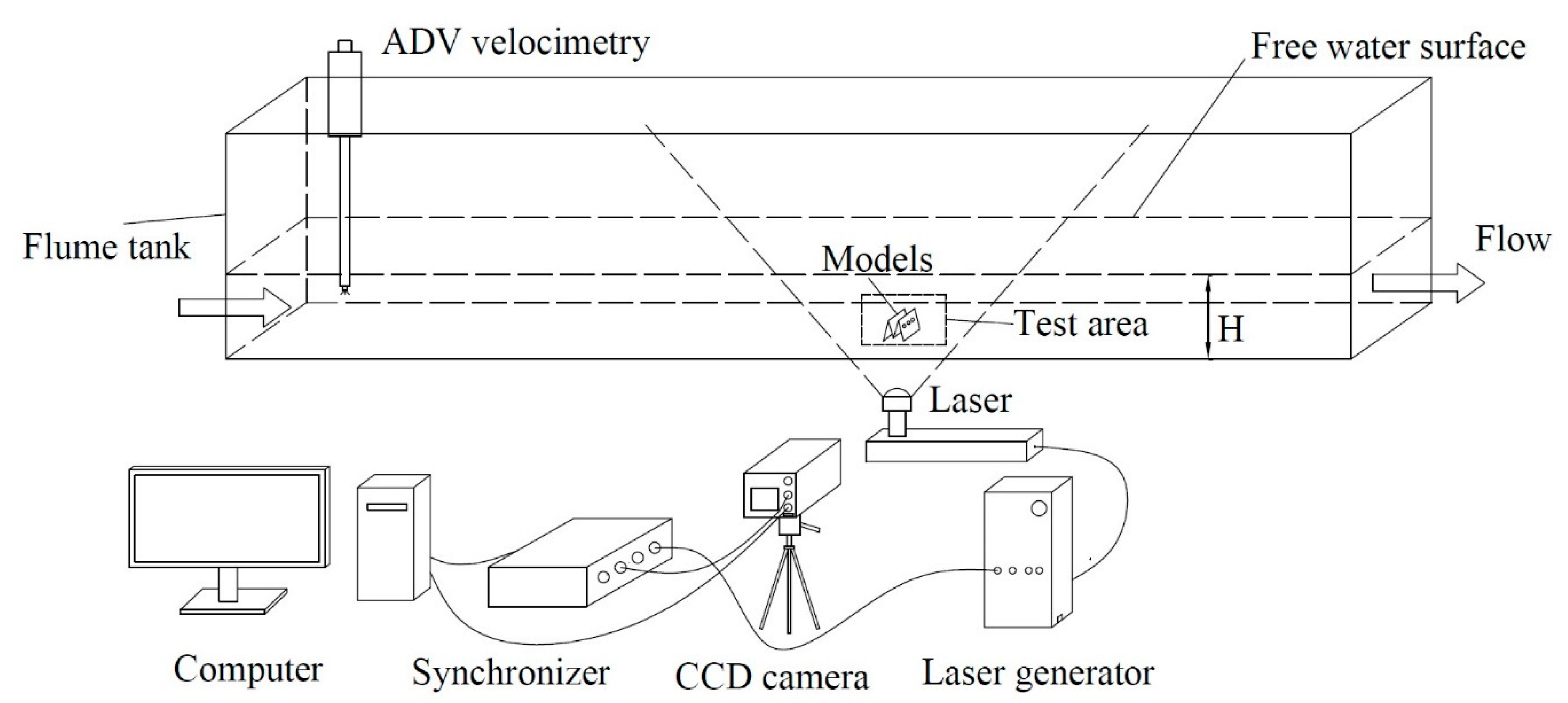
2. Experimental Setup

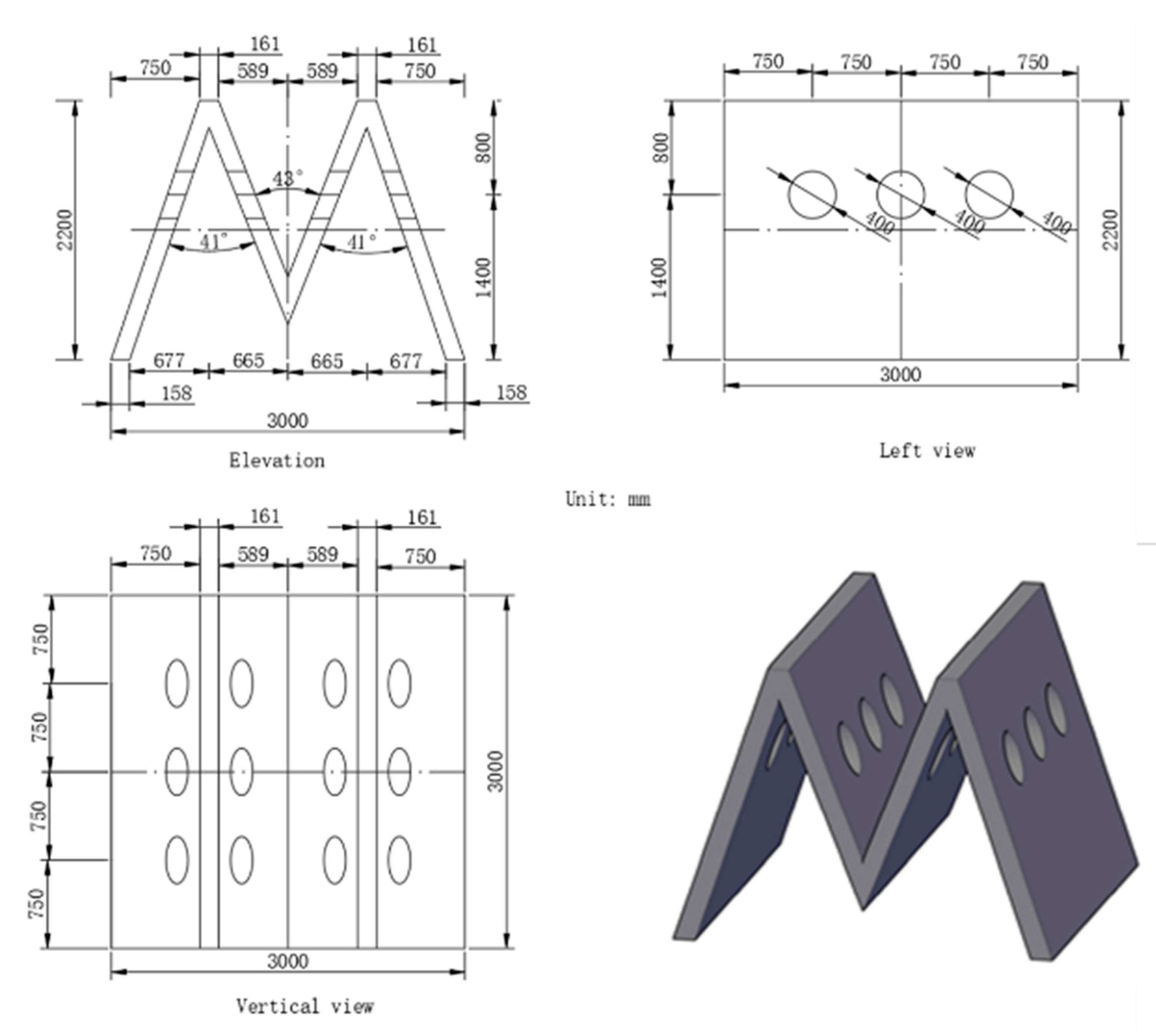
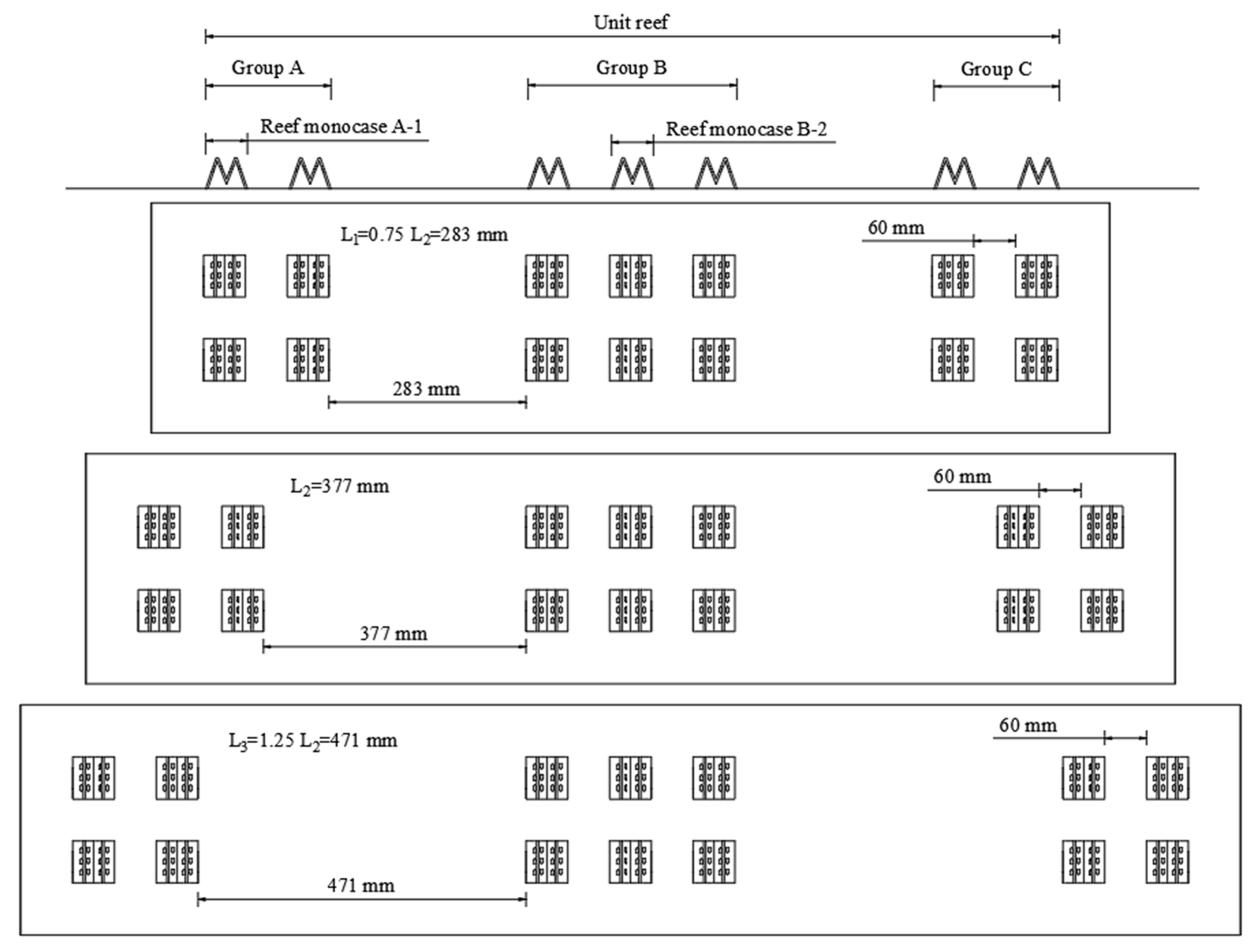
2.1. Experimental Model

The experiments were carried out in a multi-functional flume in the State Key Laboratory of Water Environment Simulation, at Beijing Normal University, China. The internal dimensions of the flume are 25.00 m × 0.80 m × 0.80 m (length × width × height), whose bottom and side are made of transparent glass. The flow is generated by a complete water circulation system, and the maximum flow rate is 240 L/s.

The reef monocase model used for this study is 0.06 m × 0.06 m × 0.044 m in size, 3 mm in thickness, 4 mm in round hole radius, and 4° in triangle angle, which was scaled by a geometric factor of 1:50 according to the prototype size of the M-shaped reef (Figure 2). The field observation of the daily flow velocity reported in the Liaodong Bay varied between 0.6 and 1.8 m/s, which corresponds to a design flow velocity 0.085–0.257 m/s or flow rate 20–60 L/s range according to the scale factor specified here. The M-shaped reef models were made of plexiglass. Each M-shaped unit reef is composed of 14 reef monocases. In order to avoid drifting and rolling, the reef models were fixed on the bottom of the flume with transparent rubber belt and were located perpendicular to the flow direction.

The Particle Image Velocimetry (PIV) method was adopted to investigate flow conditions. This is a non-contact two-dimensional flow field measurement technology based on cross-correlation analysis of flow field images, which can produce a quantitative visualization effect of instantaneous flow patterns without disrupting the phenomena under analysis. It is usually used to support the development of phenomenological models for complex flow or numerical simulation verification. It has become the main experimental technique for measuring flow velocity fields [65,66,67] and has been widely used in the analysis of flow field around artificial reef models in recent years [30,31] as well as for other flow applications [68,69,70,71,72]. The fluid velocity was calculated using an adaptive cross-correlation technique, keeping an interrogation area of 1903.5 × 1183.5 pixels with consideration of 80 pixel overlap between two adjacent areas. Median correction post-processing was applied to remove erroneous vectors, which removed approximately 2 to 7% vectors from each measurement set. To validate this technique, an Acoustic Doppler Current Velocimetry (ADV) was installed 2 m in front of the test target to measure the inflow velocity and results compared with PIV outputs were within the range of 4% error. With the artificial reef model placed in the middle of the flume, the laser used for the PIV data collection was placed at the bottom of the tank to hit the central axis of the reef model. The images were captured by a CCD (Charge Coupled Device) camera and consequently analyzed using Dynamic Studio software [73]. The velocity maps produced were finally visualized using Tecplot software. A full experimental setup is illustrated in Figure 3.

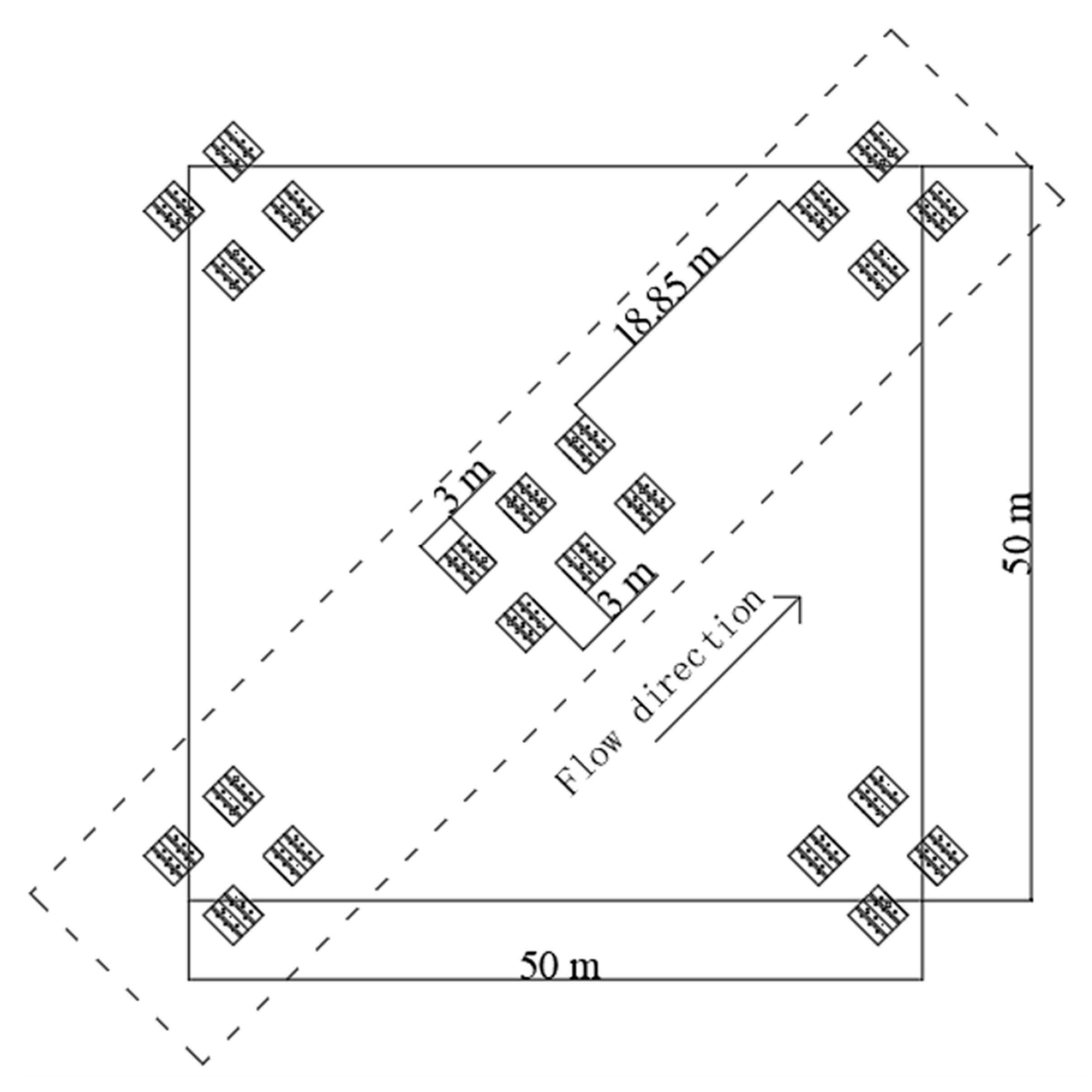
2.2. Experimental Design

The unit reef model is composed of three sub reefs, which are parallel to the flow direction in the prototype arrangement. Along the flow direction, the spacing between each reef monocases group is 18.85 m (Figure 4), which should be 377 mm in the flume experiment according to Froude similarity adopted [30]. On this basis, multiple setups were studied, with the spacing reduced and expanded, replicating different configurations, which were (1) L₁ = 0.75 L₂ = 283 mm, (2) L₂ = 377 mm as the basic spacing typically adopted in the real case scenario, and (3) L₃ = 1.25 L₂ = 471 mm, respectively. According to the study completed by Cui et al. [74], which stated that the most optimal spacing between the two reef monocases should be ≈1.0–1.5 times the length of the reef, the spacing between two monocases in each group was set as one time the model length, which was 60 mm. All the geometrical configurations tested in this study are displayed in Figure 5. Group A, Group B, and Group C correspond to the three sets of artificial reefs, as displayed in Figure 5.

2.3. Hydraulic Conditions

Five velocities measured during a field campaign in the sea area of Juehua Island, where the M-shaped artificial reef prototypes will be released, were selected to be replicated in this study. These velocities are 0.6, 0.9, 1.2, 1.5, and 1.8 m/s, and they were obtained by releasing the flow Q as 20, 30, 40, 50, and 60 L/s, respectively (±2.5%). Based on the Froude similarity adopted, the correspondent experimental velocities tested within the experimental facility were then 0.085, 0.130, 0.170, 0.214, and 0.257 m/s, respectively; therefore, the values replicated were within ±0.86% of the values measured in the field.

The experimental water depth tested in the laboratory was 300 mm, and it was calculated using Froude similarity as well, according to the actual water depth recorded in situ, 15 m. To sum up, a total of 20 groups of experiments were conducted, including four geometrical conditions (1, 2, and 3 previously explained plus a controlled test with no artificial reefs, called 0), and five flow conditions with dissimilar velocities. All these experimental details are summarized and displayed in

Table 1. Testing conditions.

Experimental Group (Test Case)	L (mm)	u0 (mm)	Fr
0 (1–5)	\	0.085–0.257	0.05–0.15
1 (1–5)	283	0.085–0.257	0.05–0.15
2 (1–5)	377	0.085–0.257	0.05–0.15
3 (1–5)	471	0.085–0.257	0.05–0.15

Note: L: the spacing between each artificial reef; u₀: the averaged inflow velocity.

.

3. Methods

3.1. Quantification of Turbulence Velocity

The fluctuating flow structure mainly refers to the distribution of turbulence intensity, which is an important index commonly used to describe the characteristics of turbulent flow fields.

The velocity of each point in the turbulent flow changes with time, but if considering a long time duration, its time-averaged value is relatively stable. Therefore, the time-averaged velocity can be calculated as follows:

$$Time-averagedvelocity\hspace{0.33em}\hspace{0.33em}\hspace{0.33em}\hspace{0.33em}\hspace{0.33em}\hspace{0.33em}\hspace{0.33em}\hspace{0.33em}\overline{u}=\frac{1}{N}{\displaystyle {\sum }_{i=1}^N{u}_i}$$

(1)

The value obtained by subtracting the instantaneous velocity from the average velocity at a point is the fluctuating velocity, also known as turbulence velocity, which is one of the most important characteristics of flow turbulence.

$$Turbulencevelocity\hspace{0.33em}\hspace{0.33em}\hspace{0.33em}\hspace{0.33em}\hspace{0.33em}\hspace{0.33em}\hspace{0.33em}\hspace{0.33em}{u}_{mi}=u_i-\overline{u}$$

(2)

In Equations (1) and (2), u_i is the longitudinal instantaneous velocity at point i; u_mi is the longitudinal turbulence velocity; and N is the number of sampling statistics. The expressions of vertical velocity v_i are similar.

3.2. Quantification of Turbulence Intensity

Turbulence velocity may have positive–negative points, which is not convenient for statistical comparison.

In order to compare the intensity of turbulence at different points more intuitively, the root mean square of turbulent velocity is usually used to represent the intensity of turbulence. Thus, mean square velocity and turbulence intensity are calculated as follows:

$$Meansquarevelocity\hspace{0.33em}\hspace{0.33em}\hspace{0.33em}\hspace{0.33em}\hspace{0.33em}\hspace{0.33em}\hspace{0.33em}\hspace{0.33em}\overline{{u^{\prime }}^2}=\frac{1}{N}{{\displaystyle {\sum }_{i=1}^N\left(u_i-\overline{u}\right)}}^2$$

(3)

$$Turbulenceitensity\hspace{0.33em}\hspace{0.33em}\hspace{0.33em}\hspace{0.33em}\hspace{0.33em}\hspace{0.33em}\hspace{0.33em}\hspace{0.33em}\hspace{0.33em}\hspace{0.33em}\hspace{0.33em}\hspace{0.33em}\hspace{0.33em}\hspace{0.33em}\hspace{0.33em}\hspace{0.33em}{\sigma }_u=\sqrt{\overline{{u^{\prime }}^2}}$$

(4)

The turbulence intensity is usually treated to make it dimensionless. For example, the relative turbulence intensity ${{\sigma }^{\prime }}_u=\frac{{\sigma }_u}{u_0}$ is used to represent the turbulence intensity of the flow, where u₀ is the inflow velocity (the turbulence intensity mentioned below is the relative turbulence intensity).

3.3. Estimation of Reynolds Shear Stress

Reynolds shear stress is the shear stress between the flow layers due to the water momentum exchange and can be quantified as follows:

$$Reynoldsshearstress\hspace{0.33em}\hspace{0.33em}\hspace{0.33em}\hspace{0.33em}\hspace{0.33em}\hspace{0.33em}\hspace{0.33em}\hspace{0.33em}{\tau }_{u\nu }=-\rho \overline{u^{\prime }{\nu }^{\prime }}$$

(5)

As for the turbulence intensity, the Reynolds shear stress is also usually treated to make it dimensionless. For example, the relative Reynolds shear stress $R=\frac{\overline{u^{\prime }{\nu }^{\prime }}}{u_0^2}$ is used to represent the Reynolds shear stress on the XY plane.

4. Results and Discussion

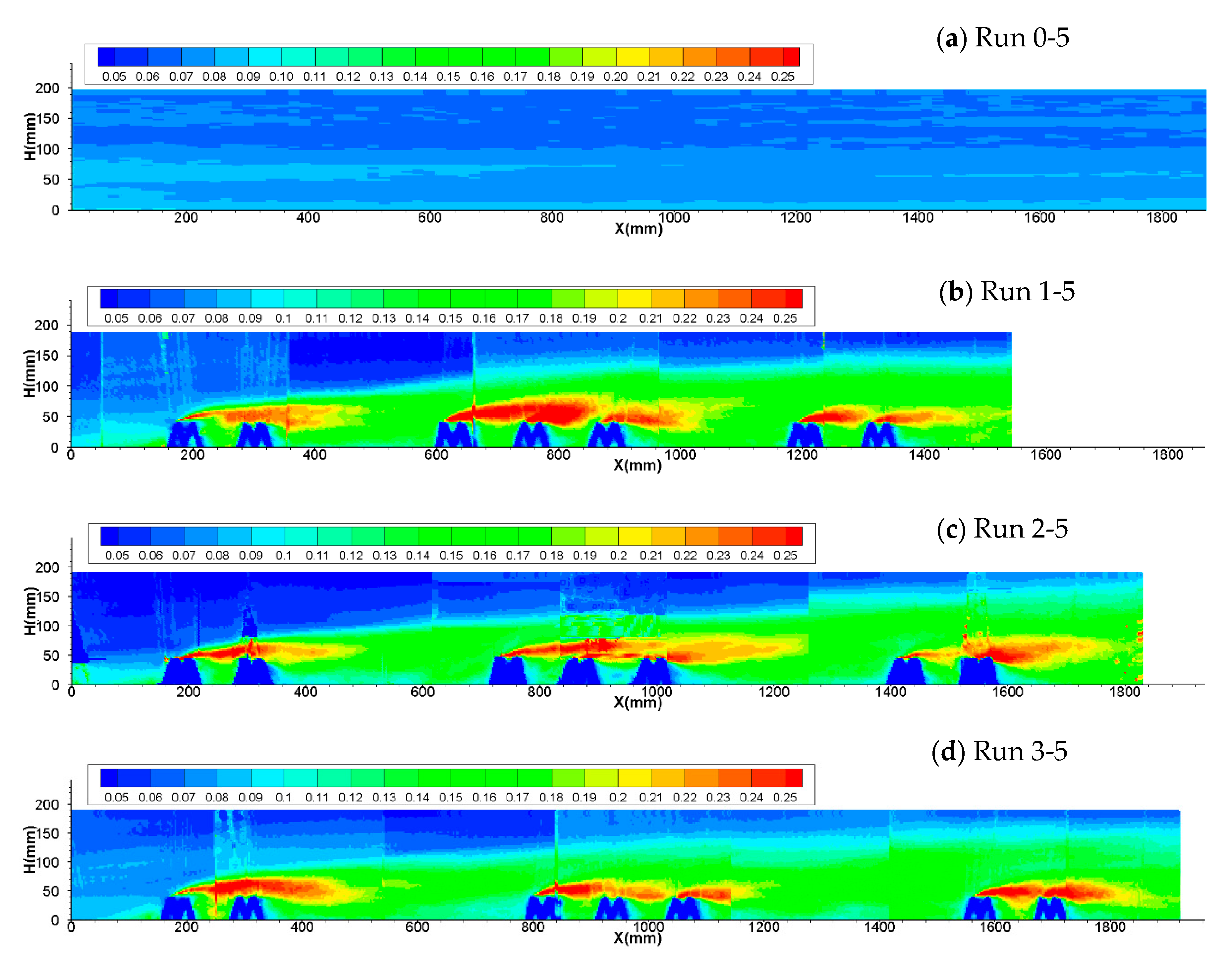
4.1. Characteristics of Turbulence Intensity Distribution along the Flow Direction

The changes of turbulence intensity in the proximity of the unit reef tend to be consistent under different working conditions, as displayed in Figure 6 and Figure 7, which show the distribution of turbulence intensity under the worst scenario for the velocities tested and each geometrical setup; therefore, tests 0-5, 1-5, 2-5, and 3-5 displayed in

Table 2. The average longitudinal and vertical turbulence intensity for cases 0-5, 1-5, 2-5, and 3-5.

Test ID	Average Longitudinal Turbulence	Average Vertical Turbulence
0-5	0.075	0.046
1-5	0.117	0.086
2-5	0.110	0.073
3-5	0.118	0.084

show the average values for the longitudinal and vertical turbulence intensity over the whole study range.

Figure 6 and Figure 7 show that, except for condition 0-5, where no artificial reef is applied, the turbulence intensity has an obvious boundary between the turbulent and non-turbulent regions, which gradually rises with the flow direction. When the flow was introduced into the flume inlet and passed through the artificial reef structure, it was apparent that the flow patterns in the upstream area of the flume and in those around the reef group A, the initial set of artificial reefs, were largely similar despite using different reef configurations. These were understandable as initial flow conditions and are usually typical of each artificial reef shape used. It can be noticed that comparing the same geometrical configuration, the longitudinal turbulence intensity is significantly larger than the vertical one, in terms of magnitude and areas characterized by high values. In fact, the characteristic length of the larger longitudinal turbulence intensity (>2.0) is about 5–7 times the height of the reef, while the larger vertical turbulence intensity (>0.16) is about 2–4 times the height of the reef. Moreover, the location of the area with larger longitudinal turbulence intensity is higher than that of the vertical turbulence intensity, as expected.

Before entering the reef area, the longitudinal turbulence intensity gradually increases from the bottom at about 2.8 times the height of the reef in front of it, and along the flow direction, the turbulence height increases, which is close to the position where the current uplifts. The vertical turbulence intensity begins to change from the bottom at about 1 time the length in front of the reef. These results indicate that the blocking effect of artificial reefs is mainly reflected in the longitudinal velocity.

Analyzing the longitudinal turbulence intensity under different working conditions, the magnitude of the numerical values and the area affected can be classified as follows: condition 2-5 > condition 1-5 > condition 3-5, but in terms of average turbulence intensity, this is the final order: condition 3-5 > condition 1-5 > condition 2-5.

Analyzing the vertical turbulence intensity calculated for different geometrical and hydraulics of the worst scenario (higher velocities), the magnitude of the numerical values obtained and the length of the area affected follow this order: condition 1-5 > condition 2-5 > condition 3-5, but in terms of average vertical turbulence intensity, the order changes to condition 1-5 > condition 3-5 > condition 2-5.

If values of longitudinal and vertical turbulence intensity are combined, the performance follows this order: condition 1-5 > condition 2-5 > condition 3-5; that is, L₁ > L₂ > L₃, which indicates that when the spacing is small, the impact of reef on the flow is greater and the turbulence is stronger.

Nevertheless, it can also be observed that due to the presence of the artificial reefs, the whole unit reef area is characterized by a relatively large turbulence intensity. Higher values of turbulence intensity initiate above the reef, following in parallel the flow streamlines and spreading outward with a strip shape, which is obviously greater than the surrounding turbulence intensity. By comparing the turbulence intensity of the three conditions with the control experiment (0-5) focusing on the same areas where the artificial reefs are located, the longitudinal and vertical turbulence intensity increased by 53.6% and 76.8%, respectively.

Table 2 displays the average values of longitudinal and vertical turbulence for cases 0-5, 1-5, 2-5, and 3-5. It is possible to notice that the real scenario, 2-5, has lower values of turbulence in comparison with the spacing configurations suggested with 1-5 and 3-5. Therefore, configurations suggested by the authors (1 and 3) could be more beneficial to fish and the ecology of the reefs, because stronger turbulence could provide more food and nutrients within the entire area under investigation [75].

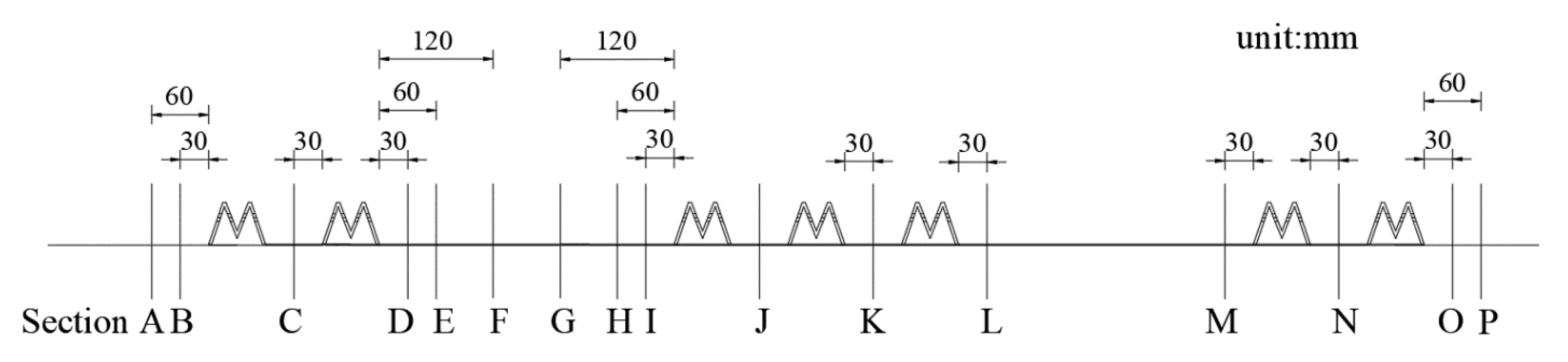
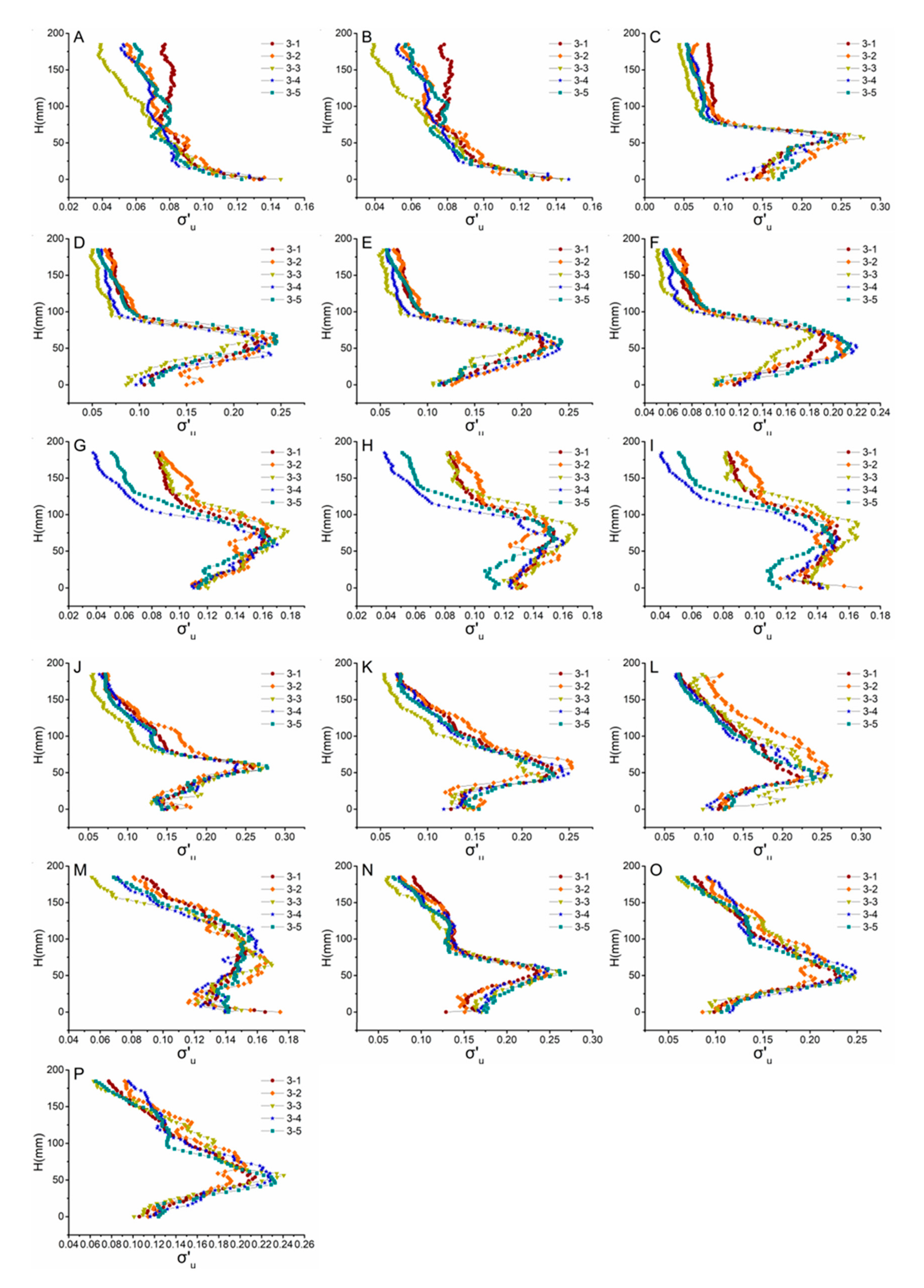
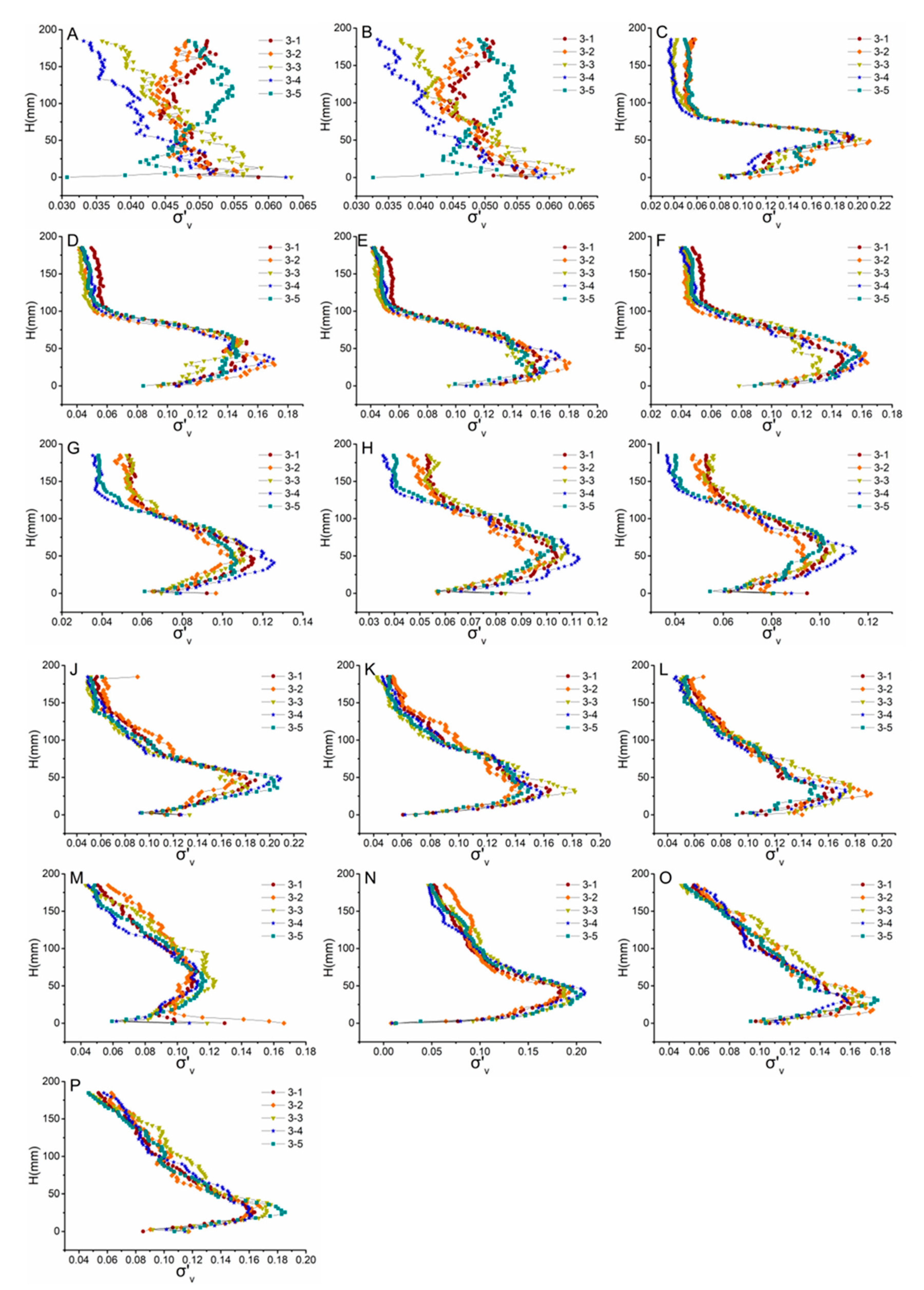
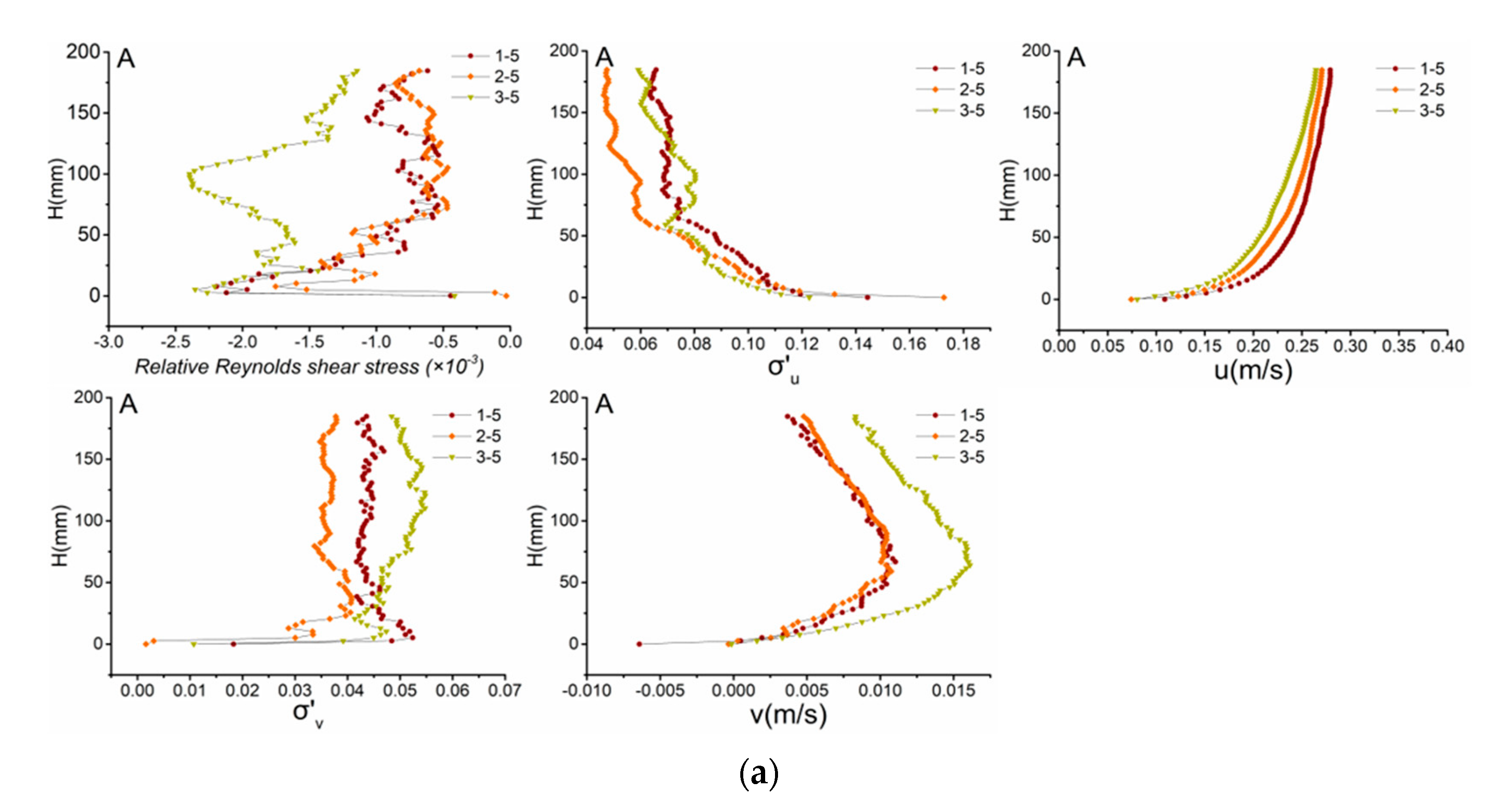
4.2. Characteristics of Turbulence Intensity along the Entire Flow Depth

Although the maps produced for the turbulence within the artificial reefs can clearly show the overall variation of longitudinal and vertical turbulence intensity, due to the difference between unit reef spacing setup for the experiments conducted, it is not convenient to compare and analyze the turbulence intensity at the same relative position because it may be not related to exactly the same location.

In order to accurately compare the changes of turbulence intensity in the vertical line under different velocity conditions, 16 sections were identified as displayed in Figure 8. More in detail, Section A and Section B are 60 mm (1 times reef length) and 30 mm (1/2 times reef length) before the first group (Group A, as introduced in Figure 5) of artificial reefs; Section C is 30 mm after the first monocase of Group A; Section D, Section E, and Section F are 30, 60, and 120 mm after the last monocase of Group A; Section G, Section H, and Section I are 120, 60, and 30 mm in front of the second group of artificial reefs, Group B (as introduced in Figure 5); Section J is 30 mm after the first monocase in Group B; Section K is 30 mm after the second monocase in Group B; Section L is 30 mm after Group B; Section M is 30 mm before the final group of artificial reefs, Group C (as previously displayed in Figure 5); Section N is 30 mm after the first monocase in Group C; Section O and Section P are 30 mm and 60 mm after Group C.

According to the location of these sections relative to the unit reefs, the 16 sections are classified into four categories as follows:

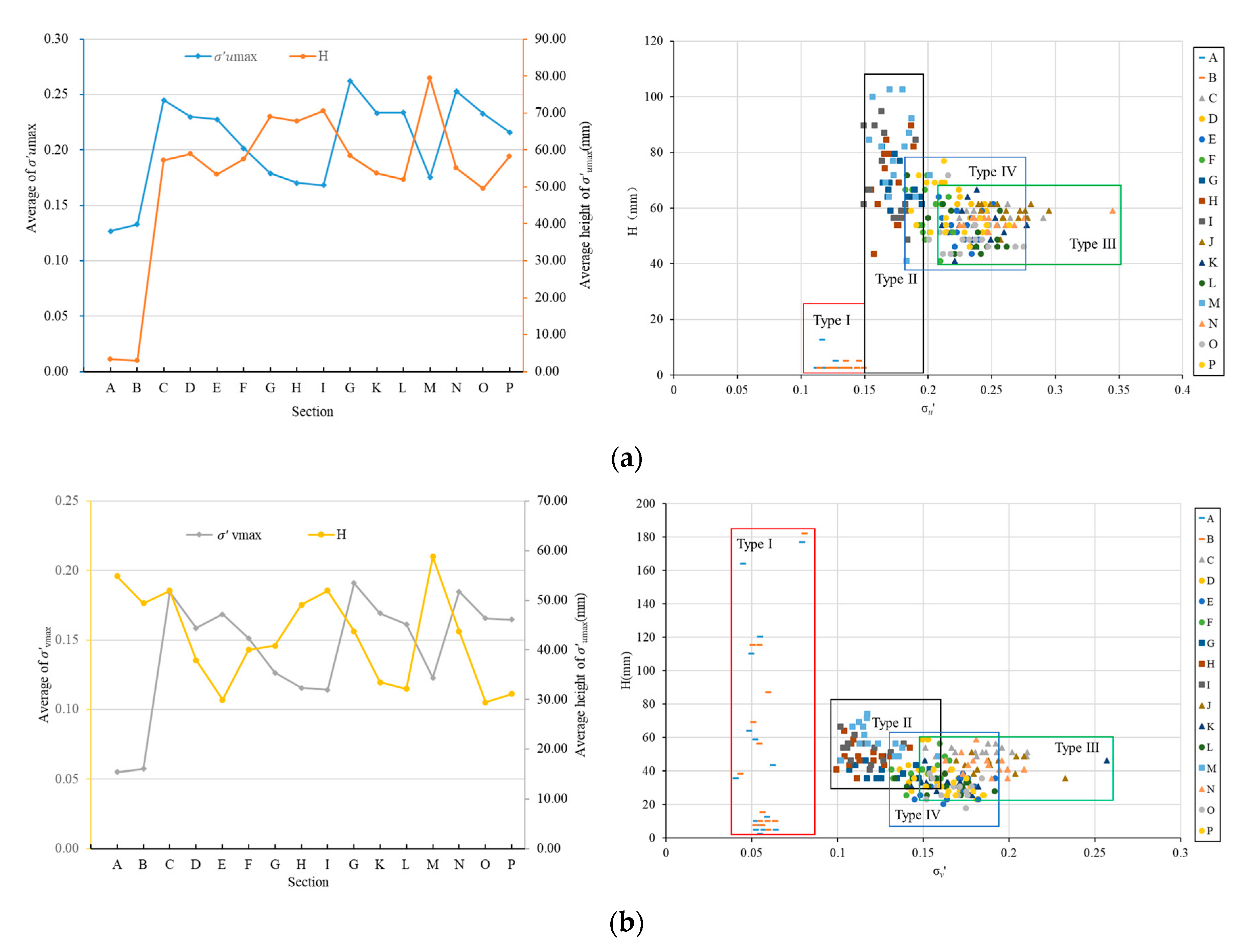
• A and B are the sections not entering the reef area (Type I);
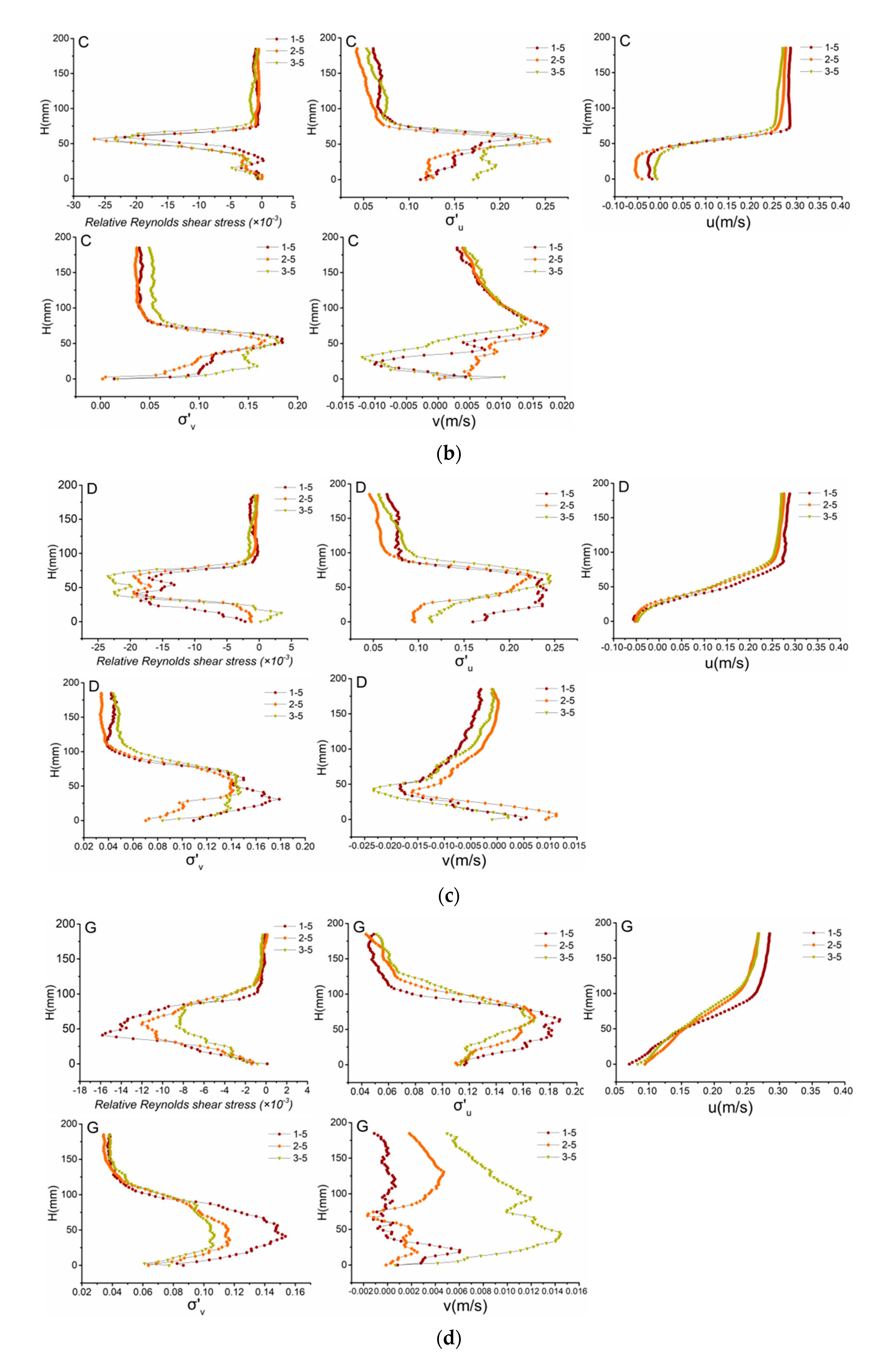
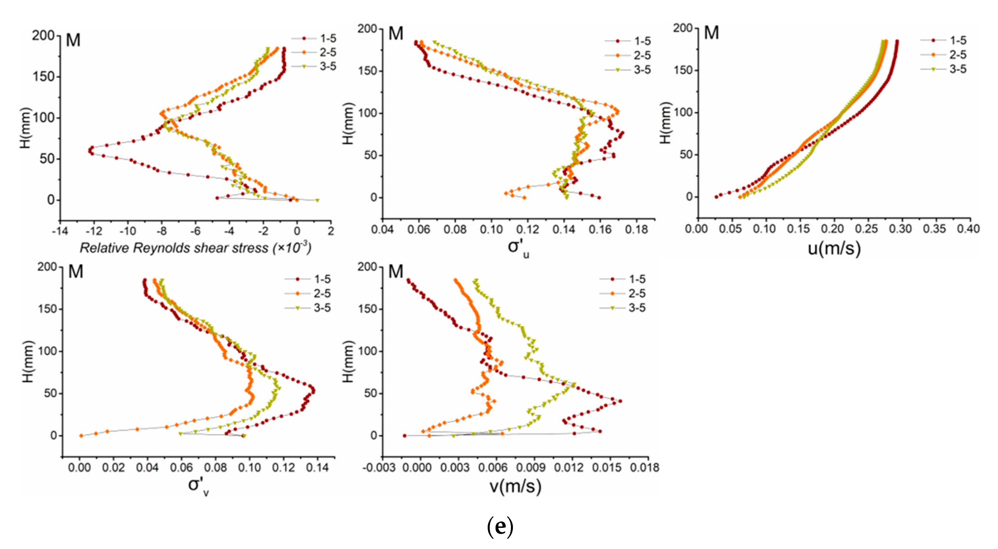
• G, H, I, and M are the front sections of the reef groups (Type II);
• C, J, K, and N are the sections between the two reef monocases (Type III);
• D, E, F, L, O, and P are the rear sections of the reef groups (Type IV).

Figure 9 and Figure 10 show the comparison of longitudinal and vertical turbulence across each section for the worst scenario tested (3) and all the velocities replicated (1–5). It is possible to notice that on the same section, the trends of turbulence intensity are highly coincident, despite the different velocities tested. A general pattern can also be observed: along the flow direction, outside the reef area, the longitudinal turbulence intensity gradually decreases with the increase of the water level, while this behavior cannot be noticed for the vertical turbulence intensity. After the flow enters the reef area, two inflection points appear in the turbulence intensity on the vertical line. In fact, after the flow enters the reef area, the turbulence intensity firstly increases to the maximum value with the increase of water level (1st inflection point); then, it decreases sharply with the increase of water level (2nd inflection point) and then decreases slowly. The 1st inflection point appears at the highest point where the water flow is affected by the reef on the vertical line. In the test area, the height of the 2nd inflection point increases gradually along the flow direction.

At the same time, it was also found that the trend of longitudinal and vertical turbulence intensity is affected by upwelling and back vortex conditions. For example, in sections G, H, I, and M, affected be upwelling, the 1st inflection point of the longitudinal turbulence intensity appears at 1.7 times the reef height, and the position of the 2nd inflection point is not clearly identifiable. The 1st inflection point of the vertical turbulence intensity appears at 1 times the height of the reef, and the 2nd inflection point is higher, about 3.2 times the reef height. However, in the sections affected by back vortex, such as C, J, K, and N, the 1st inflection point of longitudinal turbulence intensity appears at 1.25 times the reef height, and the 2nd inflection point appears at about 2 times the reef height. The 1st inflection point of vertical turbulence intensity appears at about 1 times the reef height, and the 2nd inflection point appears at about 2 times the reef height.

It can be confirmed based on the results displayed in Figure 9 and Figure 10 that the influence of the back vortex on the turbulence intensity is more severe, because the turbulent intensity range of the section in the back-vortex region is larger than that in the upwelling region. However, the influence range of upwelling on turbulence intensity is higher, because the 2nd inflection point of the section in the upwelling region is higher than that in the back-vortex region.

Among the four categories of sections previously identified, we selected one representative section for each type to simplify the comparisons between different locations. Therefore, Section A was selected to represent Type I, Section C was selected for Type II, Section D was selected for Type III, and Section M was selected for Type IV. In addition, G was also included within this list, because it was found that the influence of the front and rear reefs on Section G was similar, and its vertical velocity was quite different under each testing conditions. The vertical distribution of Reynolds shear stress values, longitudinal turbulence intensity, longitudinal velocity, and vertical turbulence intensity and vertical velocity at Sections A, C, D, G, and M are displayed in Figure 11a–e.

It can be highlighted that although there is no direct relationship between the turbulence intensity and the time-averaged velocity, the inflection point of the turbulence intensity on the vertical line is generally consistent with that of the vertical velocity; the minimum Reynolds shear stress appears at a height close to that of the maximum turbulence intensity. Before entering the reef area, the longitudinal turbulence intensity has the following order of magnitude: condition 3-5 > condition 2-5 > condition 1-5. However, after the disturbance of the reef, the turbulence intensity of condition 1-5 with the smallest spacing is the largest. Therefore, it can be stated that small spacing can stimulate the occurrence of turbulent features.

Analyzing the Reynolds shear stress values obtained at each section, when the flow field is not affected by reefs, the Reynolds shear stress is relatively small, and the Reynolds magnitude follows this spacing order: L₂ > L₁ > L₃. After the flow enters the reef area, the Reynolds shear stress changes greatly, and the overall trend is roughly opposite to that of the turbulence intensity: the Reynolds shear stress first decreases to the minimum value with the increase of water level; then, it changes suddenly after encountering the reef. Then, it increases with the rise of water level, and finally, it remains stable, with the overall performance of L₃ > L₂ > L₁. However, there are differences among the different sections: the variation range of Reynolds shear stress in Sections C and D is greater than that in Sections G and M, and the height of the turning point is relatively uniform. The reason for this difference may be that Sections C and D belong to the front part of the reef area and have a blocking effect on the flow. When the flow reaches Sections G and M, the velocity ideally reduced and the turbulence intensity weakens, inducing minor changes to the Reynolds shear stress.

4.3. Characterisation of Maximum Turbulence Intensity

The magnitude and the location of the maximum turbulence intensity can aid in characterizing the effect of the artificial reef on the flow. Figure 12 shows the relationship between the maximum value of turbulence intensity and the height at which it occurs of each section under all conditions.

Figure 12a shows the location of the maximum value of the longitudinal turbulence intensity quantified for each typical section. The maximum values of longitudinal turbulence intensity at Section A and Section B of Type I occur at the bottom of the vertical distribution. At Sections G, H, I, and M of Type II, the correspondent maximum values appear at 0.8–2.5 times the reef height, which are mostly concentrated in the length with the size of 1.2–2 times the reef height, and the values obtained are between 0.15 and 0.2. As shown in Figure 12a, these values are scattered, but their range is relatively concentrated. At Sections C, J, K, and N of Type III, the maximum values appear at 1.0–1.5 times the height of the reef, which are mostly concentrated at 1.25 times the reef height, and the values obtained are greater than 0.2. This confirms that the location is relatively concentrated, but the range of these values is relatively scattered. Finally, at Sections D, E, F, L, O, and P of Type IV, the maximum values appear at 0.8–1.8 times the height of the reef, and the values are between 0.175 and 0.275.

Figure 12b shows correspondent datasets for the maximum values of vertical turbulence intensity calculated at each typical section. The maximum values of vertical turbulence intensity at Section A and Section B of Type I are not following a specific trend, and they are distributed from the bottom up to 4 times the height of the reef, ranging from 0.04 to 0.08. At Sections G, H, I, and M, for Type II, they appear at 0.8–1.7 times the height of the reef, and the values are between 0.1 and 0.15. At Sections C, J, K, and N of Type III, they appear at 0.9–1.4 times the height of the reef, and they are mostly concentrated at 1.0 times the reef’s height, and the values are greater than 0.15, with values relatively scattered. Finally, at Sections D, E, F, L, O, and P for Type IV, they appear at 0.5–1.0 times the reef’s height, and the values are between 0.13 and 0.18.

The distributions of the maximum values of longitudinal and vertical turbulence intensity appear as a cluster, which can be divided into four categories according to specific observations. The first category is located in front of the whole unit reef, and it is mainly characterized by low turbulence at the bottom of the reef. In this region, the longitudinal turbulence intensity is less than 0.15, and the vertical turbulence intensity is less than 0.1. The second category corresponds to the ordinary turbulent area, which is usually located between the two groups of reefs, where usually the upwelling occurs. The turbulence intensity in this area is higher than the one obtained in the first category, with the longitudinal turbulence intensity between 0.1 and 0.15, and the vertical turbulence intensity between 0.05 and 1. The third category is the strong turbulence area, and it is usually located between two monocases, which is typical of the back-vortex area. The maximum values of longitudinal turbulence intensity in this region generally appear at 1.5 times the reef height, and they are generally greater than 0.2; the maximum vertical turbulence intensity generally appears at 1 time the reef’s height, with the value greater than 0.15. The fourth category is the mixed turbulent area, which is usually located at the back of the reefs’ s group. However, because it is not directly affected by the latter reef, the maximum value of turbulence intensity is smaller than that of the third category but larger than that of the second category.

5. Conclusions

This work focused on characterizing the turbulence structure typical in artificial M-shaped reefs to be implemented in the area of Liaodong Bay and its influence on the flow, which could affect the motion of sediments and the diffusion of pollutants; the main outcomes of this study can be summarized as follows.

There is a clear turbulent boundary at the height of about 2 times the height of the reef, and under the same hydraulic conditions, the area affected by intense longitudinal turbulence is larger than the reef area affected by the features induced by the vertical turbulence. The trends of longitudinal and vertical turbulence estimated at each section are clearly shaped by upwelling and back vortex features. The influence of back vortex phenomena on the turbulence intensity is more severe locally, while the area affected by upwelling is larger. The maximum values were measured in close proximity with the maximum valued of velocity measured. According to the characteristics of the turbulence intensity distribution, the overall set of results can be divided into four categories:

• The low turbulence area is typically located in front of the unit reef, and in this region, only at the sea bottom the turbulence intensity is relatively high;
• The general turbulence area is located within the upwelling area;
• The more intense turbulence area is located between the two monocases, and this area is strongly characterized by effects induced by the eddy currents;
• The mixed turbulence area is located at the back of the reef group, and it is not directly affected by reef.

The next step of this research would be to implement and investigate the application of these artificial reefs in a realistic site and analyze their development and their interaction with local ecology. Furthermore, in addition to affecting the local turbulence intensity, this study confirmed that artificial reefs can change the original flow conditions, and therefore, they could affect the dynamic processes of sediments such as incipience, diffusion, suspension, transport, and settlement, thus changing the original natural sea bottom environment. The turbulence intensity is closely related to the movement of sediments, but there is little research on the response relationship between the two for studies on artificial reefs; therefore, this will be the future research to undertake.

References

1. Laxe, F.G.; Bermúdez, F.M.; Palmero, F.M.; Novo-Corti, I. Governance of the fishery industry: A new global context. Ocean Coast. Manag. 2018, 153, 33–45. [Google Scholar] [CrossRef]
2. Halpern, B.S.; Frazier, M.; Potapenko, J.; Casey, K.S.; Koenig, K.; Longo, C.; Lowndes, J.S.; Rockwood, R.C.; Selig, E.R.; Selkoe, K.A.; et al. Spatial and temporal changes in cumulative human impacts on the world’s ocean. Nat. Commun. 2015, 6, 7. [Google Scholar] [CrossRef] [PubMed] [Green Version]
3. Nilsson, J.A.; Fulton, E.A.; Johnson, C.R.; Haward, M. How to sustain fisheries: Expert knowledge from 34 nations. Water 2019, 11, 213. [Google Scholar] [CrossRef] [Green Version]
4. Barbeaux, S.J.; Holsman, K.; Zador, S. Marine heatwave stress test of ecosystem-based fisheries management in the gulf of Alaska Pacific cod fishery. Front. Mar. Sci. 2020. [Google Scholar] [CrossRef]
5. Carlson, A.K.; Taylor, W.W.; Rubenstein, D.I.; Levin, S.A.; Liu, J. Global marine fishing accross space and time. Sustainability 2020, 12, 4714. [Google Scholar] [CrossRef]
6. Chandrapavan, A.; Caputi, N.; Kangas, M.I. The decline and recovery of a crab population from an extreme marine heatwave and a changing climate. Front. Mar. Sci. 2019. [Google Scholar] [CrossRef]
7. Townhill, B.L.; Radford, Z.; Pecl, G.; van Putten, I.; Pinnegar, J.K.; Hyder, K. Marine recreational fishing and the implications of climate change. Fish Fish. 2019. [Google Scholar] [CrossRef] [Green Version]
8. Wang, G.; Wan, R.; Wang, X.X.; Zhao, F.F.; Lan, X.Z.; Cheng, H.; Theng, W.Y.; Guan, Q.L. Study on the influence of cut-opening ratio, cut-opening shape, and cut-opening number on the flow field of a cubic artificial reef. Ocean Eng. 2018, 162, 341–352. [Google Scholar] [CrossRef]
9. Svane, I.; Petersen, J.K. On the problems of epibioses, fouling and artificial reefs, a review. Mar. Ecol. Pubbl. Stn. Zool. Napoli 2001, 22, 169–188. [Google Scholar] [CrossRef]
10. Lima, J.S.; Zalmon, I.R.; Love, M. Overview and trends of ecological and socioeconomic research on artificial reefs. Mar. Environ. Res. 2019, 145, 81–96. [Google Scholar] [CrossRef]
11. Layman, C.A.; Allgeier, J.E. An ecosystem ecology perspective on artificial reef production. J. Appl. Ecol. 2020. [Google Scholar] [CrossRef]
12. Chen, P.; Kang, C.K.; Yu, J.L. Marine life and coastal restoration by utilizing steel slag to create sea forest on sandy coast of southwest Taiwan. Oceans 2019. [Google Scholar] [CrossRef]
13. Sreekanth, G.B.; Lekshmi, N.M.; Singh, N.P. Can artificial reefs really enhance the inshore fishery resources along Indian coast? A critical review. Proc. Natl. Acad. Sci. India Sec. B Biol. Sci. 2019, 89, 13–25. [Google Scholar] [CrossRef]
14. Maslov, D.; Johnson, J.; Pereira, E.; Duarte, D.; Miranda, T.; Lima, M.; Cruz, F.; Valente, I.; Pinheiro, M. Experimental testing and CFD modelling for prototype design of innovative artificial reef structures. Oceans 2019. [Google Scholar] [CrossRef]
15. Brown-Peterson, N.J.; Leaf, R.T.; Leontiou, A.J. Importance of depth and artificial structure on female Red Snapper reproductive parameters. Trans. Am. Fish. Soc. 2020. [Google Scholar] [CrossRef]
16. Liu, T.L.; Su, D.T. Numerical analysis of the influence of reef arangements on artificial reef flow fields. Ocean Eng. 2013, 74, 81–89. [Google Scholar] [CrossRef]
17. Lan, C.H.; Chen, C.C.; Hsui, C.Y. An approach to design spatial configuration of artificial reef ecosystem. Ecol. Eng. 2004, 22, 217–226. [Google Scholar] [CrossRef]
18. Haro, A.; Castro-Santos, T.; Noreika, J.; Odeh, M. Swimming performance of upstream migrant fishes in open-channel flow: A new approach to predicting passage through velocity barriers. Can. J. Fish. Aquat. Sci. 2004, 61, 1590–1601. [Google Scholar] [CrossRef]
19. Schmitter-Soto, J.J.; Herrera-Pavón, R.L. Changes in the Fish Community of a Western Caribbean Estuary after the Expansion of an Artificial Channel to the Sea. Water 2019, 11, 2582. [Google Scholar] [CrossRef] [Green Version]
20. Yoon, H.-S.; Kim, D.; Na, W.-B. Estimation of effective usable and burial volumes of artificial reefs and the prediction of cost-effective management. Ocean Coast. Manag. 2016, 120, 135–147. [Google Scholar] [CrossRef]
21. Collins, K.J.; Jensen, A.C.; Lockwood, A.P.M. Fishery enhancement reef building exercise. Chem. Ecol. 1990, 4, 179–187. [Google Scholar] [CrossRef]
22. Godoy, E.A.S.; Almeida, T.C.M.; Zalmon, I.R. Fish assemblages and environmental variables on an artificial reef north of Rio de Janeiro, Brazil. ICES J. Mar. Sci. 2002, 59, S138–S143. [Google Scholar] [CrossRef] [Green Version]
23. Santos, M.N.; Monteiro, C.C. The Olhão artificial reef system (south Portugal): Fish assemblages and fishing yield. Fish. Res. 1997, 30, 33–41. [Google Scholar] [CrossRef]
24. Glarou, M.; Zrust, M.; Svendsen, J.C. Using artificial-reef knowledge to enhance the ecological function of offshore wind turbine foundations: Implications for fish abundance and diversity. J. Mar. Sci. Eng. 2020, 8, 332. [Google Scholar] [CrossRef]
25. Ngoc Le, Q.T.; Jung, S.; Na, W.B. Wake region estimates of artificial reefs in Vietnam: Effects of tropical seawater temperatures and seasonal water flow variation. Sustainability 2020, 12, 6191. [Google Scholar] [CrossRef]
26. Marshak, A.R.; Cebrian, J.; Heck, K.L., Jr.; Hightower, C.L.; Kroetz, A.M.; Macy, A.; Madsen, S.; Spearman, T.; Sanchez-Lizaso, J.L. Spatiotemporal Dynamics of mediterranean shallow coastal fish communities along a gradient of marine protection. Water 2020, 12, 1537. [Google Scholar] [CrossRef]
27. Crabbe, M.J.C. Coral ecosystem resilience, conservation and management on the reefs of Jamaica in the Face of Anthropogenic Activities and Climate Change. Diversity 2010, 2, 881–896. [Google Scholar] [CrossRef] [Green Version]
28. Androulakis, D.N.; Dounas, C.G.; Banks, A.C.; Magoulas, A.N.; Margaris, D.P. An assessment of computational fluid dynamics as a tool to aid the design of the HCMR-artificial-reefs TM diving oasis in the underwater biotechnological park of Crete. Sustainability 2020, 12, 4847. [Google Scholar] [CrossRef]
29. Kim, D.; Woo, J.; Na, W.B. Intensively stacked placement models of artificial reef sets characterized by wake and upwelling regions. Mar. Technol. Soc. J. 2017, 51, 60–70. [Google Scholar] [CrossRef]
30. Li, J.; Zheng, Y.X.; Gong, P.H.; Guan, C.T. Numerical simulation and PIV experimental study of the effect of flow fields around tube artificial reefs. Ocean Eng. 2017, 134, 96–104. [Google Scholar]
31. Liu, Y.; Guan, C.T.; Zhao, Y.P.; Cui, Y.; Dong, G.H. Numerical simulation and PIV study of unsteady flow around hollow cube artificial reef with free water surface. Eng. Appl. Comput. Fluid Mech. 2012, 6, 527–540. [Google Scholar] [CrossRef]
32. Shao, S. Incompressible SPH flow model for wave interactions with porous media. Coast. Eng. 2010, 57, 304–316. [Google Scholar] [CrossRef]
33. Kazemi, E.; Tait, S.; Shao, S. SPH-based numerical treatment of the interfacial interaction of flow with porous media. Int. J. Numer. Methods Fluids 2020, 92, 219–245. [Google Scholar] [CrossRef]
34. Kazemi, E.; Koll, K.; Tait, S.; Shao, S. SPH modelling of turbulent open channel flow over and within natural gravel beds with rough interfacial boundaries. Adv. Water Res. 2020, 140, 103557. [Google Scholar] [CrossRef]
35. Zheng, X.; Shao, S.; Khayyer, A.; Duan, W.; Ma, Q.; Liao, K. Corrected first-order derivative ISPH in water wave simulations. Coast. Eng. 2017, 59. [Google Scholar] [CrossRef]
36. Rubinato, M.; Heyworth, J.; Hart, J. Protecting coastlines from flooding in a changing climate: A preliminary experimental study to investigate a sustainable approach. Water 2020, 12, 2471. [Google Scholar] [CrossRef]
37. Wu, S.; Rubinato, M.; Gui, Q. SPH Simulation of interior and exterior flow field characteristics of porous media. Water 2020, 12, 918. [Google Scholar] [CrossRef] [Green Version]
38. Zhang, Y.; Rubinato, M.; Kazemi, E.; Pu, J.H.; Huang, Y.; Lin, P. Numerical and experimental analysis of shallow turbulent flows over complex roughness beds. Int. J. Comput. Fluid Dyn. 2019. [Google Scholar] [CrossRef]
39. Pecseli, H.L.; Trulsen, J.K.; Stiansen, J.E.; Sundby, S.; Fossum, P. Feeding of plankton in turbulent oceans and lakes. Limnol. Oceanogr. 2019, 64, 1034–1046. [Google Scholar] [CrossRef]
40. Davis, K.A.; Pawlak, G.; Monismith, S.G. Turbulence and coral reefs. Annu. Rev. Mar. Sci. 2021, 13. [Google Scholar] [CrossRef] [PubMed]
41. Philippe Cury, C.R. Optimal environmental window and pelagic fish recruitment success in upwelling areas. Canjfishaquat 1989, 46, 1. [Google Scholar]
42. Mackenzie, B.R.; Miller, T.J.; Cyr, S.; Leggett, W.C. Evidence for a dome-shaped relationship between turbulence and larval fish ingestion rates. Limnol. Oceanogr. 1994, 39, 1790–1799. [Google Scholar] [CrossRef] [Green Version]
43. Thomas, F.I.M.; Atkinson, M.J. Ammonium uptake by coral reefs: Effects of water velocity and surface roughness on mass transfer. Limnol. Oceanogr. 1997, 42, 81–88. [Google Scholar] [CrossRef]
44. Sebens, K.P.; Helmuth, B.; Carrington, E.; Agius, B. Effects of water flow on growth and energetics of the scleractinian coral Agaricia tenuifolia in Belize. Coral Reefs 2003, 22, 35–47. [Google Scholar] [CrossRef]
45. Monismith, S.G.; Davis, K.A.; Shellenbarger, G.G.; Hench, J.L.; Nidzieko, N.J.; Santoro, A.E.; Reidenbach, M.A.; Rosman, J.H.; Holtzman, R.; Martens, C.S.; et al. Flow effects on benthic grazing on phytoplankton by a Caribbean reef. Limnol. Oceanogr. 2010, 55, 1881–1892. [Google Scholar] [CrossRef] [Green Version]
46. McClanahan, T.R.; Maina, J.; Moothien-Pillay, R.; Baker, A.C. Effects of geography, taxa, water flow, and temperature variation on coral bleaching intensity in Mauritius. Mar. Ecol. Prog. Ser. 2005, 298, 131–142. [Google Scholar] [CrossRef] [Green Version]
47. Nakamura, T.; van Woesik, R.; Yamasaki, H. Photoinhibition of photosynthesis is reduced by water flow in the reef-building coral Acropora digitifera. Mar. Ecol. Prog. Ser. 2005, 301, 109–118. [Google Scholar] [CrossRef] [Green Version]
48. Pomeroy, A.W.M.; Lowe, R.J.; Van Dongeren, A.R.; Ghisalberti, M.; Bodde, W.; Roelvink, D. Spectral wave-driven sediment transport across a fringing reef. Coast. Eng. 2015, 98, 78–94. [Google Scholar] [CrossRef] [Green Version]
49. Reidenbach, M.A.; Koseff, J.R.; Koehl, M.A.R. Hydrodynamic forces on larvae affect their settlement on coral reefs in turbulent, wave-driven flow. Limnol. Oceanogr. 2009, 54, 318–330. [Google Scholar] [CrossRef] [Green Version]
50. Fuchs, H.L.; Hunter, E.J.; Schmitt, E.L.; Guazzo, R.A. Active downward propulsion by oyster larvae in turbulence. J. Exp. Biol. 2013, 216, 1458–1469. [Google Scholar] [CrossRef] [Green Version]
51. Chatelain, M.; Guizien, K. Modelling coupled turbulence—Dissolved oxygen dynamics near the sediment-water interface under wind waves and sea swell. Water Res. 2010, 44, 1361–1372. [Google Scholar] [CrossRef] [PubMed]
52. Li, Y.P.; Wei, J.; Gao, X.M.; Chen, D.; Weng, S.L.; Du, W.; Wang, W.C.; Wang, J.W.; Tang, C.Y.; Zhang, S.S. Turbulent bursting and sediment resuspension in hyper-eutrophic Lake Taihu, China. J. Hydraul. 2018, 565, 581–588. [Google Scholar] [CrossRef]
53. Li, H.; Yang, G.; Ma, J.; Wei, Y.; He, Q. The role of turbulence in internal phosphorus release: Turbulence intensity matters. Environ. Pollut. 2019, 252, 84–93. [Google Scholar] [CrossRef]
54. Tanaka, M. Changes in vertical distribution of zooplankton under wind-induced turbulence: A 36-year record. Fluids 2019, 4, 195. [Google Scholar] [CrossRef] [Green Version]
55. Leathers, K.W.; Michaelis, B.T.; Reidenbach, M.A. Interpreting the spatial-temporal structure of turbulent chemical plumes utilized in odor tracking by lobsters. Fluids 2020, 5, 82. [Google Scholar] [CrossRef]
56. Oliveira, D.; Granhag, L. Matching forces applied in underwater hull cleaning with adhesion strength of marine organisms. J. Mar. Sci. Eng. 2016, 4, 66. [Google Scholar] [CrossRef]
57. Reynolds, A.M. Passive particles Lévy walk through turbulence mirroring the diving patterns of marine predators. J. Phys. Commun. 2018, 2, 085003. [Google Scholar] [CrossRef]
58. Martínez, R.A.; Calbet, A.; Saiz, E. Effects of small-scale turbulence on growth and grazing of marine microzooplankton. Aquat. Sci. 2018, 80, 2. [Google Scholar] [CrossRef] [Green Version]
59. Perez-Santos, I.; Castro, L.; Ross, L.; Niklitschek, E.; Mayorga, N.; Cubillos, L.; Gutierrez, M.; Escalona, E.; Castillo, M.; Alegria, N.; et al. Turbulence and hypoxia contribute to dense biological scattering layers in a Patagonian fjord system. Ocean Sci. 2018, 14, 1185–1206. [Google Scholar] [CrossRef] [Green Version]
60. Horppila, J.; Härkönen, L.; Hellén, N.; Estlander, S.; Pekcan-Hekim, Z.; Ojala, A. Rotifer communities under variable predation-turbulence combinations. Hydrobiologia 2019, 828, 339–351. [Google Scholar] [CrossRef] [Green Version]
61. Zhou, X.; Zhao, X.; Zhang, S.; Lin, J. Marine Ranching Construction and Management in East China Sea: Programs for Sustainable Fishery and Aquaculture. Water 2019, 11, 1237. [Google Scholar] [CrossRef] [Green Version]
62. Michalec, F.G.; Fouxon, I.; Souissi, S.; Holzner, M. Zooplankton can actively adjust their motility to turbulent flow. Proc. Natl. Acad. Sci. USA 2017, 114, E11199–E11207. [Google Scholar] [CrossRef] [Green Version]
63. Amoudry, L.O.; Souza, A.J. Impact of sediment-induced stratification and turbulence closures on sediment transport and morphological modelling. Cont. Shelf. Res. 2011, 31, 912–928. [Google Scholar] [CrossRef] [Green Version]
64. Wan Mohtar, W. Enhanced understanding on incipient sedimentmotion and sediment suspension through oscillating-grid turbulence experiments. J. Zhejiang Univ. Sci. A 2017, 18, 882–894. [Google Scholar] [CrossRef]
65. Scarano, F. Tomographic PIV: Principles and practice. Meas. Sci. Technol. 2013, 24, 28. [Google Scholar] [CrossRef]
66. Christensen, K.T.; Scarano, F. Uncertainty quantification in particle image velocimetry. Meas. Sci. Technol. 2015, 26, 070201. [Google Scholar] [CrossRef] [Green Version]
67. Markus, R.; Jurgen, K.; Wereley, S.T.; Willert, C.E. Particle image velocimetry: A practical guide. Exp. Fluid Mech. 2017, 255, 160–162. [Google Scholar]
68. Rojas, S.; Rubinato, M.; Nichols, A.; Shucksmith, J. Cost effective measuring technique to simultaneously quantify 2D velocity fields and depth-averaged solute concentrations in shallow water flows. J. Flow Meas. Instrum. 2018, 64, 213–223. [Google Scholar] [CrossRef]
69. Martins, R.; Rubinato, M.; Kesserwani, G.; Leandro, J.; Djordjevic, S.; Shucksmith, J. On the characteristics of velocity fields on the vicinity of manhole inlet grates during flood events. Water Resour. Res. 2018, 54, 6408–6422. [Google Scholar] [CrossRef]
70. Rubinato, M.; Seungsoo, L.; Martins, R.; Shucksmith, J. Surface to sewer flow exchange through circular inlets during urban flood conditions. J. Hydroinform. 2018, 20, 564–576. [Google Scholar] [CrossRef] [Green Version]
71. Shucksmith, J.; Rubinato, M.; Martins, R.; Kesserwani, G.; Leandro, J.; Djordjevic, S. Understanding pollutant transport in urban floodwater for health impact assessment using a physical scale model. In Proceedings of the 11th International Conference on Urban Drainage Modelling, Palermo, Italy, 23–26 September 2018. [Google Scholar]
72. Rubinato, M.; Martins, R.; Kesserwani, G.; Leandro, J.; Djordjevic, S.; Shucksmith, J. Experimental investigation of the influence of manhole grates on drainage flows in urban flooding conditions. In Proceedings of the 14th IWA/IAHR International Conference on Urban Drainage, Prague, Czech Republic, 10–15 September 2017. [Google Scholar]
73. Song, T.X. Research on Stirring Flow Field and Dynamic Concentration Measurement of Low Concentration Pulp Fiber Suspension Based on PIV. Master’s Thesis, South China University of Technology, Guangzhou, China, 2017. [Google Scholar]
74. Cui, Y.; Guan, C.T.; Wan, R.; Li, J.; Huang, B. Numerical simulation on influence of disposal space on effects of flow field around artificial reefs. Trans. Oceanol. Limnol. 2011, 22, 59–65, (In Chinese with English abstract). [Google Scholar]
75. Czechowska, K.; Feldens, P.; Tuya, F.; Cosme de Esteban, M.; Espino, F.; Haroun, R.; Schönke, M.; Otero-Ferrer, F. Testing side-scan sonar and multibeam echosounder to study black coral gardens: A case study from Macaronesia. Remote Sens. 2020, 12, 3244. [Google Scholar] [CrossRef]
Figure 1. Study site of the Liaodong Bay (China) in Bohai Sea, China.
Applsci 11 01393 g001
Figure 2. Three views and schematic diagram of M-shaped artificial reef prototype.
Applsci 11 01393 g002
Figure 3. Experimental setup and Particle Image Velocimetry (PIV) system installation.
Applsci 11 01393 g003
Figure 4. Schematic diagram of M-shaped artificial reef group prototype.
Applsci 11 01393 g004
Figure 5. Three geometrical configurations of artificial reefs in the present experimental work.
Applsci 11 01393 g005
Figure 6. Longitudinal turbulence intensity for cases 0-5, 1-5, 2-5, and 3-5.
Applsci 11 01393 g006
Figure 7. Vertical turbulence intensity for cases 0-5, 1-5, 2-5, and 3-5.
Applsci 11 01393 g007
Figure 8. Cross-section distribution of artificial reefs.
Applsci 11 01393 g008
Figure 9. Longitudinal turbulence intensity for each section under geometrical configuration 3 and five different velocities tested. The subplots refers to the values measured at each of the 16 sections identified (A, B, C, D, E, F, G, H, I, J, K, L, M, N, O, P).
Applsci 11 01393 g009
Figure 10. Vertical turbulence intensity for each section under geometrical configuration 3 and five different velocities tested. The subplots refers to the values measured at each of the 16 sections identified (A, B, C, D, E, F, G, H, I, J, K, L, M, N, O, P).
Applsci 11 01393 g010
Figure 11. Reynolds shear stress, longitudinal turbulence intensity, longitudinal velocity, vertical turbulence intensity and vertical velocity at selected (a) Section A; (b) Section C; (c) Section D; (d) Section G; and (e) Section M.
Applsci 11 01393 g011aApplsci 11 01393 g011bApplsci 11 01393 g011c
Figure 12. Distribution of maximum turbulence intensity for each typical section in the artificial reef area. (a) The location of the maximum value of the longitudinal turbulence intensity; (b) the location of the maximum value of the vertical turbulence intensity.
Applsci 11 01393 g012