Abstract
This article studies a composer style classification task based on raw sheet music images. While previous works on composer recognition have relied exclusively on supervised learning, we explore the use of self-supervised pretraining methods that have been recently developed for natural language processing. We first convert sheet music images to sequences of musical words, train a language model on a large set of unlabeled musical “sentences”, initialize a classifier with the pretrained language model weights, and then finetune the classifier on a small set of labeled data. We conduct extensive experiments on International Music Score Library Project (IMSLP) piano data using a range of modern language model architectures. We show that pretraining substantially improves classification performance and that Transformer-based architectures perform best. We also introduce two data augmentation strategies and present evidence that the model learns generalizable and semantically meaningful information.
1. Introduction
While much of the research involving sheet music images revolves around optical music recognition (OMR) [1], there are a lot of other interesting applications and problems that can be solved without requiring OMR as an initial preprocessing step. Some recent examples include piece identification based on a cell phone picture of a physical page of sheet music [2], audio-sheet image score following and alignment [3,4], and finding matches between the Lakh MIDI dataset and the International Music Score Library Project (IMSLP) database [5]. This article explores a composer style classification task based on raw sheet music images. Having a description of compositional style would be useful in applications such as music recommendation and generation, as well as an additional tool for musicological analysis of historical compositions.
Many previous works have studied various forms of the composer classification or style recognition task. Previous works generally adopt one of three broad approaches to the problem. The first approach is to extract manually designed features from the music and then apply a classifier. Some features that have been explored include chroma information [6,7], expert musicological features [8,9,10], low-level information such as musical intervals or counterpoint characteristics [11,12], high-level information such as piece-level statistics or global features that describe piece structure [7,13], and pre-defined feature sets such as the jSymbolic toolbox [14,15]. Many different classifiers have been explored for this task, including more interpretable models like decision trees [12,14] and KNN [16], simple classifiers like logistic regression [10] or SVMs [8,14], and more complex neural network models [7,17]. The second approach is to feed low-level features such as notes or note intervals into a sequence-based model. The two most common sequence-based models are N-gram language models [13,18,19,20] and Markov models [21,22]. In this approach, an N-gram model or Markov model is trained for each composer, and a query is classified by determining which model has the highest likelihood. The third approach is to feed the raw data into a neural network model and to learn meaningful feature representations directly from the data. While this approach is not new (e.g., [23]), most recent works on composer classification have adopted this approach by applying a convolutional neural network (CNN) to a piano roll-like representation of the data [24,25,26]. CNN models can be considered the current state-of-the-art in composer classification.
This article differs from previous work in two significant ways. First, we study the composer classification task using raw sheet music images rather than symbolic music formats such as MIDI, MusicXML [27], **kern [28], or MEI [29]. This arguably makes the problem much more challenging, but it comes with one very significant advantage: data. Most previous works are highly constrained by the scarcity of symbolic music data, which leads to a reliance on manually designed features, overly simplistic model architectures, and/or a focus on narrowly defined classification tasks (e.g., Mozart vs. Haydn string quartet binary classification task [8,10,13,26]). In contrast, there is an enormous quantity of sheet music image data available on IMSLP. Second, our approach seeks to leverage unlabeled data to improve classification performance. Rather than relying exclusively on supervised learning, we explore self-supervised pretraining approaches to take advantage of the vast quantities of data available online. In our experiments, we use all solo piano sheet music images in IMSLP.
Our approach utilizes recent advances in transfer learning in natural language processing (NLP). Prior to 2018, transfer learning in NLP primarily consisted of using pretrained word embeddings such as word2vec [30,31] or GloVe [32]. Classifiers would use the pretrained word embeddings as the first layer in the model, and the weights in all remaining layers would be trained on task-specific labeled training data. In 2018, Howard and Ruder proposed ULMFit [33], in which they first trained an LSTM-based language model on a large set of unlabeled data, and then added a classification head on top of the pretrained language model. While this paradigm was not novel (e.g., [34]), Howard and Ruder’s study was significant in that they were able to achieve state-of-the-art results on a range of NLP tasks using this approach. Many other language model approaches were developed soon after that utilized the Transformer architecture [35], such as GPT-2 [36] and BERT [37]. These Transformer-based architectures have been the basis of many recent extensions and variants (e.g., [38,39,40]). Virtually all modern NLP systems utilize this type of self-supervised language model pretraining.
Our approach to the composer style classification problem is to represent sheet music images in a bootleg score feature representation [41], convert the bootleg score information into characters or words in a musical language, and then treat the task as a text classification problem. Our text classifier can be pretrained by training a language model on a large set of unlabeled musical “sentences” and then finetuned on a small set of labeled data.
This article has three main contributions. First, we propose an approach to the composer style classification problem that utilizes self-supervised language model pretraining on a large set of unlabeled data. Our approach can therefore be trained effectively with only a small set of labeled data. Second, we provide extensive experimental results with a range of modern language model architectures. In particular, we show that pretraining significantly boosts classification performance and that Transformer-based architectures substantially outperform LSTM and CNN-based models. Third, we conduct several analyses to provide deeper insight into model performance. This includes best practices for data augmentation, evidence that the model is learning semantically meaningful representations, and proof that the model captures a more general notion of compositional style that extends beyond the composers in the classification task.
This article is a conference-to-journal extension of Tsai and Ji [42]. It extends this previous work in the following ways: (a) it proposes two different forms of data augmentation that lead to dramatically improved results (Section 3.2 and Section 3.3), (b) characterizes the impact of these data augmentation strategies (Section 4.1), (c) visualizes a t-SNE plot of selected bootleg score features (Section 4.3) in order to gain intuition about what the model is learning, (d) explores the importance of left and right hand information in classifying queries (Section 4.2), and (e) conducts experiments on unseen composers using the trained models as feature extractors in order to show that the models learn a generalizable notion of compositional style that extends beyond the composers in the labeled dataset (Section 4.4).
2. Materials and Methods
Figure 1 shows an overview of our proposed approach to the composer style classification task. There are three main stages: pretraining, finetuning, and inference. We describe each of these in detail in the next three subsections.
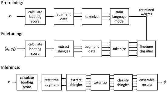
Figure 1.
Overview of approach to composer style classification of sheet music images. The input x is a raw sheet music image, and the label y indicates the composer.
2.1. Pretraining
The first stage is to pretrain the model using self-supervised language modeling. Given a set of unlabeled sheet music images, the output of the pretraining stage is a trained language model. The pretraining consists of four steps, as shown at the top of Figure 1.
The first step of pretraining is to convert each sheet music image into a bootleg score representation. The bootleg score [41] is a mid-level feature representation that encodes the sequence and positions of filled noteheads in sheet music. It was originally proposed for a sheet image-MIDI retrieval task, but has been successfully applied to other tasks such as sheet music identification [2] and audio-sheet image synchronization [43]. The bootleg score itself is a binary matrix, where 62 indicates the total number of possible staff line positions in both the left- and right-hand staves and N indicates the total number of grouped note events after collapsing simultaneous note onsets (e.g., a chord containing four notes would constitute a single grouped note event). Figure 2 shows a short excerpt of sheet music and its corresponding bootleg score which contains grouped note events. The bootleg score is computed by detecting three types of musical objects in the sheet music: staff lines, bar lines, and filled noteheads. Because these objects all have simple geometric shapes (i.e., straight lines and circles), they can be detected reliably and efficiently using classical computer vision techniques such as erosion, dilation, and blob detection. The feature extraction has no trainable weights and only about 30 hyperparameters, so it is very robust to overfitting. Indeed, the feature representation has been successfully used with very different types of data, including synthetic sheet music, scanned sheet music, and cell phone pictures of physical sheet music. For more details on the bootleg score feature representation, the reader is referred to [41].

Figure 2.
A short excerpt of sheet music and its corresponding bootleg score. Filled noteheads in the sheet music are identified and encoded as a sequence of binary columns in the bootleg score representation. The staff lines in the bootleg score are shown as a visual aid, but are not present in the actual representation.
The second step in pretraining is to augment the data by pitch shifting. One interesting characteristic about the bootleg score representation is that key transpositions correspond to shifts in the feature representation. Therefore, one easy way to augment the data is to consider shifted versions of each bootleg score up to a maximum of shifts. For example, when , this augmentation strategy will result in five times more data: the original data plus versions with shifts of , , , and . When pitch shifting causes a notehead to “fall off” the bootleg score canvas (e.g., a notehead near the top of the left-hand staff gets shifted up beyond the staff’s range), the notehead is simply eliminated. In our experiments, we considered values of K up to 3.
The third step in pretraining is to tokenize each bootleg score into a sequence of words or subwords. This is done in one of two ways, depending on the underlying language model. For word-based language models (e.g., AWD-LSTM [44]), each column of the bootleg score is treated as a single word. In practice, this can be done easily by simply representing each column of 62 bits as a single 64-bit integer. Words that occur fewer than three times in the data are mapped to a special unknown token <UNK>. For subword-based language models (e.g., GPT-2 [36], RoBERTa [45]), each column of the bootleg score is represented as a sequence of 8 bytes, where each byte constitutes a single character. The list of unique characters forms the initial vocabulary set. We then apply a byte pair encoding (BPE) algorithm [46] to iteratively merge the most frequently occurring pairs of adjacent vocabulary items until we reach a desired subword vocabulary size. In our experiments, we use a vocabulary size of 30,000 subwords. The (trained) byte pair encoder can be used to transform a sequence of 8-bit characters into a sequence of subwords. This type of subword tokenization is commonly used in modern language models. At the end of this third step, each bootleg score is represented as a sequence of word or subword units.
The fourth step in pretraining is to train a language model on the sequence of words or subwords. In this work, we consider three different language models: AWD-LSTM [44], GPT-2 [36], and RoBERTa [45]. The AWD-LSTM is a 3-layer LSTM model that incorporates several different types of dropout throughout the model. The model is trained to predict the next word at each time step. The GPT-2 model is a 6-layer Transformer decoder model that is trained to predict the next subword at each time step. The subword units are fed into an embedding layer, combined with positional word embeddings, and then fed to a sequence of six Transformer decoder layers. Though larger versions of GPT-2 have been studied [36], we only consider a modestly sized GPT-2 architecture for computational and practical reasons. The RoBERTa model is a 6-layer Transformer encoder model that is trained on a masked language modeling task. During training, a certain fraction of subwords in the input are randomly masked, and the model is trained to predict the identity of the masked tokens. Note that, unlike the transformer decoder model, the encoder model uses information from an entire sequence and is not limited only to information in the past. RoBERTa is an optimized version of BERT [37], which has been the basis of many recent language models (e.g., [47,48,49]). For both GPT-2 and RoBERTa, the context window of the language model was set very conservatively (1024) to ensure that all sequences of interest would be considered in their entirety during the classification stage (i.e., no inputs would be shortened due to being too long). Note that, though we focus only on these three language model architectures in this work, our general approach would be compatible with any model that can process sequential data (e.g., GPT-3 [38], temporal convolutional networks [50], quasi-recurrent neural networks [51]).
2.2. Finetuning
The second stage is to finetune the pretrained classifier on labeled data. The finetuning process consists of five steps, as shown in the middle row of Figure 1.
The first step is to compute bootleg score features on the labeled sheet music images. Because each piece (i.e., PDF) contains multiple pages, we concatenated the bootleg scores from all labeled pages in the PDF into a single, global bootleg score. At the end of this first step, we have a set of M bootleg scores of variable length, where M corresponds to the number of pieces in the labeled dataset.
The second step is to randomly select fixed-length fragments from the bootleg scores. This can be interpreted as a data augmentation strategy analogous to taking random crops from images. This approach has two significant benefits. First, it allows us to train on a much larger set of data. Rather than being limited to the number of actual pages in the labeled data set, we can aggressively sample the data to generate a much larger set of unique training samples. Second, it allows us to construct a balanced dataset. By sampling the same number of fragments from each classification category, we can avoid many of the problems and challenges of imbalanced datasets [52]. In our experiments, we considered fragments of length 64, 128, and 256. Figure 3 shows several example fragments from different composers.
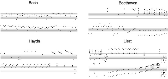
Figure 3.
Several examples of fixed-length bootleg score fragments.
The third step is to augment the labeled fragment data through pitch shifting. Similar to before, we consider multiple shifted versions of each fragment up to shifts. This is an additional data augmentation that increases the number of labeled training samples by a factor of .
The fourth step is to tokenize each fragment into a sequence of words or subwords. The tokenization is done in the same manner as described in Section 2.1. For word-based models, each fragment will produce sequences of the same length. For subword-based model, each fragment will produce sequences of (slightly) different lengths based on the output of the byte pair encoder. At the end of the fourth step, we have a set of labeled data that has been augmented, where each data sample is a sequence of words or subwords.
The fifth step is to finetune the pretrained classifier. We take the pretrained language model, add a classification head on top, and train the classification model on the labeled data using standard cross-entropy loss. Because the language model weights have been pretrained, the only part of the model that needs to be trained from scratch is the classification head. For the AWD-LSTM model, the classification head consists of the following: (a) it performs max pooling along the sequence dimension of the outputs of the last LSTM layer, (b) it performs average pooling along the sequence dimension of the outputs of the last LSTM layer, (c) it concatenates the results of these two pooling operations, and (d) passes the result to two dense layers with batch normalization and dropout. For the GPT-2 model, the classification head is a simple linear layer applied to the output of the last Transformer layer at the last time step. For the RoBERTa model, the classification head is a single linear layer applied to the output of the last Transformer layer at the first time step, which corresponds to the special beginning-of-sequence token <s>. This is the approach recommended in the original paper.
The finetuning is done using the methods described in [33]. First, we use a learning rate range finding test [53] to determine a suitable learning rate. Next, the classifier is trained with the pretrained language model weights frozen, so that only the weights in the classification head are updated. This prevents catastrophic forgetting in the pretrained weights. As training reaches convergence, we unfreeze more and more layers of the model backbone using discriminative learning rates, in which earlier layers use smaller learning rates than later layers. All training is done using 1 cycle training [54], in which the global learning rate is varied cyclically. These methods were found to be effective for finetuning text classifiers in [33].
At the end of this stage, we have a finetuned classifier that can classify fixed-length fragments of bootleg score data.
2.3. Inference
The third stage is to classify unseen sheet music images using our finetuned classifier. This inference consists of six steps, as shown at the bottom of Figure 1. The first step is to compute bootleg score features on the sheet music image. This is done in the same manner as described in Section 2.1. The second step is to perform test time augmentation using pitch shifting. Multiple shifted versions of the bootleg score are generated up to shifts, where L is a hyperparameter. Each of these bootleg scores is processed by the model (as described in the remainder of this paragraph), and we average the predictions to generate an ensembled prediction. The third step is to extract fixed-length fragments from the bootleg score. Because the bootleg score for a single page of sheet music will have variable length, we extract a sequence of fixed-length fragments with 50% overlap. Each fragment is processed independently by the model and the results are averaged. Note that the second and third steps are both forms of test time augmentation, which is a widely used technique in computer vision (e.g., taking multiple crops from a test image and averaging the results) [55,56]. The fourth step is to tokenize each fixed-length fragment into a sequence of words or subwords. This is done using the same tokenization process described in Section 2.1. The fifth step is to process each fragment’s sequence of words or subwords with the finetuned classifier. The sixth step is to compute the average of the pre-softmax outputs from all fragments across all pitch-shifted versions to produce a single ensembled pre-softmax distribution for the entire page of sheet music.
3. Results
In this section we describe our experimental setup and present our results on the composer style classification task.
3.1. Experimental Setup
There are two sets of data that we use in our experiments: an extremely large unlabeled dataset and a smaller, carefully curated labeled dataset.
The unlabeled dataset consists of all solo piano sheet music images in IMSLP. We used the instrument metadata to identify all solo piano pieces. Because popular pieces often have many different sheet music editions, we selected one sheet music version (i.e., PDF) per piece to avoid overrepresentation of a small number of popular pieces. We computed bootleg score features for all sheet music images and discarded any pages containing less than a threshold number of bootleg score features. This threshold was selected as a simple heuristic to remove non-music pages such as title page, forematerial, and other filler pages. The resulting set of data contains 29,310 PDFs, 255,539 pages, and 48.5 million bootleg score features. We will refer to this unlabeled dataset as the IMSLP data. 90% of the unlabeled data was used for language model training and 10% for validation.
The labeled dataset is a carefully curated subset of the IMSLP data. We first identified nine composers who had a substantial amount of piano sheet music. (The limit of 9 was chosen to avoid extreme imbalance of data among composers.) We constructed an exhaustive list of all solo piano pieces composed by these nine composers, and then selected one sheet music version per piece. We then manually identified filler pages in the resulting set of PDFs to ensure that every labeled image contains actual sheet music. The resulting set of data contains 787 PDFs, 7151 pages, and 1.47 million bootleg score features. Table 1 shows a breakdown of the labeled dataset by composer. The labeled data was split by piece into training, validation, and test sets. In total, there are 4347 training, 1500 validation, and 1304 test images. This dataset will be referred to as the full-page data.

Table 1.
Overview of the labeled (full-page) dataset used for classifier finetuning.
The full-page data was further preprocessed into fragments as described in Section 2.2. In our experiments, we considered three different fragment sizes: 64, 128, and 256. We sampled the same number of fragments from each composer to ensure balanced classes. For fragment size of 64, we sampled a total of 32,400, 10,800, and 10,800 fragments across all composers for training, validation, and test, respectively. For fragment size of 128, we sampled 16,200, 5400, and 5400 fragments across all composers for training, validation, and test. For fragment size of 256, we sampled 8100, 2700, and 2700 fragments for training, validation, and test. This sampling strategy ensures the same “coverage” of the data regardless of the fragment size. These datasets will be referred to as the fragment data.
3.2. Fragment Classification Results
We compare the performance of four different models: AWD-LSTM, GPT-2, RoBERTa, and a baseline CNN model. The CNN model follows the approach described by [24] for a composer classification task using **kern scores. Their approach is to feed a piano roll-like representation into two convolutional layers, perform average pooling of the activations along the sequence dimension, and then apply a final linear classification layer. This CNN model can be interpreted as the state-of-the-art approach as of 2019.
For each of the four models, we compare the performance under three different pretraining conditions. The first condition is no pretraining, in which the model is trained from scratch on the labeled fragment data. The second condition is target pretraining, in which a language model is first pretrained on the labeled (full-page) dataset, and then the pretrained classifier is finetuned on the labeled fragment data. The third condition is IMSLP pretraining, which consists of three steps: (1) training a language model on the full IMSLP dataset, (2) finetuning the language model on the labeled dataset, and (3) finetuning the pretrained classifier on the labeled fragment data. The third condition corresponds to the ULMFit [33] method. Comparing the performance under these three conditions will allow us to measure how much pretraining improves the performance of the classifier.
Figure 4 shows the performance of all models on the fragment classification task. While our original goal is to classify full-page images, the performance on the test fragment data is useful because the dataset is balanced and more reliable due to its much larger size (i.e., number of samples). The three groups in the figure correspond to fragment sizes of 64 (left), 128 (middle), and 256 (right). For a given fragment size, the bars indicate the classification accuracy of all models, where different colors correspond to different pretraining conditions. Note that the CNN model only has results for the no pretraining condition, since it is not a language model. The bars indicate the performance of each model with training data augmentation and test time augmentation . These settings were found to be best for the best-performing model (see Section 4.1) and were applied to all models in Figure 4 for fair comparison. The performance with no data augmentation (, ) is also overlaid as black rectangles for comparison.

Figure 4.
Results on the fragment classification task. For each model architecture, the green (leftmost), blue (center), and red (rightmost) bars show the performance with no pretraining, target pretraining, and full IMSLP pretraining, respectively. Colored bars indicate performance with both training and test time data augmentation (, ), and black rectangles indicate performance without augmentation (, ).
There are four things to notice about Figure 4. First, pretraining makes a big difference. For all language model architectures, we see a large and consistent improvement from pretraining. For example, for the RoBERTa model with fragment size 64, the accuracy improves from 50.9% to 72.0% to 81.2% across the three pretraining conditions. Second, the augmentation strategies make a big difference. Regardless of model architecture or pretraining condition, we see a very large improvement in classification performance. For example, the AWD-LSTM model with IMSLP pretraining and fragment size 64 improves from 53.0% to 75.9% when incorporating data augmentation. The effect of the training and test-time augmentation will be studied in more depth in Section 4.1. Third, the Transformer-based models outperform the LSTM and CNN models. The best model (GPT-2 with IMSLP pretraining) achieves a classification accuracy of 90.2% for fragment size 256. Fourth, the classification performance improves as fragment size increases. This is to be expected, since having more context information should improve classification performance.
3.3. Full-Page Classification Results
Figure 5 shows the performance of all models on the full-page classification task. This is the original task that we set out to solve. Note that the y-axis is now macro F1, since accuracy is only an appropriate metric when the dataset is approximately balanced. These results should be interpreted with caution, keeping in mind that the test (full-page) dataset is relatively small in size (1304 images) and also has class imbalance.
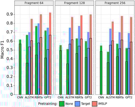
Figure 5.
Results on the full-page classification task. For each model architecture, the green (leftmost), blue (center), and red (rightmost) bars show the performance with no pretraining, target pretraining, and full IMSLP pretraining, respectively. Colored bars indicate performance with both training and test time data augmentation (, ), and black rectangles indicate performance without augmentation (, ).
There are a few things to point out about Figure 5. Most of the trends observed in the fragment classification task hold true for the full-page classification task: pretraining helps significantly, data augmentation helps significantly, and the Transformer-based models perform best. However, one trend is reversed for the full-page classification task: longer fragments sizes yield worse full-page classification performance. This suggests a mismatch between the fragment dataset and the fragments in the full-page data. Indeed, when we investigated this issue more closely, we found that many sheet music images had less than 128 or 256 bootleg score features on the whole page. This means that the fragment datasets with sizes 128 and 256 are biased towards sheet music containing a very large number of note events on a single page, and are not representative of single pages of sheet music. For this reason, the fragment classification with length 64 is most effective for the full-page classification task.
4. Discussion
In this section we perform four additional analyses to gain deeper insight and intuition into the best-performing model: GPT-2 with IMSLP pretraining and fragment size 64.
4.1. Effect of Data Augmentation
The first analysis is to characterize the effect of the training and test time augmentation strategies. Recall that the bootleg scores are shifted by up to shifts during training, and that shifted versions of each query up to shifts are ensembled at test time. Figure 6 shows the fragment classification performance of the GPT-2 model with IMSLP pretraining across a range of K and L values. Figure 7 shows the performance of the same models on the full-page classification task.
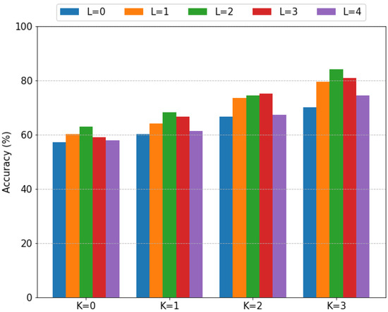
Figure 6.
Effect of data augmentation on fragment classification performance (fragment length 64). K specifies the amount of training data augmentation and L specifies the amount of test time data augmentation. Within each grouping, the bars correspond to values of L ranging from 0 (leftmost) to 4 (rightmost).
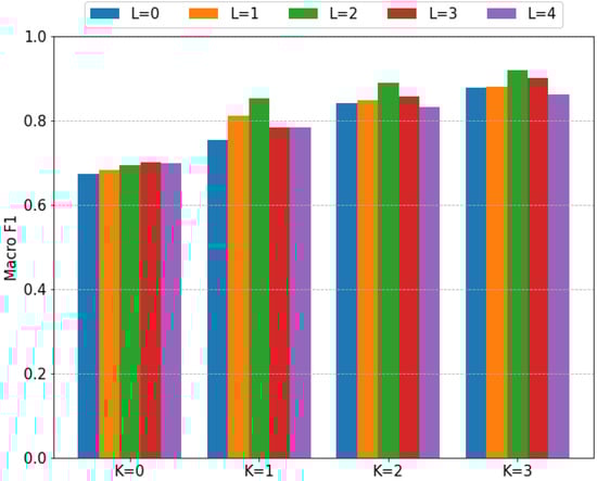
Figure 7.
Effect of data augmentation on full-page classification performance (fragment length 64). K specifies the amount of training data augmentation and L specifies the amount of test time data augmentation. Within each grouping, the bars correspond to values of L ranging from 0 (leftmost) to 4 (rightmost).
There are two notable things to point out in Figure 6 and Figure 7. First, higher values of K lead to significant increases in model performance. For example, the performance of the GPT-2 model with increases from to macro F1 as K increases from 0 to 3. Based on the trends shown in these figures, we would expect even better performance for values of K greater than 3. We only considered values up to 3 due to the extremely long training times. Second, test time augmentation helps significantly but only when used in moderation. For most values of K, the optimal value of L is 2 or 3. As L continues to increase, the performance begins to degrade. Combining both training and test time augmentation, we see extremely large improvements in model performance: the fragment classification accuracy increases from 57.3% (, ) to 84.2% (, ), and the full-page classification performance increases from macro F1 (, ) to macro F1 (, ).
The takeaway from our first analysis is clear: training and test time augmentation improve the model performance significantly and should always be used.
4.2. Single Hand Models
The second analysis is to quantify how important the right hand and left hand are in classification. The bootleg score contains 62 distinct staff line positions, of which 34 come from the right hand staff (E3 to C8) and 28 come from the left hand staff (A0 to G4). To study the importance of each hand, we trained two single-hand models: a right hand model in which any notes in the left hand staff are zeroed out, and a left hand model in which any notes in the right hand staff are zeroed out. We trained a BPE for each hand separately, pretrained the GPT-2 language model on the appropriately masked IMSLP data, finetuned the classifier on the masked training fragment data, and then evaluated the performance on the masked test fragment data.
Figure 8 compares the results of the right hand and left hand models against the full model containing both hands. We see that, regardless of the pretraining condition, the right hand model outperforms the left hand model by a large margin. This matches our intuition, since the right hand tends to contain the melody and is more distinctive than the left hand accompaniment part. We also see a big gap in performance between the single hand models and the full model containing both hands. This suggests that a lot of the information needed for classification comes from the polyphonic, harmonic component of the music. If our approach were applied to monophonic music, for example, we would expect performance to be worse than the right hand model.
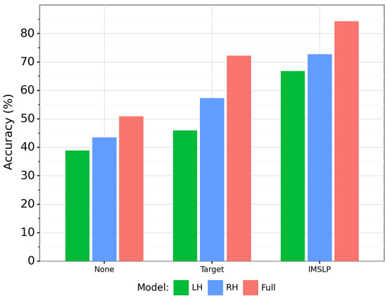
Figure 8.
Comparison of GPT-2 model on fragment classification using left hand information only (green bars, leftmost in each group), right hand information only (blue bars, center in each group), and information from both hands (red bars, rightmost in each group). The three groups of bars correspond to different pretraining conditions.
4.3. t-SNE
The third analysis is to visualize a t-SNE plot [57] of selected bootleg score features. Specifically, we extracted the learned embeddings for all bootleg score columns containing a single notehead, and then visualized them in a t-SNE plot. Because byte pair encoding (in the subword-based language models) makes it difficult to examine a single bootleg score column, we focus on the word-based AWD-LSTM model (trained on fragments of length 64) for this analysis. Note that our model does not explicitly encode any musical domain knowledge, so any relationships that we discover are an indication that the model has learned semantically meaningful information from the data.
Figure 9 shows the t-SNE plot for the embeddings of single notehead bootleg score features. We can see two distinct clusters: one cluster containing noteheads in the right hand staff (lower left), and another cluster containing noteheads in the left hand staff (upper right). Within each cluster, we see that noteheads that appear close to one another in the sheet music are close to one another in the t-SNE plot. This results in an approximately linear progression (with lots of zigzags) from low noteheads to high noteheads. This provides strong evidence that the model is able to learn semantically meaningful relationships between different bootleg score features, even though each word is considered a distinct entity.
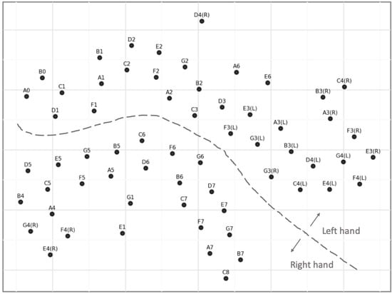
Figure 9.
A t-SNE plot of the AWD-LSTM embeddings for bootleg score features containing a single notehead. Note that some notehead positions in the middle register may appear in either the left-hand staff or right-hand staff. With only a few exceptions, the notes cluster by left hand (upper right) and right hand (lower left) staves.
4.4. Unseen Composer Classification
The fourth analysis is to determine if the models learn a more generalizable notion of style that extends beyond the nine composers in the classification task. To answer this question, we perform the following experiment. First, we randomly sample C composers from the full IMSLP dataset, making sure to exclude the nine composers in the training data. Next, we assemble all sheet music images for solo piano works composed by these C composers. For each page of sheet music in this newly constructed data set, we (a) pass the sheet music image through our full-page classification model, (b) take the penultimate layer activations in the model as a feature representation of the page, (c) calculate the average Euclidian distance to the nearest neighbors (each corresponding to a single page of sheet music) for each of the C composers, and (d) rank the C composers according to their KNN distance scores. For step (c), we exclude all other pages from the same piece, so that the similarity to the true matching composer must be computed against other pieces written by the composer. Finally, we repeat the above experiment times and report the mean reciprocal rank of all predictions.
Figure 10 shows the results of these experiments. We evaluate all four model architectures with fragment size 64 (with data augmentation and IMSLP pretraining), along with a random guessing model as a reference. The figure compares the results of all five models for values of C ranging from 10 to 200. We can see that all four trained models perform much better than random guessing, and that the GPT-2 model continues to perform the best. This provides evidence that the models are learning a notion of compositional style that generalizes beyond the nine composers in the labeled dataset. The trained models can thus be used as a feature extractor to project a page of sheet music into this compositional style feature space.

Figure 10.
Comparison of models on a ranking task involving unseen composers. C composers are randomly selected from IMSLP (excluding the original 9 composers in the labeled dataset), each page of piano sheet music for these C composers is considered as a query, and the KNN distance (excluding pages from the same piece) is used to rank the C composers. From left to right, the bars in each group correspond to random guessing, CNN, AWD-LSTM, RoBERTa, and GPT-2 models. Each bar shows the average of 10 such experiments.
5. Conclusions
We have proposed an approach to the composer style classification task based on raw sheet music images. Our approach converts the sheet music images to a bootleg score representation, represents the bootleg score features as sequences of words, and then treats the problem as a text classification task. Compared to previous work, our approach is novel in that it utilizes self-supervised pretraining on unlabeled data, which allows for effective classifiers to be trained even with limited amounts of labeled data. We perform extensive experiments on a range of modern language model architectures, and we show that pretraining substantially improves classification performance and that Transformer-based architectures perform best. We also introduce two data augmentation strategies and conduct various analyses to gain deeper intuition into the model. Future work includes exploring additional data augmentation and regularization strategies, as well as applying this approach to non-piano sheet music.
Author Contributions
Conceptualization, T.T.; Investigation, D.Y. and K.J.; Software, D.Y. and K.J.; Supervision, T.T.; Writing—original draft, T.T.; Writing—review & editing, D.Y. and K.J. All authors have read and agreed to the published version of the manuscript.
Funding
This research was made possible through the Brian Butler ‘89 HMC Faculty Enhancement Fund. This work used the Extreme Science and Engineering Discovery Environment (XSEDE), which is supported by National Science Foundation grant number ACI-1548562. Large-scale computations on IMSLP data were performed with XSEDE Bridges at the Pittsburgh Supercomputing Center through allocation TG-IRI190019.
Data Availability Statement
Code and data for replicating the results in this article can be found at https://github.com/HMC-MIR/ComposerID.
Conflicts of Interest
The authors declare no conflict of interest. The funders had no role in the design of the study; in the collection, analyses, or interpretation of data; in the writing of the manuscript, or in the decision to publish the results.
Abbreviations
The following abbreviations are used in this manuscript:
| OMR | Optical Music Recognition |
| IMSLP | International Music Score Library Project |
| KNN | K Nearest Neighbors |
| SVM | Support Vector Machine |
| CNN | Convolutional Neural Network |
| MIDI | Musical Instrument Digital Interface |
| NLP | Natural Language Processing |
| ULMFit | Universal Language Model Fine Tuning |
| LSTM | Long Short-Term Memory |
| GPT-2 | Generative Pretraining |
| BERT | Bidirectional Encoder Representations from Transformers |
| RoBERTa | A Robustly Optimized BERT Pretraining Approach |
| AWD-LSTM | Average Stochastic Gradient Descent Weight-Dropped LSTM |
| Portable Document Format | |
| BPE | Byte Pair Encoder |
| t-SNE | t-Distributed Stochastic Neighbor Embedding |
| MRR | Mean Reciprocal Rank |
References
- Calvo-Zaragoza, J.; Hajič, J., Jr.; Pacha, A. Understanding Optical Music Recognition. ACM Comput. Surv. (CSUR) 2020, 53, 1–35. [Google Scholar] [CrossRef]
- Yang, D.; Tsai, T. Camera-Based Piano Sheet Music Identification. In Proceedings of the International Society for Music Information Retrieval Conference (ISMIR), Montréal, QC, Canada, 11–15 October 2020; pp. 481–488. [Google Scholar]
- Dorfer, M.; Hajič, J.; Arzt, A.; Frostel, H.; Widmer, G. Learning Audio-Sheet Music Correspondences for Cross-Modal Retrieval and Piece Identification. Trans. Int. Soc. Music Inf. Retr. 2018, 1, 22–33. [Google Scholar] [CrossRef]
- Henkel, F.; Kelz, R.; Widmer, G. Learning to Read and Follow Music in Complete Score Sheet Images. In Proceedings of the International Society for Music Information Retrieval Conference (ISMIR), Montréal, QC, Canada, 11–15 October 2020; pp. 780–787. [Google Scholar]
- Tsai, T. Towards Linking the Lakh and IMSLP Datasets. In Proceedings of the IEEE International Conference on Acoustics, Speech, and Signal Processing (ICASSP), Barcelona, Spain, 4–8 May 2020; pp. 546–550. [Google Scholar]
- Anan, Y.; Hatano, K.; Bannai, H.; Takeda, M.; Satoh, K. Polyphonic Music Classification on Symbolic Data Using Dissimilarity Functions. In Proceedings of the International Society for Music Information Retrieval Conference (ISMIR), Porto, Portugal, 8–12 October 2012; pp. 229–234. [Google Scholar]
- Kaliakatsos-Papakostas, M.A.; Epitropakis, M.G.; Vrahatis, M.N. Musical Composer Identification Through Probabilistic and Feedforward Neural Networks. In Proceedings of the European Conference on the Applications of Evolutionary Computation, Istanbul, Turkey, 7–9 April 2010; pp. 411–420. [Google Scholar]
- Herlands, W.; Der, R.; Greenberg, Y.; Levin, S. A Machine Learning Approach to Musically Meaningful Homogeneous Style Classification. In Proceedings of the Twenty-Eighth AAAI Conference on Artificial Intelligence, Québec City, QC, Canada, 27–31 July 2014. [Google Scholar]
- Backer, E.; van Kranenburg, P. On Musical Stylometry—A Pattern Recognition Approach. Pattern Recognit. Lett. 2005, 26, 299–309. [Google Scholar] [CrossRef]
- Kempfert, K.C.; Wong, S.W. Where Does Haydn End And Mozart Begin? Composer Classification Of String Quartets. arXiv 2018, arXiv:1809.05075. [Google Scholar] [CrossRef]
- Mearns, L.; Tidhar, D.; Dixon, S. Characterisation of Composer Style using High-Level Musical Features. In Proceedings of the 3rd International Workshop on Machine Learning and Music, Firenze, Italy, 29 October 2010; pp. 37–40. [Google Scholar]
- Van Kranenburg, P.; Backer, E. Musical Style Recognition—A Quantitative Approach. In Handbook of Pattern Recognition and Computer Vision; World Scientific Publishing Co.: Singapore, 2005; pp. 583–600. [Google Scholar]
- Hillewaere, R.; Manderick, B.; Conklin, D. String Quartet Classification with Monophonic Models. In Proceedings of the International Society for Music Information Retrieval Conference (ISMIR), Utrecht, The Netherlands, 9–13 August 2010; pp. 537–542. [Google Scholar]
- Herremans, D.; Martens, D.; Sörensen, K. Composer Classification Models for Music-Theory Building. In Computational Music Analysis; Springer: Berlin, Germany, 2016; pp. 369–392. [Google Scholar]
- McKay, C.; Fujinaga, I. jSymbolic: A Feature Extractor for MIDI Files. In Proceedings of the International Computer Music Conference, New Orleans, LA, USA, 6–11 November 2006. [Google Scholar]
- Brinkman, A.; Shanahan, D.; Sapp, C. Musical Stylometry, Machine Learning and Attribution Studies: A Semi-Supervised Approach to the Works of Josquin. In Proceedings of the Biennial International Conference on Music Perception and Cognition, San Francisco, CA, USA, 5–9 July 2016; pp. 91–97. [Google Scholar]
- Sadeghian, P.; Wilson, C.; Goeddel, S.; Olmsted, A. Classification of Music by Composer Using Fuzzy Min-Max Neural Networks. In Proceedings of the 12th International Conference for Internet Technology and Secured Transactions (ICITST), Cambridge, UK, 11–14 December 2017; pp. 189–192. [Google Scholar]
- Hontanilla, M.; Pérez-Sancho, C.; Inesta, J.M. Modeling Musical Style with Language Models for Composer Recognition. In Proceedings of the Iberian Conference on Pattern Recognition and Image Analysis, Madeira, Portugal, 5–7 June 2013; pp. 740–748. [Google Scholar]
- Wołkowicz, J.; Kešelj, V. Evaluation of N-gram-based Classification Approaches on Classical Music Corpora. In Proceedings of the International Conference on Mathematics and Computation in Music, Montreal, QC, Canada, 12–14 June 2013; pp. 213–225. [Google Scholar]
- Wołkowicz, J.; Kulka, Z.; Kešelj, V. N-gram-based Approach to Composer Recognition. Arch. Acoust. 2008, 33, 43–55. [Google Scholar]
- Kaliakatsos-Papakostas, M.A.; Epitropakis, M.G.; Vrahatis, M.N. Weighted Markov Chain Model for Musical Composer Identification. In Proceedings of the European Conference on the Applications of Evolutionary Computation, Torino, Italy, 27–29 April 2011; pp. 334–343. [Google Scholar]
- Pollastri, E.; Simoncelli, G. Classification of Melodies by Composer with Hidden Markov Models. In Proceedings of the First International Conference on WEB Delivering of Music, Florence, Italy, 23–24 November 2001; pp. 88–95. [Google Scholar]
- Buzzanca, G. A Supervised Learning Approach to Musical Style Recognition. In Proceedings of the International Conference on Music and Artificial Intelligence (ICMAI), Edinburgh, UK, 12–14 September 2002; Volume 2002, p. 167. [Google Scholar]
- Verma, H.; Thickstun, J. Convolutional Composer Classification. In Proceedings of the International Society for Music Information Retrieval Conference (ISMIR), Delft, The Netherlands, 4–8 November 2019; pp. 549–556. [Google Scholar]
- Velarde, G.; Chacón, C.C.; Meredith, D.; Weyde, T.; Grachten, M. Convolution-based Classification of Audio and Symbolic Representations of Music. J. New Music Res. 2018, 47, 191–205. [Google Scholar] [CrossRef]
- Velarde, G.; Weyde, T.; Chacón, C.E.C.; Meredith, D.; Grachten, M. Composer Recognition Based on 2D-Filtered Piano-Rolls. In Proceedings of the International Society for Music Information Retrieval Conference (ISMIR), New York, NY, USA, 7–11 August 2016; pp. 115–121. [Google Scholar]
- Good, M.; Actor, G. Using MusicXML for File Interchange. In Proceedings of the Third International Conference on WEB Delivering of Music, Leeds, UK, 15–17 September 2003; p. 153. [Google Scholar]
- Huron, D. Humdrum and Kern: Selective Feature Encoding; MIT Press: Cambridge, MA, USA, 1997. [Google Scholar]
- Hankinson, A.; Roland, P.; Fujinaga, I. The Music Encoding Initiative as a Document-Encoding Framework. In Proceedings of the International Society for Music Information Retrieval Conference (ISMIR), Miami, FL, USA, 24–28 October 2011; pp. 293–298. [Google Scholar]
- Mikolov, T.; Sutskever, I.; Chen, K.; Corrado, G.S.; Dean, J. Distributed Representations of Words and Phrases and their Compositionality. Adv. Neural Inf. Process. Syst. 2013, 26, 3111–3119. [Google Scholar]
- Mikolov, T.; Chen, K.; Corrado, G.; Dean, J. Efficient Estimation of Word Representations in Vector Space. arXiv 2013, arXiv:1301.3781. [Google Scholar]
- Pennington, J.; Socher, R.; Manning, C.D. GloVe: Global Vectors for Word Representation. In Proceedings of the Conference on Empirical Methods in Natural Language Processing (EMNLP), Doha, Qatar, 25–29 October 2014; pp. 1532–1543. [Google Scholar]
- Howard, J.; Ruder, S. Universal Language Model Fine-tuning for Text Classification. In Proceedings of the 56th Annual Meeting of the Association for Computational Linguistics, Melbourne, Australia, 15–20 July 2018; pp. 328–339. [Google Scholar]
- Dai, A.M.; Le, Q.V. Semi-Supervised Sequence Learning. Adv. Neural Inf. Process. Syst. 2015, 28, 3079–3087. [Google Scholar]
- Vaswani, A.; Shazeer, N.; Parmar, N.; Uszkoreit, J.; Jones, L.; Gomez, A.N.; Kaiser, Ł.; Polosukhin, I. Attention Is All You Need. In Proceedings of the Advances in Neural Information Processing Systems, Long Beach, CA, USA, December 2017; pp. 5998–6008. [Google Scholar]
- Radford, A.; Wu, J.; Child, R.; Luan, D.; Amodei, D.; Sutskever, I. Language Models are Unsupervised Multitask Learners. OpenAI Blog 2019, 1, 9. [Google Scholar]
- Devlin, J.; Chang, M.W.; Lee, K.; Toutanova, K. BERT: Pre-training of Deep Bidirectional Transformers for Language Understanding. arXiv 2018, arXiv:1810.04805. [Google Scholar]
- Brown, T.B.; Mann, B.; Ryder, N.; Subbiah, M.; Kaplan, J.; Dhariwal, P.; Neelakantan, A.; Shyam, P.; Sastry, G.; Askell, A.; et al. Language Models are Few-Shot Learners. arXiv 2020, arXiv:2005.14165. [Google Scholar]
- Dai, Z.; Yang, Z.; Yang, Y.; Carbonell, J.G.; Le, Q.; Salakhutdinov, R. Transformer-XL: Attentive Language Models Beyond a Fixed-Length Context. In Proceedings of the 57th Annual Meeting of the Association for Computational Linguistics, Florence, Italy, 28 July–2 August 2019; pp. 2978–2988. [Google Scholar]
- Yang, Z.; Dai, Z.; Yang, Y.; Carbonell, J.; Salakhutdinov, R.R.; Le, Q.V. XLNet: Generalized Autoregressive Pretraining for Language Understanding. arXiv 2019, arXiv:1906.08237. [Google Scholar]
- Yang, D.; Tanprasert, T.; Jenrungrot, T.; Shan, M.; Tsai, T. MIDI Passage Retrieval Using Cell Phone Pictures of Sheet Music. In Proceedings of the International Society for Music Information Retrieval Conference (ISMIR), Delft, The Netherlands, 4–8 November 2019; pp. 916–923. [Google Scholar]
- Yang, D.; Tsai, T. Composer Style Classification of Piano Sheet Music Images Using Language Model Pretraining. In Proceedings of the International Society for Music Information Retrieval Conference (ISMIR), Montréal, QC, Canada, 11–15 October 2020; pp. 176–183. [Google Scholar]
- Shan, M.; Tsai, T. Improved Handling of Repeats and Jumps in Audio-Sheet Image Synchronization. In Proceedings of the International Society for Music Information Retrieval Conference (ISMIR), Montréal, QC, Canada, 11–15 October 2020; pp. 62–69. [Google Scholar]
- Merity, S.; Keskar, N.S.; Socher, R. Regularizing and Optimizing LSTM Language Models. arXiv 2017, arXiv:1708.02182. [Google Scholar]
- Liu, Y.; Ott, M.; Goyal, N.; Du, J.; Joshi, M.; Chen, D.; Levy, O.; Lewis, M.; Zettlemoyer, L.; Stoyanov, V. RoBERTa: A Robustly Optimized BERT Pretraining Approach. arXiv 2019, arXiv:1907.11692. [Google Scholar]
- Gage, P. A New Algorithm for Data Compression. C Users J. 1994, 12, 23–38. [Google Scholar]
- Martin, L.; Muller, B.; Suárez, P.J.O.; Dupont, Y.; Romary, L.; de la Clergerie, É.V.; Seddah, D.; Sagot, B. CamemBERT: A Tasty French Language Model. arXiv 2019, arXiv:1911.03894. [Google Scholar]
- Lan, Z.; Chen, M.; Goodman, S.; Gimpel, K.; Sharma, P.; Soricut, R. ALBERT: A Lite BERT for Self-Supervised Learning of Language Representations. arXiv 2019, arXiv:1909.11942. [Google Scholar]
- Sanh, V.; Debut, L.; Chaumond, J.; Wolf, T. DistilBERT, a Distilled Version of BERT: Smaller, Faster, Cheaper and Lighter. arXiv 2019, arXiv:1910.01108. [Google Scholar]
- Bai, S.; Kolter, J.Z.; Koltun, V. An Empirical Evaluation of Generic Convolutional and Recurrent Networks for Sequence Modeling. arXiv 2018, arXiv:1803.01271. [Google Scholar]
- Bradbury, J.; Merity, S.; Xiong, C.; Socher, R. Quasi-Recurrent Neural Networks. arXiv 2016, arXiv:1611.01576. [Google Scholar]
- Buda, M.; Maki, A.; Mazurowski, M.A. A Systematic Study of the Class Imbalance Problem in Convolutional Neural Networks. Neural Netw. 2018, 106, 249–259. [Google Scholar] [CrossRef] [PubMed]
- Smith, L.N. Cyclical Learning Rates for Training Neural Networks. In Proceedings of the 2017 IEEE Winter Conference on Applications of Computer Vision (WACV), Santa Rosa, CA, USA, 27–29 March 2017; pp. 464–472. [Google Scholar]
- Smith, L.N. A Disciplined Approach to Neural Network Hyper-parameters: Part 1–Learning Rate, Batch Size, Momentum, and Weight Decay. arXiv 2018, arXiv:1803.09820. [Google Scholar]
- Taylor, L.; Nitschke, G. Improving Deep Learning Using Generic Data Augmentation. arXiv 2017, arXiv:1708.06020. [Google Scholar]
- Calvo-Zaragoza, J.; Rico-Juan, J.R.; Gallego, A.J. Ensemble Classification from Deep Predictions with Test Data Augmentation. Soft Comput. 2020, 24, 1423–1433. [Google Scholar] [CrossRef]
- Van der Maaten, L.; Hinton, G. Visualizing Data Using t-SNE. J. Mach. Learn. Res. 2008, 9, 2579–2605. [Google Scholar]
Publisher’s Note: MDPI stays neutral with regard to jurisdictional claims in published maps and institutional affiliations. |
© 2021 by the authors. Licensee MDPI, Basel, Switzerland. This article is an open access article distributed under the terms and conditions of the Creative Commons Attribution (CC BY) license (http://creativecommons.org/licenses/by/4.0/).