Article

Pose Measurement for Unmanned Aerial Vehicle Based on Rigid Skeleton

Ministry of Education Key Laboratory of Precision Opto-Mechatronics Technology, Beihang University, Beijing 100191, China
*
Author to whom correspondence should be addressed.
Appl. Sci. 2021, 11(4), 1373; https://doi.org/10.3390/app11041373
Submission received: 30 December 2020 / Revised: 28 January 2021 / Accepted: 1 February 2021 / Published: 3 February 2021
(This article belongs to the Collection Machine Learning in Computer Engineering Applications)

Abstract

:
Pose measurement is a necessary technology for UAV navigation. Accurate pose measurement is the most important guarantee for a UAV stable flight. UAV pose measurement methods mostly use image matching with aircraft models or 2D points corresponding with 3D points. These methods will lead to pose measurement errors due to inaccurate contour and key feature point extraction. In order to solve these problems, a pose measurement method based on the structural characteristics of aircraft rigid skeleton is proposed in this paper. The depth information is introduced to guide and label the 2D feature points to eliminate the feature mismatch and segment the region. The space points obtained from the marked feature points fit the space linear equation of the rigid skeleton, and the UAV attitude is calculated by combining with the geometric model. This method does not need cooperative identification of the aircraft model, and can stably measure the position and attitude of short-range UAV in various environments. The effectiveness and reliability of the proposed method are verified by experiments on a visual simulation platform. The method proposed can prevent aircraft collision and ensure the safety of UAV navigation in autonomous refueling or formation flight.

1. Introduction

UAVs are unmanned aircraft operated by radio remote control equipment and self-provided program control devices. They are widely used in aerial photography, agriculture, express transportation, disaster relief, surveying and mapping, news reporting, disaster relief, and other fields [1,2]. Safety and stability are the most basic and important requirements for a UAV in flight. Therefore, flight control of the UAV is a particularly essential feature. Attitude calculation is an imperative aspect of flight control [3]. The estimated attitude is released to the attitude controller [4] to ensure stable flight. Therefore, the attitude estimation is the most important guarantee of flight stability.
The measurement of aircraft position and attitude can be divided into contact measurement and non-contact measurement according to the type and position of sensors. The classification of pose measurement methods is shown in Table 1. Contact measurement is also called attitude internal measurement. The measurement sensor used in this method is attached to the aircraft and moves with it. Non-contact measurement is also called attitude external measurement. In this case, the measurement sensor is not in contact with the aircraft; instead, it is usually placed on the ground or some other platform.
Several mature sensing instruments for attitude internal measurement are available, such as global navigation satellite system (GNSS) [5,6] and inertial navigation equipment (IMU) [7,8]. These equipment can directly give high-precision attitude parameters but also present a number of obvious shortcomings in their attitude internal measurement methods, which are mainly reflected in the robustness of the measurement method and measurement accuracy will become worse under certain conditions. At the same time, the attitude measurement method is affected by factors such as calculation frequency and signal reception.
The attitude external measurement of UAV algorithms has been studied by research institutes worldwide. Some methods measure the aircraft’s pose by monocular. These methods usually need measuring equipment such as theodolite and radar. Dementhon and Davis [9] proposed SoftPOSIT, an improved algorithm of POSIT. In this algorithm, the target pose parameters can be solved iteratively when the corresponding 2D–3D points are unknown. Fishler et al. [10] proposed the N-point perspective problem, which is a PNP problem. The coordinates of N points in the target coordinate system, as well as those of the projection points on the image plane, are determined to solve the relative position and attitude relationship. Hinterstoisser et al. [11] proposed a method to generate a template according to the viewpoint and match real images to estimate the target pose. Sample templates, which include color and depth gradients, are obtained from different perspectives. The real image is matched with templates from different viewpoints, thresholds are set to obtain ideal matching results, and pose estimation is completed. The robust ICP algorithm is used to achieve 3D point set matching. Liebelt performed pose measurement based on the target contour matching method [12]. Given an initial value, iterative optimization is used to minimize deviations by calculating the deviation between the result of the target edge reprojection and the actual imaging result of the target edge. The target pose is then solved. In this method, the target edge contour need to be obtained. Luo et al. [13] adopted a line segment detector to extract line segment features, mean-shift and k-means++ approaches are applied to group line segments. This method recognized the lines corresponding to the fuselage and wing in the image to realize the structure extraction of straight wing aircraft.
Studies on attitude external measurement of UAV based on multiple cameras have been conducted. Wang Bin proposed a method to solve aircraft attitudes by using the straight-line feature information of the aircraft [14]. The rotation matrix obtained by the angle bisector method is used as an initial value, and the coplanar error formula of the linear feature space of multiple camera images is established. The spatial coplanar error of all observed straight lines is used as an objective function to solve the optimal rotation matrix iteratively. Finally, the attitude parameters are analyzed. This calculation process requires the assistance of a theodolite. Li Guorong [15] proposed a method to compare simulated images with real ones and invert the target flight attitude. The pyramid-based regional matching algorithm may be used to determine the initial value of the target’s pose parameters, after which the iterative optimization algorithm is refined and optimized on the basis of outer contour point set matching. Yuan et al. [16] proposed a combined vision technology based on a multi-camera, which combines multi-view and mono-view constraints for UAV attitude estimation. The particle filter framework combined with constraints to improve the accuracy of the algorithm. Zhang et al. [17,18] combined stereo vision with the geometric information of the object, proposed a method based on optimization to measure the position and attitude of the spacecraft and realized the attitude solution of the spacecraft with the non-cooperative target. Teng et al. [19] extracted and clustered image line features based on two widely separated cameras, combined with the common geometric constraints of straight wing aircraft to solve the aircraft attitude. The aircraft attitude measurement is realized under the condition of the large field of view and long-distance.
In practical applications, an image may be unavailable or the target may not be captured when a photometric device is used to capture images. Furthermore, algorithms that rely on 2D images usually need other information or equipment to solve the spatial pose accurately. Existing multi-eye measurement methods mainly match images with models or seek the correspondence between 2D and 3D points. These methods are negatively affected by factors such as inaccurate contour extraction, occlusion of key feature points, and incorrect matching in complex environments. Therefore, the pose measurement accuracy of these methods is low, and knowledge of the aircraft model information must be available.
In the process of flight, the skeleton structure of UAVs is rigid and almost not affected by external factors. Therefore, the attitude of UAV can be solved by the spatial straight line in the rigid skeleton.
This paper proposes a measurement method for the position and attitude of UAV based on a rigid skeleton that integrates 2D images and 3D point cloud information without requiring aircraft size or model information and then solves the problem of UAV aircraft attitude determination. The main contributions of this article are as follows:
  • A method framework based on the structural characteristics of a rigid skeleton of the aircraft is proposed to solve the position and attitude of short-range UAVs without knowledge of the aircraft model and size.
  • A key point screening method that combines 2D and 3D information is proposed for aircraft pose measurement. The method in this paper is based on a stereo vision measurement system. Depth information is combined with edge contour and corner point information to reduce the mismatch of aircraft key feature points effectively.
  • The proposed method can solve the online attitude of UAVs without identification and other auxiliary equipment, thereby effectively improving the reliability and robustness of the attitude calculation algorithm. Thus, the method can be applied to low-consumption airborne environments.
The rest of this article is organized as follows. Section 2 introduces the related knowledge and system framework. Section 3 describes the algorithm in detail. Section 4 shows the simulation experiment. The results of the entire method and comparative experiments are provided in Section 5. Finally, Section 6 summarizes the article.

2. System Framework

The attitude of an aircraft refers to the state between the three axes of the aircraft’s coordinate system and a fixed coordinate system. The flight attitude of an aircraft affects the altitude and direction of the flight. A pilot can judge the airplane’s flight attitude through the horizon when flying at low speed. However, because the attitude of the pilot body changes with the attitude of the aircraft, this type of experience-based judgment is unreliable and prone to misjudgment. Therefore, the measurement of aircraft attitude is a very important research topic in efforts to ensure the safety of aircraft navigation.

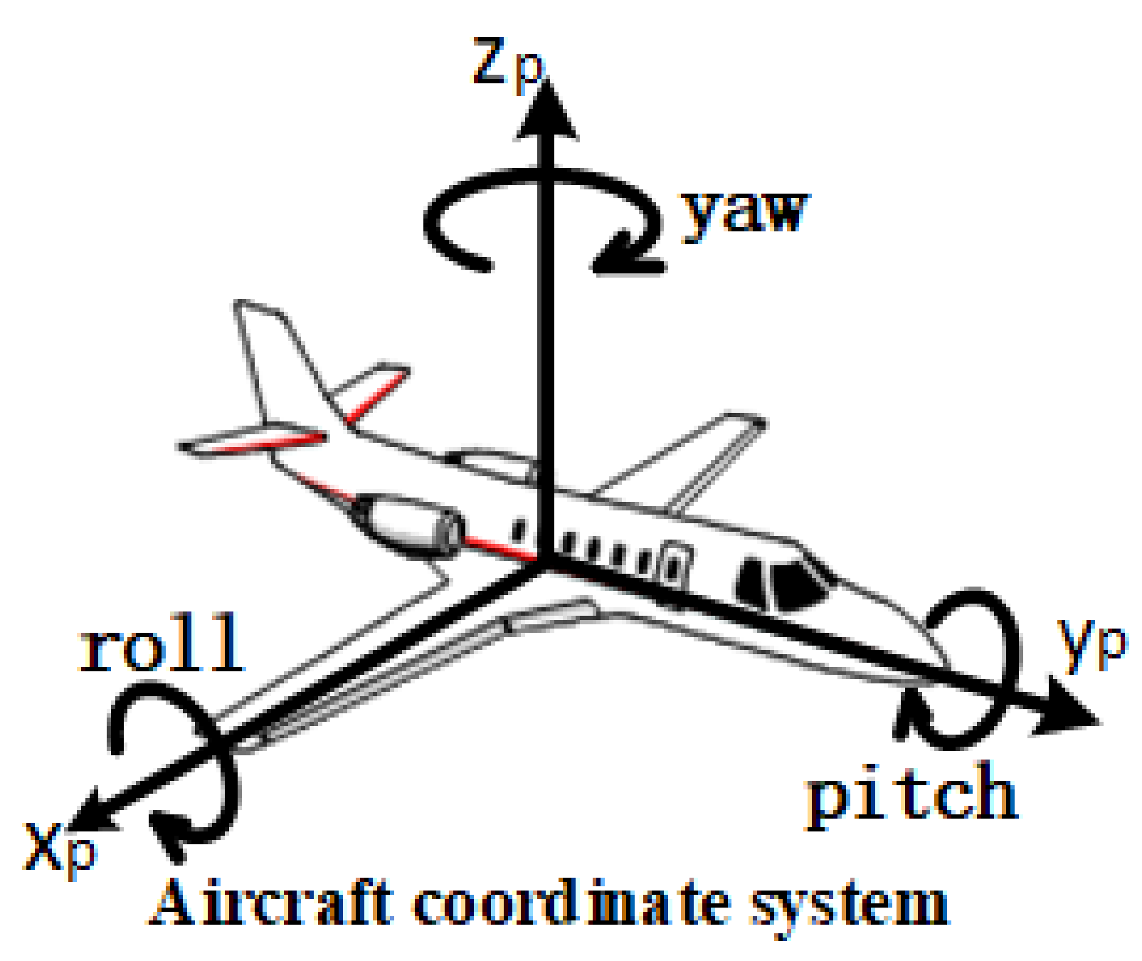
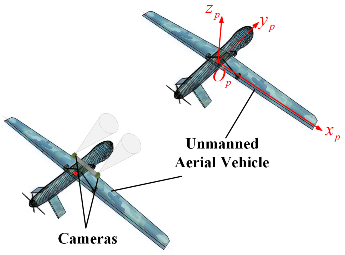
2.1. Definition of Aircraft Attitude Angle

We define the aircraft local coordinate system O p x p y p z p , as shown in Figure 1. The center point (center of mass) of the aircraft is taken as the origin of its local coordinate system O p , the direction of the wing (pointing to the right wing) is defined as the O p x p axis, the direction of the nose is the O p y p axis, and the direction perpendicular to the aircraft is the O p z p axis. This coordinate system changes as the aircraft attitude changes. Solving the aircraft attitude is equivalent to finding the rotation angle between the current coordinate system and the initial coordinate system. In this system, the three Euler angles, namely, pitch, yaw, and roll, are used to describe the attitude of the aircraft. Pitch refers to rotation around the X axis and is also called the pitch angle θ . Yaw refers to rotation around the Z axis and is also called the yaw angle φ . Roll refers to rotation around the Y axis and is also called the roll angle γ .

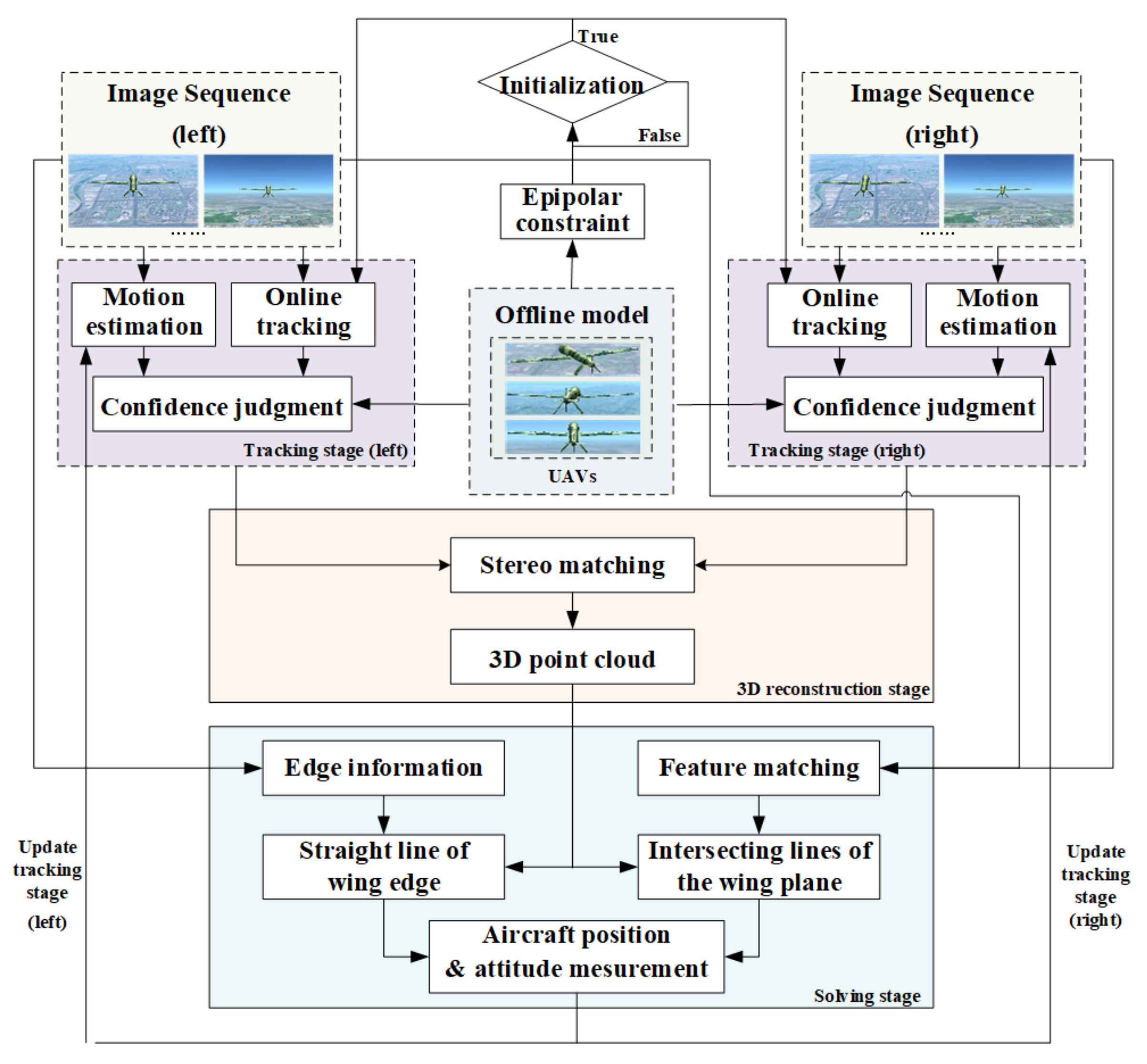
2.2. Proposed Architecture

The position and attitude measurement of UAVs is mainly used for formation flying and autonomous refueling in the air. During this process, the rear aircraft must sail at a speed slightly faster than that of the front aircraft. The two aircraft are constantly approaching, and the observation angle and relative distance between them may change remarkably over the course of flight. Thus, measuring the relative distance and attitude between the two aircraft is necessary to ensure safe navigation.
This paper focuses on the online measurement of the position and attitude of short-range UAVs. The measurement system is shown in Figure 2. Two cameras are placed on the rear machine, video streams acquired by cameras are used as input. Our method solves the pose of the front UAV by each pair of images.
The algorithm fuses 3D point cloud data with 2D information, such as image edges and feature points. Two cameras complete the acquisition of target images. Aircraft target positioning and tracking and 3D reconstruction are completed in the image. The set of points on the wing edge and plane are extracted according to the 3D point cloud and 2D images, and the straight-line equation of the wing edge space, the intersection line of the two wing planes, and the position of the front aircraft tail are subsequently calculated. Integrating the straight-line equation of the wing edge and the plane’s intersection line realizes the calculation of the three attitude angles. In the next section, the specific implementation of the proposed method will be described in detail.

3. Research Methodology

The algorithm proposed in this paper is divided into four parts, namely the initial stage, the tracking and positioning stage, the 3D reconstruction stage, and the pose calculation stage. The algorithm framework is shown in Figure 3. In the initialization phase, the candidate region can use the pre-trained model to perform initial frame processing on the image and then apply the epipolar geometric constraints in stereo vision to detect the consistency of the candidate image. In the tracking and positioning stage, the pre-training model is used to detect the initial position of the target. The 3D positioning result obtained by the detection result, the online tracking result, the target motion estimation, and the stereo vision constitute a confidence determination formula. The confidence of the target and final position are then located. In the 3D reconstruction stage, the tracking and positioning areas are matched in the binocular camera, and, finally, the 3D data of the target area are formed. In the pose solution stage, 3D data and 2D information are combined. In the disordered 3D data, the key points on the wings and fuselage are screened and marked separately to form a key point set. The key point set is used to solve the intersection of the wing edge line and wing plane, and the space line is used to calculate the attitude angle of the target aircraft in three directions. Motion estimation and tracker module in the tracking stage can use the target position information obtained in the solving stage to update.

3.1. Initialization Stage

Before tracking and positioning, the tracking target needs to be initially positioned. In the initialization phase, an offline trained classifier (offline model) is used to find possible candidates in the image sequence that is input. Candidates we find are not all the region we want to track. Therefore, the candidate regions need to be filtered [20].
{ x l i t } i = 0 M is the candidate found in the t t h frame of the left image sequence. and { x r j t } j = 0 N is the candidate region found in the t t h frame of the right image sequence. M and N indicate the number of candidate regions detected. Each candidate area is x t = a t , b t , w t , h t , where a , b , w , h denotes the column and row coordinates of the top left corner and the width and height of the candidate, respectively. p l i and p r j are the center points of x l i t and x r j t , respectively. w l i and w r j are the widths of x l i t and x r j t , respectively [21].
In a fixed binocular system, the target is a single-target detection. Therefore, in the corresponding frame, in the M candidate regions { x l i t } i = 0 M and N candidate regions { x r j t } j = 0 N corresponding to all the left and right images, only one pair of candidates should satisfied the following conditions: widths of candidates w l i and w r j should satisfied w l i w r j < 0.05 × m a x ( w l i , w r j ) . Based on the epipolar, the constraint shows that the relevant center points p l i and p r j of should be satisfied p r j T F p l i < ε (where F is the fundamental matrix and ε is a reliable threshold for judging). By applying binocular filtering, candidate in the image can be determined, and the other candidates that are incorrect are filtered out.

3.2. Tracking Stage

After the initialization is complete, the algorithm enters the tracking stage. For the corresponding frame in each image sequence, the target position is located through detection (that is, obtained by the offline classifier model), online tracking and motion estimation [22]. In this stage, the detection algorithm is the ADAboost algorithm [23] with haar feature. The tracking algorithm which used is KCF [24] with hog feature.
For the target in each image sequence, Kalman filtering [25] and the position and attitude of the target in the previous frame can be used to predict the current position of the target, and and the position of the motion estimation is represented as x k = ( a k , b k , w k , h k ) , where a k , b k , w k , h k denotes the column and row coordinates of the top left corner and the width and height of the motion estimation x k respectively. Furthermore, an ROI (region of interest) is generated around the estimated position for subsequent local detection, which is three times the size of the width w k and height h k .
The offline classifier is used to detect the target, and x d i i = 0 M is the candidate found in the current frame. Each candidate area is x d = a d , b d , w d , h d , where a d , b d , w d , h d denotes the column and row coordinates of the top left corner and the width and height of the candidate x d respectively. p d is the center point of x d . Furthermore, the spatial center position p c e n ( x c e n , y c e n , z c e n ) of the previous frame is calculated to be projected onto the image plane to obtain its coordinates p p c e n ( u p c e n , v p c e n ) .
The shape and position of the drogue do not mutate throughout the process. Therefore, the detection candidates which detected by detection algorithm close to the region given by the motion estimation have high confidence. The judgment of confidence of the detection candidate can be completed by the following:
c d = c d s · c d c · s
and c d s and c d c are defined as
c d s = min w d · h d , w k · h k max w d · h d , w k · h k
c d c = f p N a d , b d
where p N N a k b k , σ 2 0 0 σ 2 , of which σ = w k 2 + h k 2 . The function f is used to remap the value of p N within 2 σ of a k , b k to the interval [ 0 , 1 ] . s is also a normal distribution, which is given according to the distance from the center point p d to the projected point p p c e n , similar as c d c , here σ = u p c e n 2 + v p c e n 2 . If there are multiple candidates, the value with the highest confidence is selected as the detection result.
Similarly, the confidence judgment formula for online tracking is as follows:
c o = c o s · c o c · s
The parameter definition is similar to that in the confidence of the detection candidate.
For the positioning process of each frame, the target state can be defined as { x , c } , where x is the target position and c is the confidence of the position. Given motion estimation x k , detection x d and online tracking x o , the confidence evaluation function is as follows:
x , c = 0 , 1 if c d < θ 1 & c o < θ 2 x d , c d if c d θ 1 & c o θ 2 & c d c o if c d θ 1 & c o < θ 2 x o , c o if c d θ 1 & c o θ 2 & c d < c o if c d < θ 1 & c o θ 2
where θ 1 and θ 2 are the reliability thresholds of detection and tracking confidence, respectively. The confidence of detection and tracking is compared with a set reliability threshold to locate the current frame target. If the detection confidence is 0 for 20 frames, the confidence of the entire algorithm is considered to be 0, and the algorithm returns to the initialization stage.

3.3. 3D Reconstruction Stage
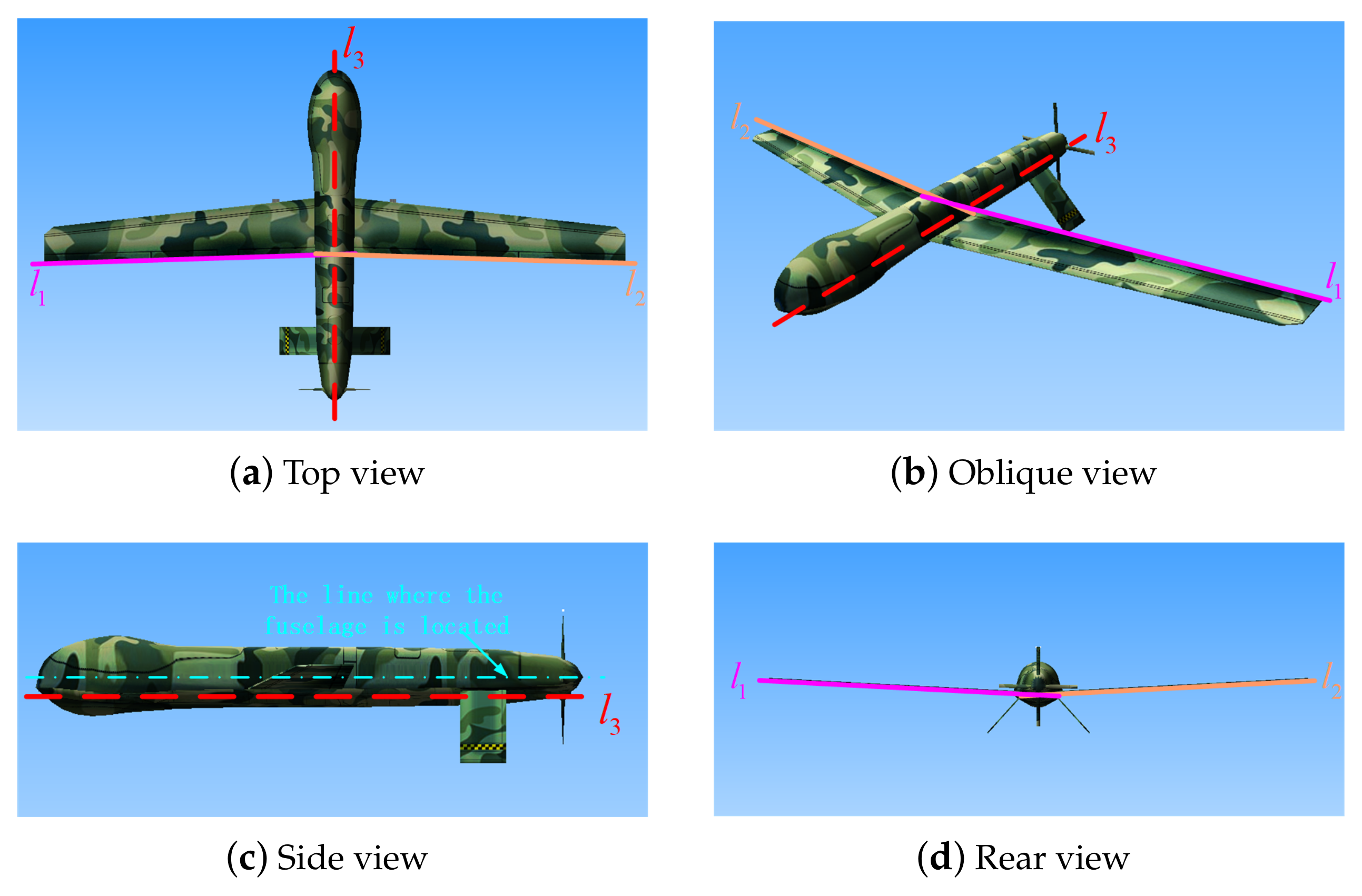
This study uses a semi-global matching algorithm to solve the disparity problem of input image pair [26]. The algorithm idea is to form a disparity map by selecting the disparity of each pixel. The global energetic function associated with the disparity map is set to minimize the energetic function to achieve the optimal goal of each pixel. The energetic function that depends on the disparity image D is as follows:
E D = p ( C p , D p + q N p P 1 T D p D q = 1 + q N p P 2 T D p D q > 1 )
where p and q represent pixels. D represents the disparity image. D P and D q represent the disparity between p and q, respectively. C p , D p is the matching cost of pixel p with respect to disparity D p , which can be solved by the sum of absolute differences. q is in the neighborhood N p of p, and its disparity changes slightly (that is, 1 pixel). The operator T   [ ] ) is the probability distribution of the corresponding intensity, which is 0 if its argument is false and 1, otherwise. P 1 and P 2 represent a penalty coefficient of 1 and a disparity difference greater than 1, respectively.
Solving using the energetic function in the Formula (6) is an NP-complete problem. It is approximated as multiple one-dimensional problems and solved by dynamic programming [27]. For example, considering the direction from left to right, each pixel is only related to its coordinate pixel. The formula is as follows:
L r p , d = C p , d + min L r p r , d , L r p r , d 1 + P 1 , L r p r , d + 1 + P 1 , min i L r p r , i + P 2 min k L r p r , k
where L r p , d represents the minimum cost of the current pixel when the disparity of the current pixel is d. Here, r can be understood as the neighboring pixels of the pixel p in this direction.
Costs in the eight directions are accumulated, and the smallest accumulated cost is selected as the final disparity of the pixel. The cumulative formula is expressed as follows:
S p , d = r L r p , d
A disparity map of the entire image can be obtained by performing the above operation for each pixel in image.

3.4. Solving Stage

Figure 4 shows an analysis of the airplane model. The space straight lines l 1 and l 2 where the rear edges of the left and right wings of the airplane are located are not collinear. Because the wing of the aircraft is symmetrical, according to the plane’s own coordinate system and the plane’s top view, the straight lines l 1 and l 2 are in the plane coordinate system O p x p y p z p in O p x p y p . The projected line on the plane has the same angle relative to the x p axis and is axisymmetric about y p . Therefore, the aircraft yaw angle can be solved according to the space straight lines l 1 and l 2 . According to the rear view and coordinate system of the aircraft, similar to the yaw angle solution, the roll angle of the aircraft can be calculated on the basis of the space straight lines l 1 and l 2 . The projections of the space straight lines l 1 and l 2 on the O p y p z p plane are challenging to distinguish and easily affected by noise; thus, the pitch angle is unstable. From our analysis of the side view of the aircraft, the intersection line of the left and right wing planes l 3 on the O p y p z p plane is parallel to the fuselage line. Therefore, the pitch angle of the aircraft can be solved by the angle between this intersection and the plane.
In summary, the process of solving the 3D attitude angle of the aircraft is transformed into the process of solving the space straight lines l 1 and l 2 where the rear edges of the left and right wings of the aircraft are located, and the intersection line l 3 of the two wing planes.
The proposed method uses the disparity map I d to obtain the target area of the aircraft and then count the points in this map according to the columns. The disparity map can be divided into three regions according to the number of corresponding points in the columns, namely, the left wing region I d l , the fuselage area I d c , and the right wing area I d r .
The proposed method extracts the edge space points of the left wing of the aircraft, that is, filter the edge point set in the left wing area. Next, the proposed method calculates the corresponding depth map I d e p t h l according to the disparity map I d l . Because the wing area is projected on the image plane according to the perspective projection, the order of the wing part in each column of the image is from far to near. The input image has a one-to-one correspondence with the disparity map; thus, the left wing edge point set { p e d g e l } can be filtered out according to the depth information of the corresponding points obtained by the disparity map calculation. In the process of screening the edge point set, the proposed method can judge whether the selected point is a noise point according to the depth information in the neighborhood and the ordinate position of the point in the image and filter out the relevant noise point.
The proposed method projects the extracted left wing edge point set { p e d g e l } back to the image plane, as shown in the Figure 5a. The “holes” generated by the stereo matching algorithm can be clearly seen and lead to extraction The resulting edge point set is discontinuous and mixed with some non-edge points on the wing; such features can cause great errors in solving the straight-line equation of the edge of the aircraft wing. Therefore, the proposed method combines the edge features of the image, correct each point in the left wing edge point set { p e d g e l } , and then correct the noise points back to the accurate edge to obtain an accurate set of wing edge points { p e d g e l } . The effect is shown in Figure 5b. Canny algorithm [28] is used in image edge detection.
According to the point set { p e d g e l } fit the space straight line L e d g e l on the edge of the left wing:
x x e d g e l A e d g e l = y y e d g e l B e d g e l = z z e d g e l C e d g e l
Similar to the above solution process, the corresponding depth map I d r is calculated for the right wing area I d e p t h r , and the right wing edge space point set { p e d g e r } is obtained. The fitting is the edge space line of the right wing L e d g e r :
x x e d g e r A e d g e r = y y e d g e r B e d g e r = z z e d g e r C e d g e r
According to the linear equations of L e d g e l and L e d g e r , the angles φ e d g e l and φ e d g e r between their projection lines in O p x p y p of the aircraft coordinate system (i.e., O x z plane of the camera coordinate system) and the axis of x can be solved. Given the symmetrical properties of the wings, the initial state angle can be defined as φ 0 , and the yaw angle of the aircraft is φ . The corresponding relationship is shown in Figure 6:
Because the angles between the two linear space vectors and the positive direction of the x axis are acute, the formula for calculating the yaw angle φ of the aircraft is as follows:
φ = φ e d g e r + φ e d g e l 2 if C e d g e l · C e d g e r 0 φ e d g e r φ e d g e l 2 if C e d g e l · C e d g e r < 0
The aircraft pitch angle θ is solved by the intersection of the two wing planes. Although the disparity map I d can be divided into the wing area and the fuselage area, errors may be encountered during the process of fitting the plane because a large number of noise points in the 3D point cloud are calculated in the stereo matching algorithm. Moreover, because the amount of point cloud data is large, the calculation efficiency of the method may be negatively affected. Therefore, this paper uses the spatial point set formed by the feature points in the wing area to fit the plane and calculate the intersection of the wing plane. Here, the proposed method use the disparity map I d and its area distinction to filter the matching feature points, constrain the matching of the feature points through the disparity (i.e., depth information) corresponding to the feature points, eliminate the incorrectly matched points on the same horizontal line, as shown in Figure 7. The feature used in the image is ORB feature [29].
The feature points extracted from the corresponding left image through the left wing area I d l in the disparity map are divided. The feature point p f e a l i l = ( u f e a l i l , v f e a l i l ) in the left wing area and the feature point in the right image that matches this feature point p f e a l i r = ( u f e a l i r , v f e a l i r ) are extracted, where u f e a l i and v f e a l i denotes the column and row coordinates of the feature point p f e a l i respectively. For comparison, the proposed method can filter out the feature point set on the left wing { p f e a l } . The filter formula is as follows:
f ( x ) = p f e a l i l { p f e a l i } if | u f e a l i r u f e a l i l | < δ & & p f e a l i l I d l p f e a l i l { p f e a l } else
The 3D coordinates of each point in the feature set { p f e a l } are calculated, and the plane equation of the left wing is fitted as follows:
A w i n g l x + B w i n g l y + C w i n g l = z
In the same way, the feature point set on the right wing { p f e a r } can be extracted through the above process, and the right wing plane equation can be fitted as shown below:
A w i n g r x + B w i n g r y + C w i n g r = z
The normal vectors M w i n g l and M w i n g r of the plane where the two wings are located are obtained, and the cross product are used to calculate the direction vector M l 3 of the plane intersection l 3 .
M l 3 = M w i n g l × M w i n g r
The angle between the projection of the direction vector M l 3 of the plane intersection line l 3 in O p y p z p plane of the aircraft coordinate system (i.e., O y z plane of the camera coordinate system) and the y axis of the aircraft coordinate system (i.e., the z axis of the camera coordinate system) is the pitch angle θ of the aircraft.
According to the conventional aircraft shape, the position of the aircraft can be spatially located through the tail of the aircraft. The point with the smallest depth information is found in the fuselage area I d c in the disparity map. The difference between the disparity of the point in the adjacent area is used to eliminate the noise points, and the position p t a i l x t a i l , y t a i l , z t a i l of the tail of the aircraft is obtained.
The proposed method is presented in Algorithm 1. After calculating the aircraft’s space pose, its position information will be adopted to update the confidence of the tracking stage.
Algorithm 1: Measuring Position and Orientation of Aircraft.
Input: Frame Sequence
Output: Location p t a i l , Pitch θ , Roll γ and Yaw φ
while not end of sequence do
Applsci 11 01373 i001

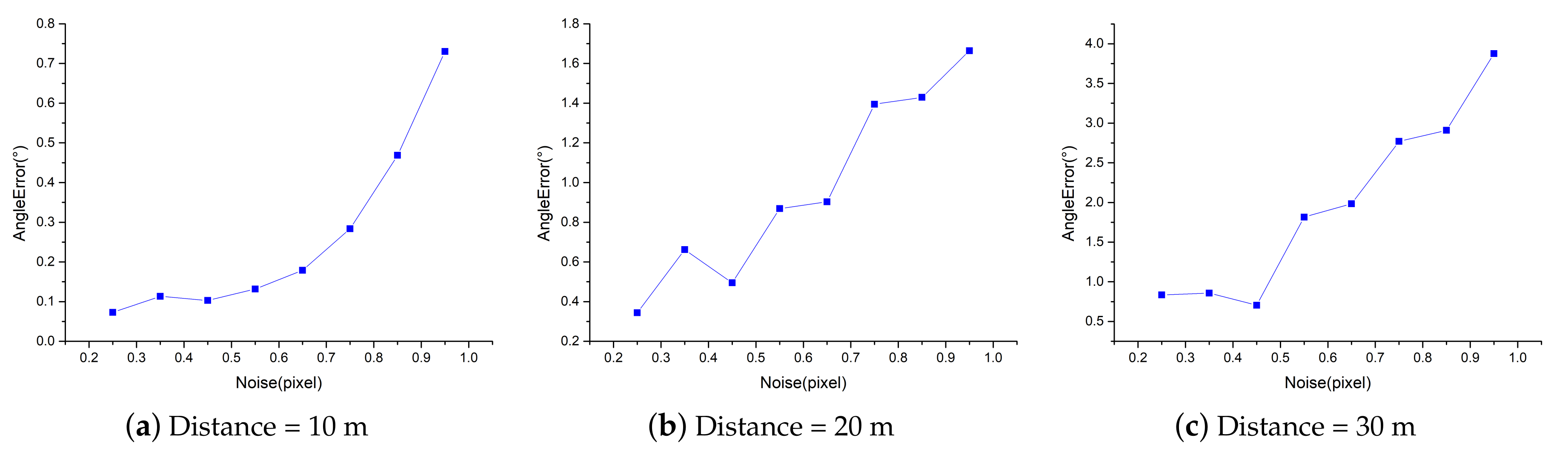
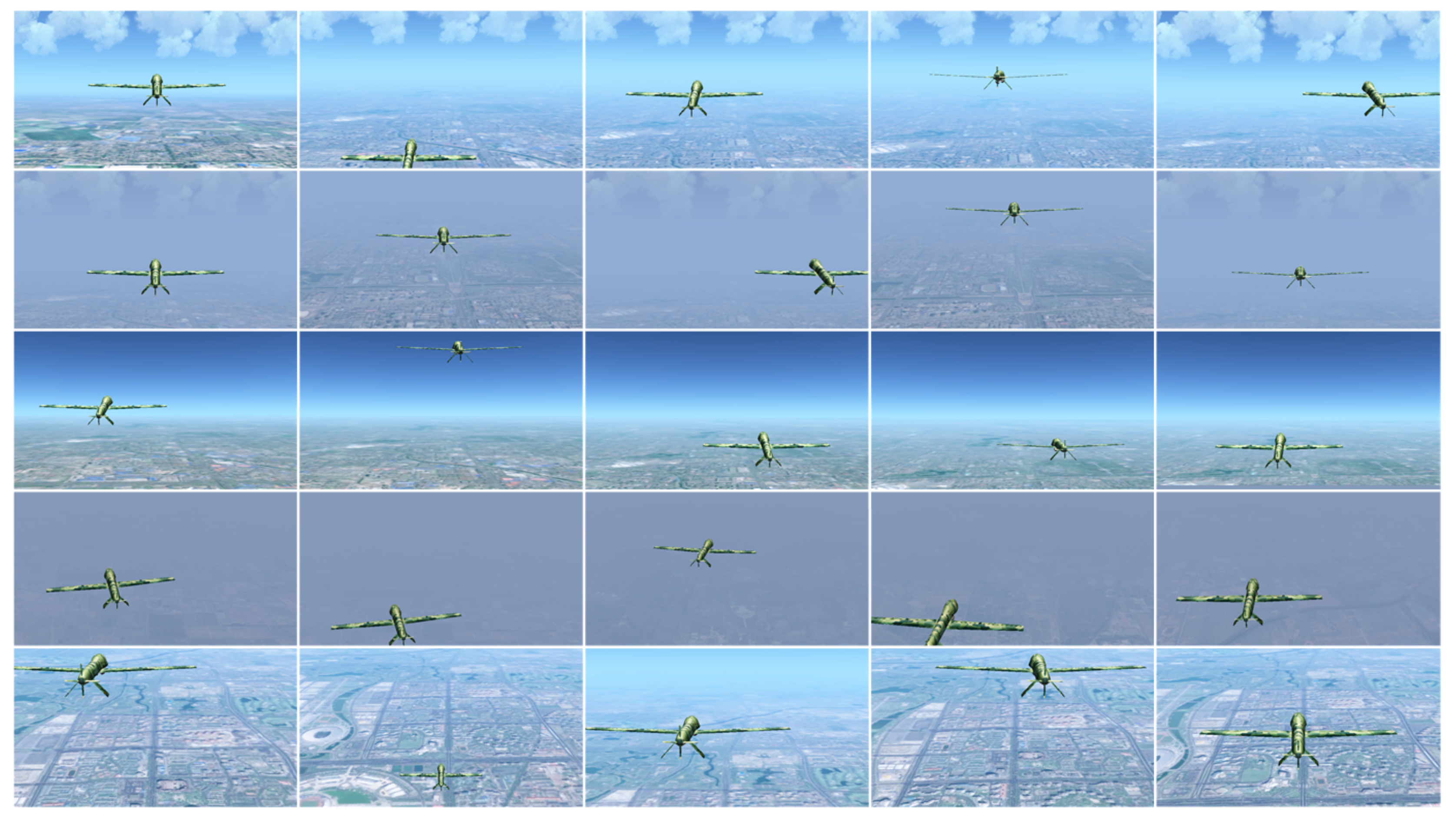
4. Simulation Experiment

Plane fitting in the pose measurement process may exert a great impact on the accuracy of the method. Therefore, a simulation experiment is carried out on the plane fitting method. A plane is constructed in the space, several points in the plane are projected onto the corresponding plane of the binocular camera, noises of 0.25, 0.5, and 1 pixel are added to the image plane points, and the method is verified. In different noise environments, within the range of 10 to 32 m, the error is between the solved plane and the constructed plane equation. Figure 8a shows the result of the method obtained under a 0.25-pixel noise. The angle error is approximately 1 within 32 m. Figure 8b shows the result of the method obtained under a 0.5-pixel noise. The results show that the error basically increases as the distance increases. The error reaches 2 . 38 . Figure 8c shows the result of the method obtained under a 1-pixel noise. The error reaches 2 . 44 at 25 m. At 32 m, the error is close to 4 , which exerts a greater impact on the measurement accuracy.
Corresponding to the experimental conditions, the pixel noise is used as a variable, and simulation experiments are performed at 10, 20, and 30 m, as shown in Figure 9. Figure 9c shows that at 30 m, after the error of more than 0.65 pixels, the angle error has exceeded 2 ; when the noise is close to 1 pixel, the angle error is close to 4 , which echoes the previous experiment.
In summary, the simulation experiment shows that the matching error must be reduced as much as possible to meet actual needs. This error should ideally be controlled to 0.5 pixels, that is, the angle error is controlled at about 2 , which can better meet the demand.

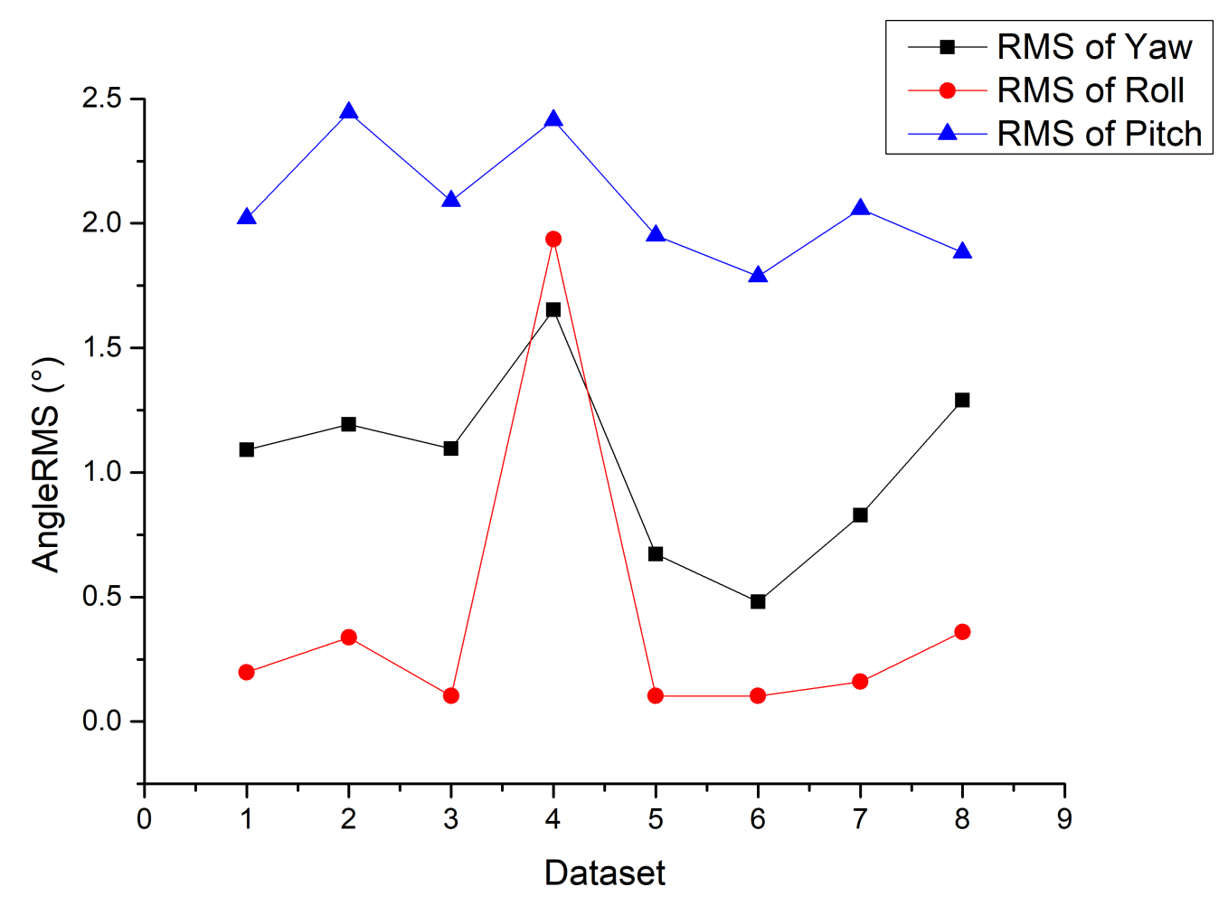
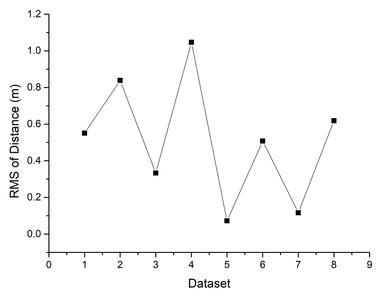
5. Physical Experiment

In this section, the complete experiment process and analysis are discussed. We then introduce the experimental environment, datasets, and experimental procedure.

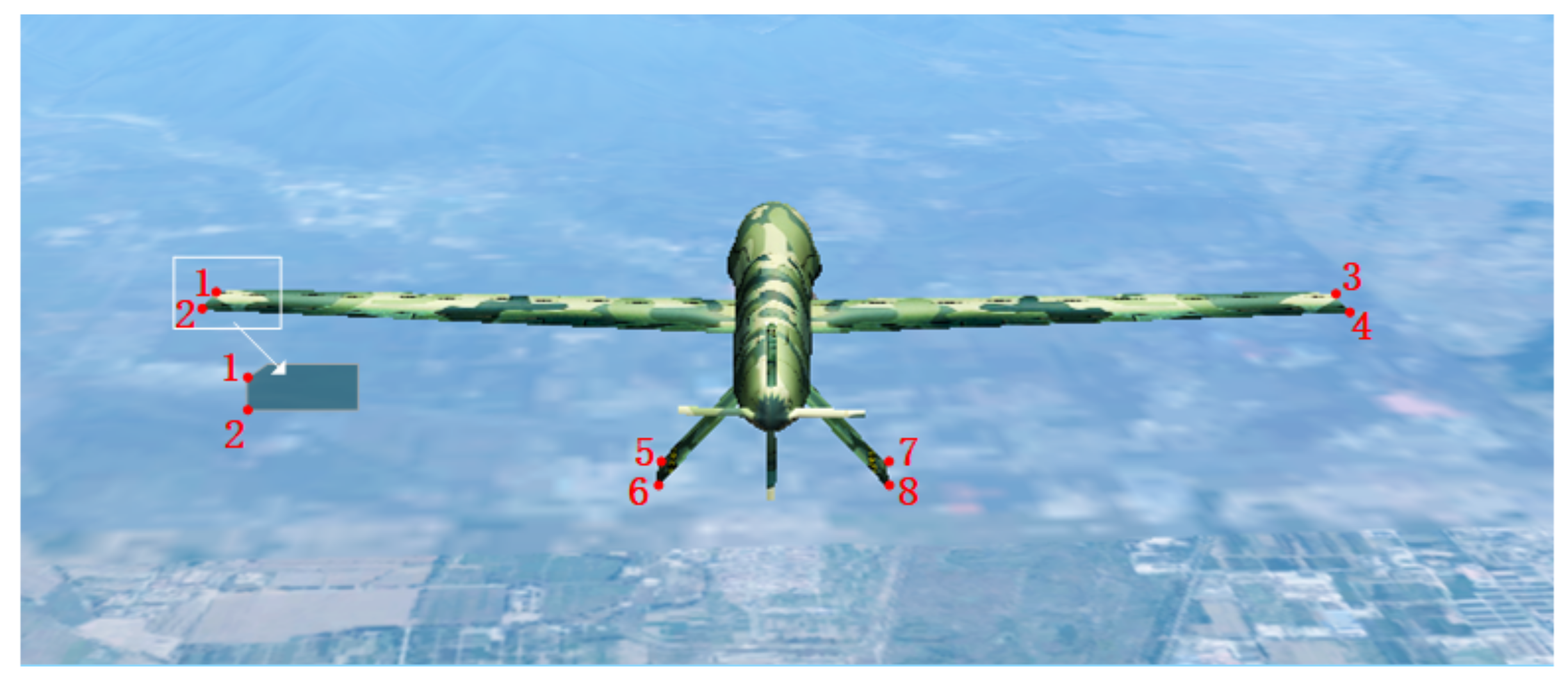
5.1. Implementation Details

The algorithm in this paper is verified on a digital simulation platform. The visual simulation software used for display can simulate the effect of UAV navigation in various geographical environments, altitudes, and weather environments. The image sequence outputted by the simulation software can simulate the images taken by the dual cameras and output the true values of the real position and attitude. These images can be used as datasets to verify and compare measurement methods for the position and attitude of the UAV. Because of the limited parameters in the simulation software, the roll angle of the aircraft attitude is set to a fixed value of 0.
The dataset used is shown in Figure 10:
The proposed method is written in vs2013+OpenCV 2.4.13 using C++ and ran on a computer with an Intel i7-6820HQ (2.7 GHz) CPU, 16 GB RAM, and an NVIDIA Quadro M2000M GPU. The resolution of the image sequence collected by the simulated binocular stereo vision system is 888 × 500 pixels. The internal parameters of the virtual camera are fixed, the focal length is a x = a y = 1080 pixels, the principal point coordinates are ( u 0 , v 0 ) = ( 444 , 250 ) pixels. The rotation matrix in the stereo vision system is the identity matrix, the translation vector is T = ( 0 , 0 , 1000 ) mm.
The proposed method in this study is formed by the combination of motion estimation, an offline model, and online tracking. The proposed method uses ADAboost [23] with the haar feature as the offline model and KCF [24] with the hog feature as the online tracking algorithm. Some parameters must be set in each stage of the proposed method. During classifier pre-training, the number of stages is set to 20 based on experience. The minimum detection rate of each class of strong classifier is set to 0.999. In the tracking component, the linear interpolation factor for adaptation is set to 0.012 and the Gaussian kernel bandwidth is set to 0.6. In the solving stage, the method of feature extraction is ORB feature [29]. Other parameters are set to default values.

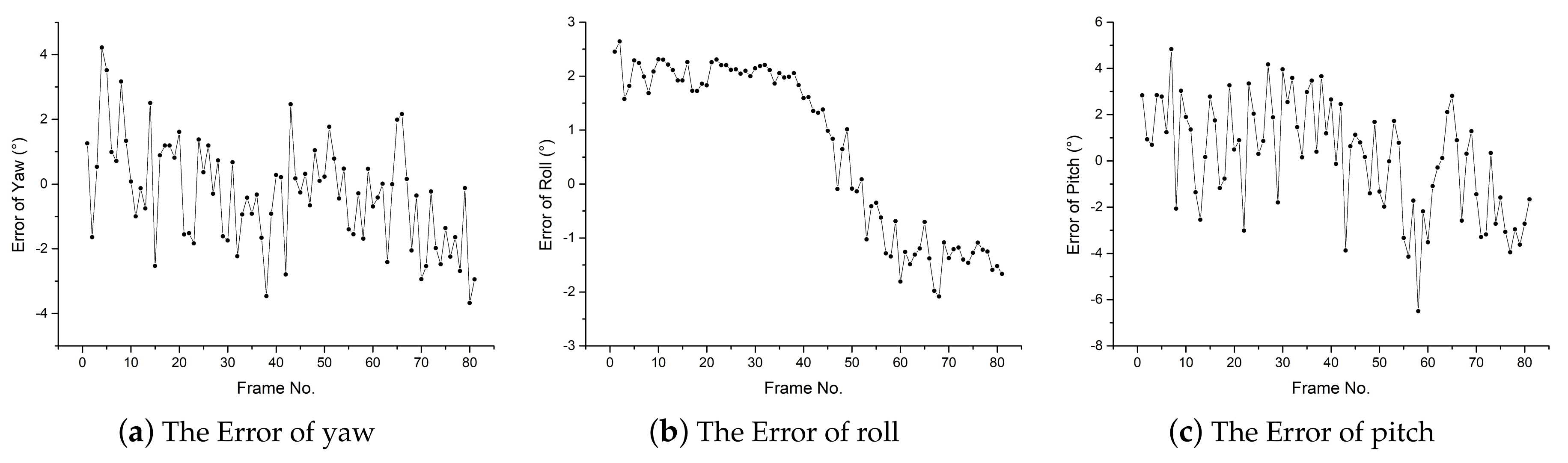
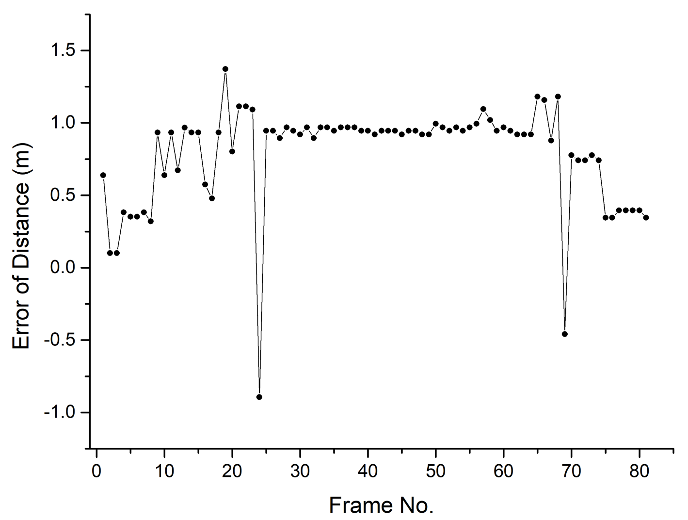
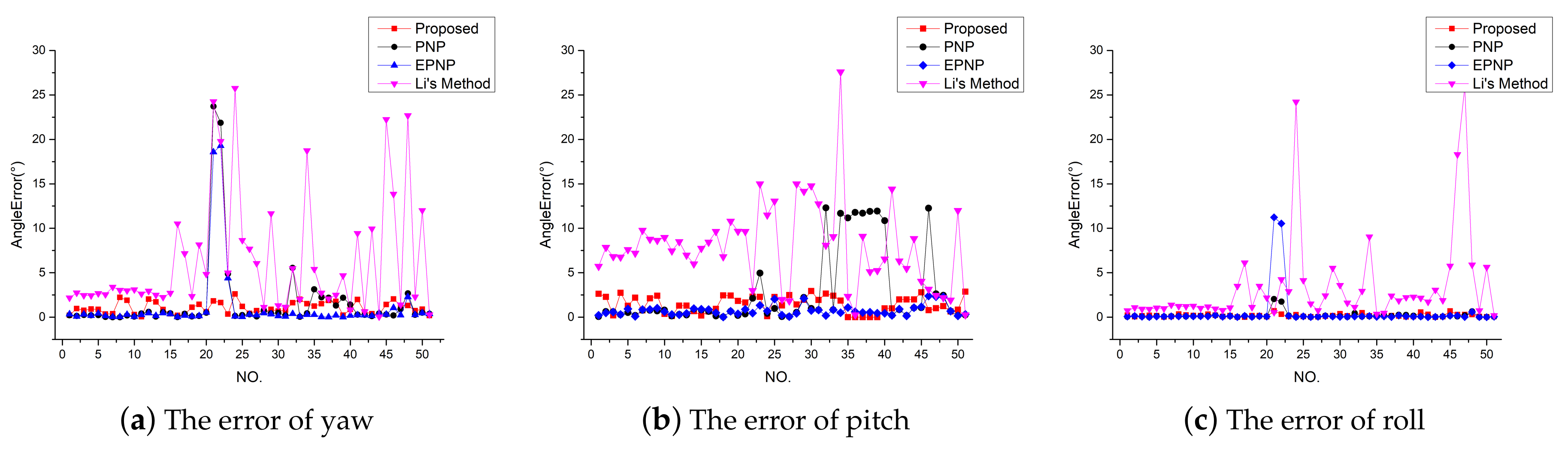
5.2. Measurement Accuracy Evaluation

This article considers different weather conditions, angles, and flying altitudes (i.e., different backgrounds) and collects eight datasets, including aircraft out of view and partial occlusion, among others. The measurement distance is approximately 14–33 m. The aircraft pose was measured on these eight datasets and compared with the real values recorded by the visual simulation software. The attitude angles and distance RMS values of the eight datasets are shown in Figure 11 and Figure 12, respectively.
Figure 13 shows the error values of the three attitude angles of some measurement data. In most datasets, the RMS of the roll angle is small and stable within 0.5 . However, in some of the datasets, the error of the roll angle is relatively large because of the influence of the background environment and other attitude angles. In this case, the RMS may reach 1.9 . The RMS of the yaw angle is stable at approximately 1.0 but may occasionally be as high as 1.7 . The error of the pitch angle is the largest among the errors of the three attitude angles. In most datasets, the RMS of the pitch angle is stable at approximately 2.0 ; in some datasets, the values obtained may rise to 2.5 . In summary, the RMS of most of attitude angles which calculated by the proposed method is within 2.0 between 14 and 33 m.
During the determination of the relative position of UAVs, distance, that is, the depth direction in the camera coordinate system, is the most important measurement. The proposed method calculates the distance between drones in each dataset. In all datasets, the RMS of the distance measurement result is 0.61 m. The data in Figure 12 show that most of the RMS values of the distance measurement results in all datasets are within 0.84 m. Only one dataset, where the true distance is approximately 25–30 m, has an RMS of 1.08 m. Figure 14 shows the RMS values of the results in this dataset. Our findings indicate that the proposed method can be used for collision avoidance measurements when the aircraft is sailing in the air.
The aircraft attitude angles calculated by the proposed method are shown in Table 2. The error contrast between the yaw angle measured by the proposed method and the true value is relatively small and remains within 1.5 . The error of the roll angle is clearly distinguished. When the actual yaw angle is small, the measurement error of the roll angle is small. When the yaw angle is large, the measurement error of the roll angle is large, but the RMS remains within 2 . The error of the pitch angle is well within a stable range, and most of the measurement errors are within approximately 2.00 . While some measurement values are occasionally greater than 2.5 , which could affect the measurement accuracy to a certain extent, it will not bring devastating results and the safety of aircraft navigation can still be ensured.
The method proposed in this paper is compared with conventional methods of calculating aircraft attitude, including PNP, EPNP [30], and Li’s method [31], to verify its validity and reliability. PNP is a traditional pose estimation algorithm, which estimates the pose of the target through multiple space points and their projection positions. Li’s method is based on parallel vision and uses the triangulation method for stereo matching and 3D reconstruction. Furthermore, the pose estimation algorithm of Li’s method is also widely used. So they were selected for comparison to validate our proposed method. In this experiment, eight key corners of the aircraft are artificially marked for the comparison algorithm to calculate the aircraft attitude. The speed of the measurement method in this paper is 12 fps. Because some data of other methods are extracted manually, the calculation speeds of the algorithms cannot be compared. The eight points extracted are shown in Figure 15.
The measured RMSEs of aircraft attitude angle and depth distance are shown in Table 3. The RMSE of the three attitude angles are 1.1 , 0.8 and 2.1 . The data show no large gap between the accuracy of the proposed method in this article and the comparison method, but the proposed method can be applied to the aircraft attitude when some key points, such as the wing and tail part, are blocked. In the case of the comparison method, the extracted 2D point data do not correspond to the 3D points, and large deviations in the measurement results are noted. These deviations present a safety hazard during the flight of the aircraft. Li’s method has the same accuracy as the proposed method in distance measurement, but it has a larger angle error in attitude measurement. In Li’s method, when calculating three-dimensional space points, a large error will be introduced because of the long distance of the object. The attitude is calculated through the corresponding three-dimensional points. So the result of attitude calculation is inaccurate.
Figure 16 shows some of the measured attitude angle data. The yaw and roll measured by the comparison algorithm produces serious errors in images 22 and 23. This error is caused by the UAV partially occluding the right wing in the image, which results in a corresponding point error. The pitch also shows obvious errors in images of 22–24, 34–40, and 46 because the wing plane is linearized in the image on account of the occlusion of the wing and the small pitch angle, thereby resulting in inaccurate lifting points. By comparison, the measured values of the proposed method are stable within a certain error range. This finding confirms the robustness and reliability of the proposed method.

6. Conclusions

Aimed at the flying formation and AAR of UAVs, this paper proposes a UAV pose measurement method based on rigid skeleton structure, which uses the spatial linear equation of rigid skeleton combined with the geometric model to solve the aircraft pose. This paper first proposes a key point extraction method that integrates 2D image data with 3D depth information to solve the problem of reduced feature point mismatch. This method improves the accuracy and stability of the pose measurement method. Compared with other methods, the proposed method in this paper can solve the problem of UAV attitude calculation without the need for auxiliary equipment, such as a theodolite, or remote transmission of data signals. Thus, the proposed method effectively improves the reliability and robustness of the pose measurement method and provides a safety guarantee for the aerial flight of UAVs. The proposed method can measure the position and attitude of UAVs without the need for knowledge of the aircraft model and size. The RMS error of the attitude angle is within 2.1 and the RMS error of distance measurement is within 0.61 m. The calculation frequency is 12 fps, which meets the collision avoidance measurement conditions of short-range UAVs in flight. The effectiveness and feasibility of the proposed method are verified in a simulation environment. The proposed method does not have a complex framework, which is easy to be implemented and used in actual project engineering.

Author Contributions

Conceptualization, J.Z. and Z.L.; methodology, J.Z.; software, J.Z.; validation, J.Z.; data analysis, J.Z.; writing–original draft preparation, J.Z.; writing–review, Z.L and G.Z.; supervision, Z.L; project administration, Z.L. and G.Z.; funding acquisition, G.Z. All authors have read and agreed to the published version of the manuscript.

Funding

This work was supported by Aviation Science Foundation Project (No:201946051001).

Institutional Review Board Statement

Not applicable.

Informed Consent Statement

Not applicable.

Data Availability Statement

Data available on request due to restrictions eg privacy or ethical.

Conflicts of Interest

The authors declare no conflict of interest.

Abbreviations

The following abbreviations are used in this manuscript:
UAVUnmanned Aerial Vehicle
AARAutomated Aerial Refueling

References

  1. Chiang, K.W.; Tsai, M.L.; Chu, C.H. The Development of an UAV Borne Direct Georeferenced Photogrammetric Platform for Ground Control Point Free Applications. Sensors 2012, 12, 9161–9180. [Google Scholar] [CrossRef] [PubMed] [Green Version]
  2. MartínezdeDios, J.R.; Merino, L.; Ollero, A.; Ribeiro, L.M.; Viegas, X. Multi-UAV Experiments: Application to Forest Fires. Springer Tracts Adv. Robot. 2007, 37, 207–228. [Google Scholar]
  3. Chao, Z.; Zhou, S.L.; Ming, L.; Zhang, W.G. UAV Formation Flight Based on Nonlinear Model Predictive Control. Math. Probl. Eng. 2012, 2012, 181–188. [Google Scholar] [CrossRef]
  4. De Marina, H.G.; Espinosa, F.; Santos, C. Adaptive UAV Attitude Estimation Employing Unscented Kalman Filter, FOAM and Low-Cost MEMS Sensors. Sensors 2012, 12, 9566–9585. [Google Scholar] [CrossRef] [Green Version]
  5. Gross, J.; Gu, Y.; Rhudy, M. Fixed-Wing UAV Attitude Estimation Using Single Antenna GPS Signal Strength Measurements. Aerospace 2016, 3, 14. [Google Scholar] [CrossRef] [Green Version]
  6. Michael, S.; Sergio, M. Coupled GPS/MEMS IMU Attitude Determination of Small UAVs with COTS. Electronics 2017, 6, 15–31. [Google Scholar]
  7. Koksal, N.; Jalalmaab, M.; Fidan, B. Adaptive Linear Quadratic Attitude Tracking Control of a Quadrotor UAV Based on IMU Sensor Data Fusion. Sensors 2018, 19, 46. [Google Scholar] [CrossRef] [Green Version]
  8. Christian, E.; Lasse, K.; Heiner, K. Real-Time Single-Frequency GPS/MEMS-IMU Attitude Determination of Lightweight UAVs. Sensors 2015, 15, 26212–26235. [Google Scholar]
  9. David, P.; Dementhon, D.; Duraiswami, R.; Samet, H. SoftPOSIT: Simultaneous Pose and Correspondence Determination. Int. J. Comput. Vis. 2004, 59, 259–284. [Google Scholar] [CrossRef] [Green Version]
  10. Fischler, M.A.; Bolles, R.C. Random Sample Consensus: A Paradigm for Model Fitting with Applications to Image Analysis and Automated Cartography. Commun. ACM 1981, 24, 381–395. [Google Scholar] [CrossRef]
  11. Hinterstoisser, S.; Lepetit, V.; Ilic, S.; Holzer, S.; Navab, N. Model Based Training, Detection and Pose Estimation of Texture-Less 3D Objects in Heavily Cluttered Scenes. In Asian Conference on Computer Vision; Springer: Berlin/Heidelberg, Germany, 2012; pp. 548–562. [Google Scholar]
  12. Liebelt, J.; Schmid, C.; Schertler, K. Viewpoint-Independent Object Class Detection using 3D Feature Maps. In Proceedings of the 2008 IEEE Computer Society Conference on Computer Vision and Pattern Recognition (CVPR 2008), Anchorage, AK, USA, 24–26 June 2008; pp. 978–986. [Google Scholar]
  13. Luo, J.; Teng, X.; Zhang, X.; Zhong, L. Structure extraction of straight wing aircraft using consistent line clustering. In Proceedings of the 2017 2nd International Conference on Image, Vision and Computing (ICIVC), Chengdu, China, 2–4 June 2017. [Google Scholar]
  14. Wang, B. Research on the Algorithm of Aircraft 3D Attitude Measurement. Ph.D. Thesis, Chinese Academy of Sciences University, Beijing, China, 2012. [Google Scholar]
  15. Li, G. Three-Dimensional Attitude Measurement of Complex Rigid Flying Target Based on Perspective Projection Matching. Ph.D. Thesis, Harbin Institute of Technology, Harbin, China, 2015. [Google Scholar]
  16. Haiwen, Y.; Changshi, X.; Supu, X.; Yuanqiao, W.; Chunhui, Z.; Qiliang, L. A New Combined Vision Technique for Micro Aerial Vehicle Pose Estimation. Robotics 2017, 6, 6. [Google Scholar]
  17. Zhang, L.; Zhu, F.; Hao, Y.; Pan, W. Optimization-based non-cooperative spacecraft pose estimation using stereo cameras during proximity operations. Appl. Opt. 2017, 56, 4522–4531. [Google Scholar] [CrossRef] [PubMed]
  18. Zhang, L.; Zhu, F.; Hao, Y.; Pan, W. Rectangular-structure-based pose estimation method for non-cooperative rendezvous. Appl. Opt. 2018, 57, 6164–6173. [Google Scholar] [CrossRef] [PubMed]
  19. Teng, X.; Yu, Q.; Luo, J.; Zhang, X.; Wang, G. Pose Estimation for Straight Wing Aircraft Based on Consistent Line Clustering and Planes Intersection. Sensors 2019, 19, 342. [Google Scholar] [CrossRef] [PubMed] [Green Version]
  20. Hu, M.; Liu, Z.; Zhang, J.; Zhang, G. Robust object tracking via multi-cue fusion. Signal Process. 2017, 139, 86–95. [Google Scholar] [CrossRef]
  21. Zhang, J.; Liu, Z. Tracking and Position of Drogue for Autonomous Aerial Refueling. In Proceedings of the 2018 IEEE 3rd Optoelectronics Global Conference (OGC), Shenzhen, China, 4–7 September 2018. [Google Scholar]
  22. Zhang, J.; Liu, Z.; Gao, Y.; Zhang, G. Robust Method for Measuring the Position and Orientation of Drogue Based on Stereo Vision. IEEE Trans. Ind. Electron. 2020. Early Access Article. [Google Scholar] [CrossRef]
  23. Yoav, F.; Robert, E.S. A Decision-Theoretic Generalization of On-Line Learning and an Application to Boosting. J. Comput. Syst. Sci. 1997, 55, 119–139. [Google Scholar]
  24. Henriques, J.F.; Caseiro, R.; Martins, P.; Batista, J. High-Speed Tracking with Kernelized Correlation Filters. IEEE Trans. Pattern Anal. Mach. Intell. 2014, 37, 583–596. [Google Scholar] [CrossRef] [Green Version]
  25. Kalman, R.E. A New Approach To Linear Filtering and Prediction Problems. J. Basic Eng. 1960, 82D, 35–45. [Google Scholar] [CrossRef] [Green Version]
  26. Hirschmuller, H. Stereo Processing by Semiglobal Matching and Mutual Information. IEEE Trans. Pattern Anal. Mach. Intell. 2008, 30, 328–341. [Google Scholar] [CrossRef]
  27. Bellman, R.E.; Dreyfus, S.E. Dynamic Programming; Dover Publications, Incorporated: New York, NY, USA, 2003; pp. 348–358. [Google Scholar]
  28. Canny, J. A Computational Approach to Edge Detection. IEEE Trans. Pattern Anal. Mach. Intell. 1986, PAMI-8, 679–698. [Google Scholar] [CrossRef]
  29. Rublee, E.; Rabaud, V.; Konolige, K.; Bradski, G. ORB: An efficient alternative to SIFT or SURF. In Proceedings of the International Conference on Computer Vision, Barcelona, Spain, 6–13 November 2012. [Google Scholar]
  30. Lepetit, V.; Moreno-Noguer, F.; Fua, P. EPnP: An Accurate O(n) Solution to the PnP Problem. Int. J. Comput. Vis. 2009, 81, 155–166. [Google Scholar] [CrossRef] [Green Version]
  31. Li, R.; Zhou, Y.; Chen, F.; Chen, Y. Parallel vision-based pose estimation for non-cooperative spacecraft. Adv. Mech. Eng. 2015, 7, 1687814015594312. [Google Scholar] [CrossRef] [Green Version]
Figure 1. Definition of aircraft attitude angle.
Applsci 11 01373 g001
Figure 2. Measuring system.
Applsci 11 01373 g002
Figure 3. Framework of the proposed method.
Applsci 11 01373 g003
Figure 4. Schematic diagram of aircraft attitude measurement.
Applsci 11 01373 g004
Figure 5. Edge point set projection.
Applsci 11 01373 g005
Figure 6. Relationship between yaw and straight line projection.
Applsci 11 01373 g006
Figure 7. Feature points after filtering.
Applsci 11 01373 g007
Figure 8. The error of the angle
Applsci 11 01373 g008
Figure 9. The error of the angle.
Applsci 11 01373 g009
Figure 10. Aircraft attitude measurement datasets.
Applsci 11 01373 g010
Figure 11. The attitude RMS of datasets.
Applsci 11 01373 g011
Figure 12. The distance RMS of datasets.
Applsci 11 01373 g012
Figure 13. Error of attitude angle.
Applsci 11 01373 g013
Figure 14. Error of distance.
Applsci 11 01373 g014
Figure 15. Aircraft attitude measurement keypoints.
Applsci 11 01373 g015
Figure 16. Attitude angle measured by comparison algorithm.
Applsci 11 01373 g016
Table 1. Classification of pose measurement methods.
contact measurementGNSSIn ref. [5,6], GNSS is used to solve the aircraft pose, but the data update frequency of GNSS is slow, and the signal transmission is easily affected.
(attitude internal measurement)IMUIn ref. [7,8], IMU is used to calculate aircraft pose, but the positioning error of IMU increases with time, and the long-term accuracy is poor.
Ref. [9] proposed SoftPOSIT, which can solve pose parameters iteratively.
Ref. [10] proposed the N-point perspective problem, which is a PNP problem.
MonocularRef. [11] proposed a method to generate a template to estimate the target pose.
non-contact measurement Ref. [12] performed pose measurement based on contour matching method.
Ref. [13] recognized the lines of aircraft to realize the structure extraction.
Ref. [14] proposed a method to solve aircraft pose by using the line feature.
(attitude external measurement)Ref. [15] proposed a method to compare simulated images with real model.
Binocular or multiocularRef. [16] proposed a combined vision technology based on a multi-camera.
Refs. [17,18] proposed optimization-based methods to estimate aircraft pose.
Ref. [19] extracted and clustered image line features to solve aircraft pose.
Proposed Method proposes pose measurement based on rigid skeleton.
Table 2. Measurement result of attitude angle.
NO.Measurement Result( )True Value( )Error( )
YawPitchRollYawPitchRollYawPitchRoll
1−0.917.70.20.015.00.0−0.92.70.2
20.7−9.70.10.0−9.00.00.7−0.70.1
3−12.225.1−2.3−13.223.70.01.01.4−2.3
4−16.323.61.5−14.820.80.0−1.52.81.5
5−3.525.51.8−4.124.20.0−0.61.31.8
61.321.6−0.40.020.00.01.31.6−0.4
7−9.824.4−2.1−8.223.50.0−1.70.8−2.1
82.021.81.32.323.60.00.3−1.81.3
95.720.7−1.95.523.30.00.2−2.6−1.9
105.521.02.17.723.10.0−2.2−2.12.1
11−0.613.5−0.20.011.00.0−0.62.5−0.2
121.67.90.30.06.00.01.61.90.3
Table 3. RMS of attitude angle and depth distance in the comparison method.
MethodRMSE of Yaw ( )RMSE of Pitch ( )RMSE of Roll ( )RMSE of Distance (m)
Proposed1.12.10.80.61
EPNP2.00.81.81.33
PNP2.42.70.30.31
Li’s Method4.63.24.70.57
Publisher’s Note: MDPI stays neutral with regard to jurisdictional claims in published maps and institutional affiliations.

