Article

A Multiobjective Decision-Making Model for Risk-Based Maintenance Scheduling of Railway Earthworks

1
Infraplan Konzalting, 10000 Zagreb, Croatia
2
Department of Construction Management and Engineering, Faculty of Engineering Technology, University of Twente, 7522 NB Enschede, The Netherlands
3
Department of Industrial Engineering & Innovation Sciences, Information Systems, University of Eindhoven, 5612 AZ Eindhoven, The Netherlands
4
Centre for Infrastructure, Geotechnical and Water Engineering Research (IGWE), Department of Architecture and Civil Engineering, University of Bath, Bath BA2 7AY, UK
5
Faculty of Civil Engineering and Geosciences, Delft University of Technology, 2628 CD Delft, The Netherlands
*
Author to whom correspondence should be addressed.
Appl. Sci. 2021, 11(3), 965; https://doi.org/10.3390/app11030965
Submission received: 17 December 2020 / Revised: 14 January 2021 / Accepted: 17 January 2021 / Published: 21 January 2021

Abstract

:
Aged earthworks constitute a major proportion of European rail infrastructures, the replacement and remediation of which poses a serious problem. Considering the scale of the networks involved, it is infeasible both in terms of track downtime and money to replace all of these assets. It is, therefore, imperative to develop a rational means of managing slope infrastructure to determine the best use of available resources and plan maintenance in order of criticality. To do so, it is necessary to not just consider the structural performance of the asset but also to consider the safety and security of its users, the socioeconomic impact of remediation/failure and the relative importance of the asset to the network. This paper addresses this by looking at maintenance planning on a network level using multi-attribute utility theory (MAUT). MAUT is a methodology that allows one to balance the priorities of different objectives in a harmonious fashion allowing for a holistic means of ranking assets and, subsequently, a rational means of investing in maintenance. In this situation, three different attributes are considered when examining the utility of different maintenance options, namely availability (the user cost), economy (the financial implications) and structural reliability (the structural performance and subsequent safety of the structure). The main impact of this paper is to showcase that network maintenance planning can be carried out proactively in a manner that is balanced against the needs of the organization.

1. Introduction

Traditionally rail infrastructure asset maintenance has been performed retroactively to correct, through replacement or remediation, failed elements. Naturally, this carries substantial safety implications for end-users and financial liability for infrastructure owners [1]. To limit their exposure, infrastructure owners have been trying to move towards more proactive asset maintenance approaches [2,3,4]. Such an approach would allow them to invest money in a prudent, sensible fashion, which maximizes utility and subsequently gives the best return on their investment [5]. Resulting in safer infrastructure which offers greater value to consumers and owners alike with less investment of resources [6]. Unfortunately, it is seldom clear how to most effectively allocate resources to achieve these goals.
Railway networks are a significant global asset, with an estimated 200,063 km of track [7] in the EU alone, 95% of which was built before 1905. Individual structures along these railways, including bridges, tunnels and earthworks, were constructed prior to the advent of modern design and construction standards. Given their age, many have far exceeded typical design lifetimes, and their resilience to the impacts of increased traffic loading and extreme weather events is lower than comparable assets on modern networks like highways. Bridges and tunnels are discrete, high-value, visible assets, where the majority of safety problems are relatively easy to detect, and thus, budgets can be assigned with some certainty. As a result, these assets have undergone regular remediation and replacement since their initial construction, while most earthworks remain in their original condition [3]. This is problematic on several levels as the present-day structures are now carrying loads far above what was originally intended as part of everyday operation, while their long lifespans have left them at increased risk of deterioration from aging effects and extreme climate scenarios [8]. Aged embankments, in particular, due to their steep construction, are more susceptible to rainfall-induced shallow failures than their modern-day equivalents [9,10]. This is because embankments constructed at slope angles in excess of their internal angle of friction rely on cohesion and matric suction for stability, the latter of which is inversely proportional to soil moisture [11,12]. As a result, shallow shear failures often occur after heavy or prolonged rainfall [13]. Loveridge et al. [14] found a strong correlation between earthwork failure and monthly rainfall in excess of the long-term average.
Earthworks are often covered by vegetation, and their behavior varies temporally, being strongly influenced by both rainfall and drying events [15,16,17,18]. The situation is complicated further by the scope of the networks involved and the presence of steep earthworks made of unknown material [19,20,21]. As a result, it is difficult for infrastructure managers to make effective maintenance decisions that utilize allocated resources in an optimum fashion.
Although risk assessment for the management of earthwork slopes is now widely adopted, major failures are increasing [3]. This is partly due to issues such as aging, climate change and increased demand. However, an additional contributing factor is that current risk assessment approaches are overly reliant on the results of visual inspection for hazard assessment. When stability analyses are performed to compare the capacity (strength) to the demand (load), they tend to be deterministic with conservative estimates of input parameters. In reality, both the capacity and demand vary temporally in response to weather events and therefore, the choice of input parameters is neither straight-forward nor fixed, and a move towards probabilistic assessment where uncertainty is quantified to deliver a specific level of safety is preferred. The increased availability of data such as LiDAR for geometry, embedded sensor and satellite data combined with improved weather forecasts provides an opportunity for infrastructure managers to address this problem of quantifying safety and make better-informed maintenance investment decisions [22].
Having established the safety level, asset maintenance planning is a process of deciding the scope, timing, costs, and benefits of future maintenance activities on a specific asset. Due to long lifespans and constraints on budgets, optimization of maintenance investments considering technical and economic objectives is essential for railway owners to fulfill societal expectations. Implicit in any decision-making process is the need to construct, either directly or indirectly, the preference order so that alternatives can be ranked, and the best alternative can be selected [23]. For some decision-making problems, this may easily be accomplished. For example, in the case of a decision based on a cost-minimization rule (where the lowest-cost alternative is chosen), the preference order is adequately represented by the natural order of real numbers (representing costs). Multicriteria decision-making (MCDM) methods provide a systematic approach to evaluate multiple conflicting criteria in decision-making. Conflicting criteria are typical in evaluating options; for example, the cost is usually one of the main criteria, and some measure of quality (performance level) is typically another criterion, usually in conflict with a cost. MCDM is used to identify and quantify decision-maker and stakeholder considerations about various (mostly) non-monetary factors in order to compare alternative courses of action [24]. Alternatively, the multiple performance criteria can be combined into a so-called utility function, in which all the criteria are brought into a single scale.
This paper demonstrates the applicability of MAUT for proactively determining the optimum maintenance schedule of earthwork assets on a network scale. The approach is demonstrated using the Irish Rail network. Multiple performance objectives or goals are considered looking at a range of attributes, failure scenarios and maintenance options. The result is a ranking of a network’s earthwork maintenance schedule, in order of maximum return on investment, where the return is based on the tradeoff of multiple performance goals as selected by the infrastructure manager. An example would be to increase the structural safety and availability of a network while minimizing the cost of interventions [25,26,27,28]. It allows for the consideration of environmental impacts and user costs and can easily be augmented further by additional performance goals as they become relevant. It explicitly allows the user to integrate choice and risk preferences.

2. Stability Assessment of Earthworks

In this section, we present an overview of the safety challenges faced by owners of aging earthworks and set-out a rational methodology to describe earthwork safety using reliability theory.

2.1. Slope Stability

The earthworks assets considered in this paper include cuttings; where the line is excavated below the existing ground level in either soil or rock (Figure 1a); and embankments where the line is carried above existing ground on man-made fill, usually soil (Figure 1b). Common problems causing instability of slopes are shallow translational landslides caused by high rainfall (Figure 1a,b), rock falls caused by freeze–thaw effects (Figure 1c), and deep-seated rotational failures caused by the construction of embankments over weak sub-soils (Figure 1d). The safety of earthworks is typically determined in a slope stability analysis.
Shallow translational landslides are usually triggered by near-surface changes in moisture content. In dry periods negative pore water pressure (suctions) develop in the near-surface soils, which contribute significantly to their overall stability. This suction transient and reduce during periods of rainfall or snowmelt. Assuming an infinite slope failure model, the factor of safety (FOS = capacity/demand) can be calculated as follows:
F O S = C + γ   h   cos 2   α   tan ϕ γ   h   cos α sin α
where γ is the unit weight of soil, h the wetting front depth (depth of infiltrated water), the friction angle of the soil ϕ and α, the slope angle, See Gavin and Xue [29]. In this simplified approach, the effective cohesion and matric suction are combined into the total cohesion, C.
The primary mechanism for deep rotational slip failures on railway networks is the presence of soft ground underlying an embankment. As a result, these failures tend to be geographically well-defined (e.g., in peatlands and delta regions) and are not significantly affected by climate hazards. As the depth of this failure mechanism is typically much larger than rainfall-induced failures, the volume of soil involved is much larger. The factor of safety is typically determined assuming a circular failure surface in which the failure surface is divided into a number of vertical slices, and moment equilibrium is considered [30]. The key inputs for the analysis are the slope geometry and shear strength parameters of the soil. The factor of safety of a slope subject to a rotational failure is as follows:
F O S = i = 1 n [ c i Δ x i + ( W i u i Δ x i ) tan ϕ i ] sec α i 1 + tan ϕ i tan α i / F O S   i = 1 n W i sin α i
where: Wi is the weight (kN) of the ith slice, αi is the inclination angle of the base of the ith slice, Δxi (m) is the ith slice width, ci (kPa) is the cohesion of the soil on the base of the ith slice, ui (kPa) is the pore water pressure at the base of the ith slice, and ϕi is the friction angle of the soil at the base of the ith slice, See Figure 2.
The stability of a rock slope depends on a number of internal (slope angle, geology, fracturing, etc.) and external parameters (weathering, tectonic events, human anthropogenic factors, etc.). The impact of freeze–thaw cycles on rockfalls is well documented, as water infiltrates into existing fractures, freezes and causes expansion of the fracture that may eventually lead to a rock wedge being dislodged from the mass. In this paper, a 2D rock wedge failure mode is considered, where the geometry of the critical failure surface is dependent on the slope geometry [31].

2.2. Reliability of Slopes

Because soils are naturally occurring materials, their properties vary spatially and temporally. Therefore, while simple limit equilibrium analyses such as those described in Section 3.1 can be performed to determine the factor of safety against slope failure, many of the input parameters needed for these analyses are highly variable. As a result, the FOS value obtained is critically dependent on assumptions made by the designer. For the case of shallow translational landslides, the specific uncertainties associated with this failure mode include; the variation of total cohesion when suctions reduce as a result of changes in water content during infiltration and difficulties in assessing the rate at which wetting front development occurs. The wetting front or failure surface depth is a function of many variables. These include the initial suction profile (which depends on the grain size properties and antecedent weather), the geometry of the slope and permeability of the soil, rainfall intensity and duration, among other factors. For the rotational failure mechanism, the key uncertainties are the shear strength parameters and the presence of local soft spots or buried features, stresses on the failure plane and location of the slip surface. For rock wedge failures, the key uncertainty relates to the fracture spacing and the impact of freeze–thaw cycles.
Probabilistic analysis offers a rational way for engineers to include uncertainty in their designs [32]. Instead of assuming deterministic (unique) values for variables, the full distribution of likely values is considered. The limit-state (performance) function, which compares the capacity (C) and demand (D), See Figure 3 is given by Equation (3).
g ( X ) = ( C D ) {   > 0 ,   s a f e   s t a t e = 0 ,   l i m i t   s t a t e   < 0 ,   f a i l u r e   s t a t e
The probability of failure is the area of the curve where demand exceeds capacity and the reliability index β is defined as the distance by which the mean or expected value of the performance function exceeds zero in units of its standard deviation, σ (Equation (4). As entire distributions are being used as inputs, reliability can either be determined through brute force computation using Monte Carlo or else approximated using mathematical optimization approaches such as First Order Reliability Methods [33], Second Order Reliability Methods [34], Genetic Algorithm [29], Particle Swarm Optimisation [35,36], etc. This paper utilizes a genetic algorithm approach, as recommended by Xue and Gavin [29], to determine the reliability index.
β = μ ( G ( X ) ) σ ( G ( X ) )

3. Multiobjective Decision-Making Model for Maintenance Planning

3.1. Model Description

MAUT is a multicriteria decision-making method [37], based on expected utility theory where the concept of a lottery is used to change the weightings of different attributes to determine the indifference point between different outcomes. The indifference point is the point where the expected values from different outcomes are the same. MAUT allows the decision-maker to strongly influence the preference order through the construction of utility functions, which further allows for the direct consideration of uncertainty. In the maintenance planning process, the uncertainty mainly originates from a lack of data and/or a lack of clear preferences from the stakeholders. These functions are real-valued functions that must be determined for each attribute, where the attributes chosen should represent the characteristics that the decision-maker in question deems important. After defining utility functions for each attribute, objectives and constraints need to be established. If the decision-maker has a personal preference regarding maximizing or minimizing the influence of a given attribute, relative weights can be ascribed. The individual utility functions are then combined into one utility function using the established relative weightings and any constraints set by the decision-maker. This single criterion is optimized to determine the best course of action. MAUT’s primary use is to choose the strategy in situations where a strategy must be implemented, but there is no clear indication of which path is of greatest value [26].
MAUT is a well-structured procedure designed to elicit utility functions from multiple attributes, implement relative weighting, and establish an objective ranking. There are several methods available to model an attributes utility, such as linear, log, exponential, logarithmic and quadratic [38]. In this paper, the exponential utility function [39] is utilized to capture the uncertainty in stakeholder preference and the risk tolerance of the decision-maker for slope maintenance planning, considering object reliability, economy and availability as performance criteria.
The step-by-step application procedure to implement MAUT on multiple objective maintenance planning problems is shown in Figure 4 and discussed in detail below, see Equations (5)–(8):
  • Assuming that the objectives of the maintenance planning and related attributes have been established, the first step is to compute a single utility function (SUF) for each attribute by applying the exponential utility functions [40,41] as follows:
U i ( x i ) = A B e ( x i R T )
where:
A = e ( M i n ( x i ) R T ) [ e ( M i n ( x i ) R T ) e ( M a x ( x i ) R T ) ]
B = 1 [ e ( M i n ( x i ) R T ) e ( M a x ( x i ) R T ) ]
R T i = C E i l n ( 0.5 U i ( M a x ( x i ) ) 0.5 U i ( M i n ( x i ) ) + A B )
where:
U i ( x i ) = Single utility value for attribute i of a maintenance alternative x
A, B = Scaling constants;
e = The exponential constant, i.e., 2.718;
M i n ( x i ) = The exponential constant, i.e., 2.718;
M i n ( x i ) = Minimum value of attribute i across all alternatives;
M a x ( x i ) = Minimum value of attribute i across all alternatives;
RT = Risk tolerance.
When computing SUF, the scaling constants and RT are cyclically dependent. Equation (9) can be used with the goal seeker function of MS Excel [42] to solve this.
e C E R T = 0.5   e M a x ( x i ) R T + 0.5   e M i n ( x i ) R T
To obtain the exponential SUF, the decision-makers are presented with a lottery question of a maximum value (i.e., M a x ( x i ) ) and a minimum value (i.e., M i n ( x i ) ) of an attribute. The decision-maker must choose an indifference point between the best and the worst possible values, which is referred to as the certainty equivalent (CE). The average value between the best possible value or the worst possible value is referred to as the expected value (EV). The indifference point chosen by the decision-maker represents his/her attitude towards risk and risk tolerance. An indifference value where CE is equivalent to EV represents risk-neutral behavior. If the value of CE is lower than EV, the decision-maker has a risk-avoiding attitude, whereas the CE value greater than EV shows a risk-taking attitude. Consequently, a risk-avoiding attitude has a positive risk tolerance, while a risk-taking attitude has a negative risk tolerance value [43] (Caballero and Krishnamurthy, 2008). With the consideration of decision-makers’ uncertainty in eliciting indifference points, CE, under risk consideration, the final computed utilities of an attribute must lie between U ( M a x ( x i ) ) = 0, U ( M i n ( x i ) ) = 1.
2.
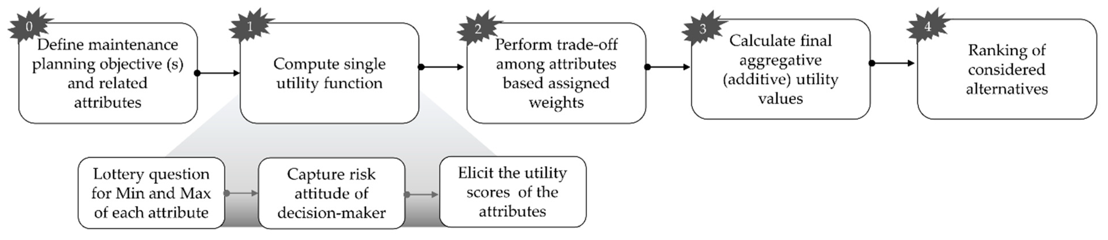
The next step is to perform tradeoffs among the attributes in order to find a solution that either maximizes or minimizes the stated performance goals or objectives. These tradeoffs characterize the relative importance of attributes for their defined objectives/performance goals. A direct rating method is applied to determine the weighting factors of the attributes, which is represented in Equation (10).
k ( x i ) = w ( x i ) i = 1 n w ( x i )
where:
k ( x i ) = Weighting factor of each attribute i across all alternatives;
w ( x i ) = weighting assigned by an expert for attribute i for maintenance activity x;
w ( x i ) = weighting assigned by an expert for attribute i for maintenance activity x.
3.
The next step of the MAUT application is the computation of the aggregated utility of each alternative based on both the computed SUF and the relative weighting factors. For the final aggregation, the multiplicative or addictive form can be used. The additive form requires the attributes to be mutually and preferentially independent. Preferentially independent means that the preferences of one attribute are not dependent on the preferences of another. When attributes are not mutually and preferentially independent, the multiplicative form is used [44]. Here, as the attributes (presented in Section 4.1.2) are found to be mutually and preferentially independent, the additive form is used to compute the total aggregated score of each alternative, see Equation (11):
U ( x ) = i = 1 n k i U i ( x i )
where:
U ( x ) = multi-attribute utility of alternative x;
k = weighting factor of each attribute i;
U i ( x i ) = single-attribute utility of each attribute i for an alternative x.
4.
Finally, maintenance alternatives are ranked based on the magnitude of their aggregated score. The maintenance alternative that contributes most to the realization of the defined objectives is ranked the highest.
There are several successful examples of MAUT in the area of transport infrastructure management. Zavadskas et al. [45] (2008) used MAUT as a means of quality control for bridge construction, Dabous and Alkass [46] (2010) utilized it as the basis for a bridge management system, while Allah Bukhsh et al. [4] (2019) demonstrated the viability of MAUT for network-level bridge maintenance. MAUT also has been used for the reliability assessment of infrastructure design and for inspection and maintenance planning [5].

3.2. Attributes

3.2.1. Safety–Change in Reliability Index Due to an Intervention

In order to estimate the benefit of an intervention (maintenance activity), the difference in reliability index before and after the intervention was used. Utility theory can find the optimal balance between the benefit of increased reliability and incurred costs. The change in the reliability index due to the intervention is defined in Equation (12):
Δ β = β 2 β 1
where: β 1 and β 2 are the reliability index before and after the intervention, respectively.
In this paper, the reliability indices of all individual earthworks on the Irish Rail network were determined based on the approaches described in Section 3. Chowdury and Flentje [47] suggest that for earth slopes outside urban areas, a minimum target reliability index βT = 2.0, corresponding to a probability of failure of 2.23%, is acceptable. Although this reliability index would classify the performance as poor in accordance with [48] USACE, it is consistent with conventional practice in geotechnical engineering [49].
For each asset type, embankment, soil cutting and rock cutting that scored βT < 2, maintenance activities were identified that would provide a given increase in reliability index based on the do the minimum, do medium and do maximum maintenance levels. The intervention rules for soil cuttings and embankments are shown in Table 1 and for rock slopes in Table 2. The unit costs include mobilization and a rate per length of the treated area that should be multiplied by the linear height of the treated area. The duration of the works refers to the length of time in days that the line must be closed for the maintenance activity to be carried out. This has a value of zero if a complete possession of the track (full closure) is not required for works to be carried out. In such cases, speed restrictions are applied to ensure worker safety. The expected lifespan is an estimate of the time until the reliability index degrades back to its initial value.

3.2.2. Economy–Annual Maintenance Cost

The second attribute considered in the model is the object’s average annual maintenance cost. Maintenance options were determined based on the slope type and the proposed damage; see Table 1 and Table 2. The corresponding maintenance service life was then estimated along with associated mobilization costs and the unit costs associated with certain interventions. Next, the unit cost of maintenance activity is multiplied by the object length it acts over. The maintenance cost is then normalized by the object’s intended lifespan to calculate the average annual maintenance cost (AMC), see Equation (13).
AMC   =   m o b i l i z a t i o n   c o s t + ( u n i t   c o s t × l e n g t h )   l i f e s p a n
where AMC is the average annual maintenance cost.

3.2.3. Availability–User Delay Cost

The final attribute considered in the model is object availability, expressed as user delay costs. Where user delay costs are the costs that are born directly by the users of the rail network as a result of traffic disruptions associated with the construction and maintenance of objects on the network. The maximum speed on the network considered is 160 km/h for passenger trains and 80 km/h for freight trains. However, on certain sections of line and/or for certain types of train, lower maximum speed limits apply. These permanent speed restrictions were determined for the network from Irish Rail [50] (2018).
In order to determine the current impacts of those permanent speed restrictions, the user delay costs were calculated as the difference between time traveled at the current speed and the time traveled at the speed that would be possible if the earthworks were at full operational speed.
The user delay costs (UDC) are calculated in Equation (14)
UDC   =   ( l e n g t h r e d u c e d   s p e e d   l e n g t h s t a n d a r d   s p e e d ) ( t r a i n   f r e q u e c y n u m b e r   o f   w o r k i n g   h o u r s ) V o T × n
where VoT is an average value of time for railway passengers (€ per hour). A value of €32.5 per hour was used [51], and n is the average number of passengers per hour on a weekday.

4. Case Study

The developed model was applied to the Irish Rail network, see Figure 5, to determine the optimal schedule for asset maintenance. Relevant asset metrics were sourced from Irish Rail; the objective was to be accomplished by minimizing annual maintenance costs and user delay costs while maximizing asset reliability.
The Irish Rail asset database is comprised of 3404 slopes giving details on function, location, average height, slope angle, construction type, drainage, condition scores, damage detail, critical failure mechanism, reliability index and other characteristics. Any assets with a reliability index greater than 2 were deemed to be at low risk of failure and were not considered for maintenance. Similarly, if an asset slope was located at a distance more than twice its height from the track, it was eliminated from the dataset. This left 190 slopes requiring some form of maintenance. The intervention rules described in Section 4 were applied to determine maintenance options, relevant costs, reduced speed, the duration of maintenance, and to estimate the reliability index followed intervention for the asset in question. The related decision attributes, i.e., improvement in reliability index, annual maintenance cost and user costs, were then computed.
As the objectives are conflicting, MAUT was applied to the case study data with a minimization function. As a result, the slope with the lowest overall utility score contributes most to the realization of the objective. The application of MAUT ranks the slopes (i.e., alternatives) into some order based on how well they meet or tradeoff multiple performance objectives. Whichever slope has the lowest overall utility score is the slope that will benefit most from maintenance. The following sections outline the quantification process to compute single utility functions, the weighting factors and overall aggregation scores of the alternatives.

4.1. Application of Multi-Attribute Utility Theory (MAUT)

The following sections outline the quantification process to compute single utility functions, the weighting factors and overall aggregation scores of the alternatives.

4.1.1. Assessment of Single Utility Function

Utility functions are inspired by lottery problems wherewith equal probability of obtaining the best or worst possible value; a gambler needs to take a certain risk under uncertainty. We have adopted the convention from [52] to present the lottery question along with the risk preferences of the decision-maker. It is worth mentioning that the utility of an attribute is relative to the decision-maker’s choices, which can change over time.
To determine a single utility function, the utility function of all attributes must be computed, i.e., reliability benefit, annual maintenance cost and user cost. The reliability benefit is determined using Equation (12), where the initial reliability is taken from the Irish Rail database, and the final reliability is taken from the row relating to the maintenance activity in question in Table 1 or Table 2. The greater the change in the reliability index, the safer the slope will be. Therefore, the objective is to maximize the reliability benefit while keeping the annual maintenance cost and user cost minimal. Figure 6 presents the lottery set up to elicit the CE (certainty equivalent)/indifference point of increasing the reliability index.
The expected value (EV) of increasing the reliability index is determined by setting up a lottery question where there is an equal chance of getting the best possible increase in reliability index and the worst possible increase in reliability index. The expected value is then easily obtained by getting the mean value. In this case, the expected increase in the reliability index is equal to 2.89. Due to the maximization objective, the indifference point (CE) was chosen to be 2. The risk tolerance (RT) value was calculated by satisfying optimizing Equation (9). The exponential single utility function of all the maintenance alternatives is calculated by solving Equations (6)–(8) iteratively, which resulted in Equation (15).
U r i ( x r i ) = 0.18 + 3.23 e ( x i 1.5 )
Figure 7 describes the change in utility as reliability increases. Due to the conflicting nature of the attributes, the utility scores of the benefit from the reliability index were reversed. Therefore, the slopes which gain the most from increasing reliability will have the lowest utility score. The rationale behind this is to keep better alignment between the attributes as minimum values are preferred in the other two attributes. The value reversal will reduce the maximal values (the largest increase in reliability) into smaller utility scores, as shown in Figure 7 so as to rank them higher in the final minimization function.
Figure 8 shows the procedure for determining the CE (certainty equivalent)/indifference point for annual maintenance cost (AMC). As with the reliability attribute, the expected value must first be obtained by setting up a lottery problem with the best and worst case. In this case, the expected value was equal to €9672. Assuming that the decision-maker is willing to spend €7000 each year (CE) on maintaining a critical asset. The Equations (5)–(8) solved iteratively yield the Risk Threshold and AMC scaling constants resulting in Equation (16).
U a m c ( x a m c ) = 1.02 1.04 e ( x i 5000 )
By substituting the AMC value for each slope into Equation (16), the utility score of all the slopes are computed. Figure 9 presents a plot of annual maintenance cost versus utility where the utility values increase steadily with increasing expenditure. Since the objective is to have minimal AMC, smaller utility sores are preferred.
The lottery setup to discern the utility score of user delay cost (UDC) is shown in Figure 10. To evaluate the UDC metrics were needed on passenger numbers, Value of time and line speed. As per Irish Rail, the maximum speed is 160 km/h for passenger trains and 80 km/h for freight trains. However, on certain sections of line and/or for certain types of train, lower maximum speed limits apply. These permanent speed restrictions can be found in Irish Rail (2018). For a railway passenger, the value of €32 per hour was assumed (for further details, see (Barrett and Ramdas, 2018)).
As the objective is to have as low UDC as possible, a CE value of €100,000 is chosen, which is considerably less than the expected value. Assuming risk-avoiding behavior, the RT value of €75,000 is obtained using Equation (8).
By solving the Equations (5)–(8) iteratively, scaling constants of unity were determined for the exponential utility of user delay cost; the updated utility equation is shown in Equation (17).
U u d c ( x u d c ) = 1 e ( x i 75 , 000 )
Figure 11 depicts how the user delay cost increases as the utility score increases. Lower UDC values have lower utility values as minimizing UDC is desirable in this situation.

4.1.2. Attribute Tradeoff

As the goal is to determine the optimum maintenance schedule, which gets the greatest return on investment, the slopes must be ranked based on some performance criteria. As the previously stated performance objectives are conflicting in nature, in that any improvement in the reliability index will result in increased annual costs and user delay costs, tradeoffs among the attributes must occur.
In line with the direct rating method, shown in Equation (10), rates were assigned by experts and used to determine the weighting factors of each attribute. Increasing the reliability was deemed to be twice as important as decreasing the annual maintenance cost or user delay cost, see Table 3.

4.1.3. Aggregated Utility and Results

The final step of the application of MAUT is to compute the aggregated utility of each alternative to rank them in an order that contributes the most to the realization of the objectives. Either additive or multiplicative aggregation must be selected depending on whether or not the attributes are preferentially independent of one another. In this case, the performance measures used are dependent on each other, but if a decision-maker states a preference for one attribute, it does not, in turn, fix other attributes, so they are preferentially independent. In other words, a decision-maker can prefer having a minimum annual maintenance cost while preferring the maximum possible improvement in reliability. This preference structure makes the maintenance cost and reliability benefit mutually and preferentially independent of each other. Considering this, the additive form was used to compute the global aggregated score for each alternative, as shown in Equation (11). The smallest aggregated utility score represents the most preferred alternative.
Table 4 and Table 5 show the ten highest and lowest-ranked slopes along with their attribute values. The top-ranked slopes highlight the decision-makers’ tradeoff preferences, with all of them having substantial improvements in reliability. It is important to note that other slopes may have a greater increase in reliability but at an unacceptable cost. The slope which had the greatest increase in reliability ended up being ranked number 20 as the annual maintenance cost was extremely high. While, the slope that had the largestannual maintenance cost did not rank lowest (it ranked 94th), as with the associated intervention would result in a substantial improvement in the reliability index. At the bottom of the table are slopes which had a negligible gain in reliability in combination with high costs.

5. Conclusions

In this paper, the challenges faced by infrastructure owners managing aged earthworks were identified. Many of the earthworks along prominent European rail networks were constructed in the mid-19th century. Historic levels of under-investment in maintenance and remediation of these assets have left them less resilient to extreme weather events than their modern counterparts. Having identified a number of critical failure modes, a reliability-based methodology was developed to determine an asset’s probability of failure and dominant failure mode. A set of treatment options for each failure mechanism was proposed; each option had an associated posttreatment reliability increase and service life extension. The direct treatment cost and user delay cost for each maintenance activity were determined and translated into utility values. Thereafter, a MAUT model was adapted to determine optimum maintenance planning for cutting and embankments on a network level. Such an approach allows infrastructure managers to identify which assets should be prioritized for a given maintenance budget while considering safety, cost and availability objectives.
The methodology is demonstrated on the Irish Rail network. Having established the current safety level using the reliability indices calculated across the entire network, multiple performance objectives or goals were considered looking at a range of attributes, failure scenarios and maintenance options. The MAUT model provides a systematic assessment procedure for making objective uncertainty-based decisions. It can adapt to the needs of the decision-maker by incorporating their preferences into its ranking and can present results in a transparent manner. Three attributes were used in this case study to rank the slopes, which would return the greatest benefit from investment. The increase in reliability index was considered to be twice as important as the other two attributes used in this study, namely maintenance cost and track downtime. The individual scaling factors for all the attributes were determined and aggregated into one single utility function, which was then optimized to determine the optimal schedule. The slope that ranked highest objectively contributes the most to the realisation of the decision-makers’ defined goals.
MAUT is a flexible framework that can be modified to accept more or fewer attributes as required and can be used to remove subjectivity from key investment decisions. It explicitly allows the user to integrate choice and risk preferences.

Author Contributions

Conceptualization, I.S., C.R. and K.G.; Formal analysis, Z.A.B.; Supervision, I.S.; Writing—original draft, C.R.; Writing—review & editing, K.G. All authors have read and agreed to the published version of the manuscript.

Funding

This research was carried out as part of the GoSAFE RAIL project funded by H2020, Shift2Rail Grant agreement ID: 730817. Irish Rail a project partner providing the data.

Institutional Review Board Statement

Not applicable.

Informed Consent Statement

Not applicable.

Data Availability Statement

Restrictions apply to the availability of this data. Data was obtained from Irish Rail and is available from the authors with the express permission of Irish Rail.

Conflicts of Interest

The authors declare no conflict of interest.

References

  1. Stenström, C.; Norrbin, P.; Parida, A.; Kumar, U. Preventive and corrective maintenance—Cost comparison and cost–benefit analysis. Struct. Infrastruct. Eng. 2016, 12, 603–617. [Google Scholar] [CrossRef]
  2. Tao, Z.; Zophy, F.; Wiegmann, J. Asset management model and systems integration approach. Transp. Res. Rec. J. Transp. Res. Board 2000, 1719, 191–199. [Google Scholar] [CrossRef]
  3. Network Rail. Earthworks: Cutting Slopes and Embankments. 2018. Available online: https://www.networkrail.co.uk/running-the-railway/looking-after-the-railway/earthworks-cutting-slopes-and-embankments (accessed on 20 May 2020).
  4. Allah Bukhsh, Z.; Stipanovic, I.; Klanker, G.; O’Connor, A.; Doree, A.G. Network level bridges maintenance planning using Multi-Attribute Utility Theory. Struct. Infrastruct. Eng. 2019, 15, 872–885. [Google Scholar] [CrossRef] [Green Version]
  5. Arif, F.; Bayraktar, M.E.; Chowdhury, A.G. Decision Support Framework for Infrastructure Maintenance Investment Decision Making. J. Manag. Eng. 2016, 32, 04015030. [Google Scholar] [CrossRef] [Green Version]
  6. Al-Douri, Y.K.; Tretten, P.; Karim, R. Improvement of railway performance: A study of Swedish railway infrastructure. J. Mod. Transp. 2016, 24, 22–37. [Google Scholar] [CrossRef] [Green Version]
  7. European Commission. Statistics|Eurostat. 2019. Available online: https://ec.europa.eu/eurostat/databrowser/view/ttr00003/default/table?lang=en (accessed on 20 May 2020).
  8. Martinović, K.; Gavin, K.; Reale, C.; Mangan, C. Rainfall thresholds as a landslide indicator for engineered slopes on the Irish Rail network. Geomorphology 2018, 306, 40–50. [Google Scholar] [CrossRef] [Green Version]
  9. Briggs, K.M.; Loveridge, F.A.; Glendinning, S. Failures in transport infrastructure embankments. Eng. Geol. 2017, 219, 107–117. [Google Scholar] [CrossRef] [Green Version]
  10. Kite, D.; Siino, G.; Audley, M. Detecting Embankment Instability Using Measurable Track Geometry Data. Infrastructures 2020, 5, 29. [Google Scholar] [CrossRef] [Green Version]
  11. Gavin, K.; Xue, J. A simple method to analyze infiltration into unsaturated slopes. Comput. Geotech. 2008, 35, 223–230. [Google Scholar] [CrossRef]
  12. Zhang, L.L.; Zhang, J.; Zhang, L.M.; Tang, W.H. Stability analysis of rainfall-induced slope failure: A review. Proc. Inst. Civil Eng. Geotech. Eng. 2011, 164, 299–316. [Google Scholar] [CrossRef] [Green Version]
  13. Martinović, K.; Gavin, K.; Reale, C. Development of a landslide susceptibility assessment for a rail network. Eng. Geol. 2016, 215, 1–9. [Google Scholar]
  14. Loveridge, F.A.; Spink, T.W.; O’Brien, A.S.; Briggs, K.M.; Butcher, D. The impact of climate and climate change on infrastructure slopes, with particular reference to southern England. Q. J. Eng. Geol. Hydrogeol. 2010, 43, 461–472. [Google Scholar] [CrossRef]
  15. Pradel, D.; Raad, G. Effect of permeability on surficial stability of homogeneous slopes. J. Geotech. Eng. 1993, 119, 315–332. [Google Scholar] [CrossRef]
  16. Ridley, A. Role of pore water pressures in embankment stability. Proc. Inst. Civil Eng. Geotech. Eng. 2004, 157, 193–198. [Google Scholar] [CrossRef]
  17. Vardon, P.J. Climatic influence on geotechnical infrastructure: A review. Environ. Geotech. 2015, 2, 166–174. [Google Scholar] [CrossRef]
  18. Stirling, R.A.; Toll, D.G.; Glendinning, S.; Helm, P.; Yildiz, A.; Hughes, P.N.; Asquith, J.D. Weather-driven deterioration processes affecting the performance of embankment slopes. Géotechnique 2020. [Google Scholar] [CrossRef]
  19. Jennings, P.J.; Muldoon, P. Assessment of Stability of Man-Made Slopes in Glacial Till: Case Study of Railway Slopes, Southwest Ireland. In Proceedings of the Seminar “Earthworks in Transportation”, Dublin, Ireland, 12 December 2001. [Google Scholar]
  20. Noakes, A.J.P.; Mason-Jarvis, L.F.; Taylor, G.R.; Evans, E. Geospatial assessment methods for geotechnical asset management of legacy railway embankments. Q. J. Eng. Geol. Hydrogeol. 2020, 53, 339–348. [Google Scholar] [CrossRef]
  21. Spink, T. Strategic geotechnical asset management. Q. J. Eng. Geol. Hydrogeol. 2019, 53, 304–320. [Google Scholar] [CrossRef]
  22. Allah Bukhsh, Z.; Stipanovic, I. Predictive Maintenance for Infrastructure Asset Management. IT Prof. 2020, 22, 40–45. [Google Scholar] [CrossRef]
  23. Su, Z.; Jamshidi, A.; Núñez, A.; Baldi, S.; De Schutter, B. Multi-level condition-based maintenance planning for railway infrastructures—A scenario-based chance-constrained approach. Transp. Res. Part C Emerg. Technol. 2017, 84, 92–123. [Google Scholar] [CrossRef]
  24. Kabir, G.; Sadiq, R.; Tesfamariam, S. A review of multi-criteria decision-making methods for infrastructure management. Struct. Infrastruct. Eng. 2014, 10, 1176–1210. [Google Scholar] [CrossRef]
  25. Stipanovic, I.; Klanker, G. Performance goals for roadway bridges. In Proceedings of the 8th International Conference on Bridge Maintenance, Safety and Management, Foz do Iguaçu, Brazil, 26–30 June 2016; pp. 960–964. [Google Scholar]
  26. Kovačević, M.S.; Bačić, M.; Stipanović, I.; Gavin, K. Categorization of the Condition of Railway Embankments Using a Multi-Attribute Utility Theory. Appl. Sci. 2019, 9, 5089. [Google Scholar] [CrossRef] [Green Version]
  27. Allah Bukhsh, Z.; Saeed, A.; Stipanovic, I.; Doree, A.G. Predictive maintenance using tree-based classification techniques: A case of railway switches. Transp. Res. Part C Emerg. Technol. 2019, 101, 35–54. [Google Scholar] [CrossRef]
  28. Allah Bukhsh, Z.; Stipanovic, I.; Doree, A.G. Multi-year maintenance planning framework using multi-attribute utility theory and genetic algorithms. Eur. Transp. Res. Rev. 2020, 12, 3. [Google Scholar] [CrossRef]
  29. Gavin, K.; Xue, J. Use of a genetic algorithm to perform reliability analysis of unsaturated soil slopes. Géotechnique 2009, 59, 545–549. [Google Scholar] [CrossRef]
  30. Xue, J.F.; Gavin, K. Simultaneous determination of critical slip surface and reliability index for slopes. J. Geotech. Geoenviron. Eng. 2007, 133, 878–886. [Google Scholar] [CrossRef]
  31. Martinović, K.; Reale, C.; Gavin, K. Fragility curves for rainfall-induced shallow landslides on transport networks. Can. Geotech. J. 2018, 55, 852–861. [Google Scholar] [CrossRef] [Green Version]
  32. Reale, C.; Xue, J.; Gavin, K. Using Reliability Theory to Assess the Stability and Prolong the Design Life of Existing Engineered Slopes. In Geotechnical Safety and Reliability; American Society of Civil Engineers: Reston, VA, USA, 2017; pp. 61–81. Available online: https://ascelibrary.org/doi/abs/10.1061/9780784480731.006 (accessed on 20 May 2020).
  33. Low, B.; Zhang, J.; Tang, W.H. Efficient system reliability analysis illustrated for a retaining wall and a soil slope. Comput. Geotech. 2011, 38, 196–204. [Google Scholar] [CrossRef]
  34. Zhao, Y.; Ono, T. A general procedure for first/second-order reliabilitymethod (form/sorm). Struct. Saf. 1999, 21, 95–112. [Google Scholar] [CrossRef]
  35. Reale, C.; Xue, J.F.; Pan, Z.; Gavin, K. Deterministic and probabilistic multi-modal analysis of slope stability. Comput. Geotech. 2015, 66, 172–179. [Google Scholar] [CrossRef]
  36. Reale, C.; Xue, J.; Gavin, K. System reliability of slopes using multimodal optimisation. Géotechnique 2016, 66, 413–423. [Google Scholar] [CrossRef]
  37. Keeney, R.L.; von Winterfeldt, D. M13 Practical Value Models. In Advances in Decision Analysis: From Foundations to Applications; Cambridge University Press: Cambridge, UK, 2007; pp. 232–252. [Google Scholar]
  38. Meyer, J. Representing risk preferences in expected utility based decision models. Ann. Oper. Res. 2010, 176, 179–190. [Google Scholar] [CrossRef]
  39. Keeney, R.L.; Raiffa, H.; Meyer, R.F. Decisions with Multiple Objectives: Preferences and Value Trade-Offs; Cambridge University Press: Cambridge, UK, 1993. [Google Scholar]
  40. Kirkwood, C.W. Strategic decision making multiobjective decision analysis with spreadsheets. J. Oper. Res. Soc. 1998, 49, 96–97. [Google Scholar] [CrossRef]
  41. Thevenot, H.J.; Steva, E.D.; Okudan, G.E.; Simpson, T.W. A multi-attribute utility theory-based approach to product line consolidation and selection. In Proceedings of the International Design Engineering Technical Conferences and Computers and Information in Engineering Conference, Philadelphia, PA, USA, 10–13 September 2006. [Google Scholar]
  42. Middleton, M. Data Analysis Using Microsoft Excel: Updated for Windows 95; Wadsworth Publishing: Belmont, CA, USA, 1996. [Google Scholar]
  43. Caballero, R.J.; Krishnamurthy, A. Collective risk management in a flight to quality episode. J. Financ. 2008, 63, 2195–2230. [Google Scholar] [CrossRef] [Green Version]
  44. Krishnamurty, S. Normative decision analysis in engineering design. Decis. Mak. Eng. Des. 2006, 4, 21–33. [Google Scholar]
  45. Zavadskas, E.K.; Liias, R.; Turskis, Z. Multi-attribute decision -making methods for assessment of quality in bridges and road construction: State-of-the-art surveys. Balt. J. Road Bridge Eng. 2008, 3, 152–160. [Google Scholar] [CrossRef]
  46. Dabous, S.A.; Alkass, S. A multi-attribute ranking method for bridge management. Eng. Constr. Archit. Manag. 2010, 17, 282–291. [Google Scholar] [CrossRef]
  47. Chowdhury, R.; Flentje, P. Role of slope reliability analysis in landslide risk management. Bull. Eng. Geol. Environ. 2003, 62, 41–46. [Google Scholar] [CrossRef]
  48. US Army Corps of Engineers. Risk-Based Analysis in Geotechnical Engineering for Support of Planning Studies; Publications on Engineering and Design; No. 1110-2-556; Army Corps of Engineers: Washington, DC, USA, 1999. [Google Scholar]
  49. Whitman, R.V. Evaluating calculated risk in geotechnical engineering. J. Geotech. Eng. 1984, 110, 143–188. [Google Scholar] [CrossRef]
  50. Irish Rail. Network Statement. 2018. Available online: https://www.irishrail.ie/IrishRail/media/Imported/ie_2018_network_statement_(final_version).pdf (accessed on 20 May 2020).
  51. Barrett, A.; Ramdas, V. Report on Whole Life Cycle Analysis Tool D4.3. DESTination RAIL. 2018. Available online: https://ec.europa.eu/research/participants/documents/downloadPublic?documentIds=080166e5b8f56880&appId=PPGMS (accessed on 20 May 2020).
  52. Claudio, D.; Okudan, G.E. Utility function-based patient prioritisation in the emergency department. Eur. J. Ind. Eng. 2010, 4, 59–77. [Google Scholar] [CrossRef]
Figure 1. Examples of earthworks failures: (a) shallow translational failure in soil cutting, (b) shallow translational failure in an embankment, (c) deep rotational failure and, (d) rockfall.
Applsci 11 00965 g001
Figure 2. Definition of terms used in rotational failure analyses.
Applsci 11 00965 g002
Figure 3. Definition of the probability of failure, P(f) and reliability index, β.
Applsci 11 00965 g003
Figure 4. Flowchart for multi-attribute utility theory (MAUT) application.
Applsci 11 00965 g004
Figure 5. Irish Rail network (www.irishrail.ie).
Applsci 11 00965 g005
Figure 6. Lottery setup to discern utility values for the benefit of reliability.
Applsci 11 00965 g006
Figure 7. Utility plot of reliability benefit.
Applsci 11 00965 g007
Figure 8. Lottery setup to discern utility values for annual maintenance cost.
Applsci 11 00965 g008
Figure 9. Utility plot of annual maintenance cost.
Applsci 11 00965 g009
Figure 10. Lottery setup to discern utility values for user delay cost.
Applsci 11 00965 g010
Figure 11. Utility plot of user delay cost.
Applsci 11 00965 g011
Table 1. Intervention rules for earth slopes (cuttings and embankments).
Maintenance LevelsDescription of DamageMaintenance OptionMaintenance Cost (Unit Cost) *Downtime/Duration [days]Reduced Speed (km/h)Failure MechanismReliability Index afterExpected Lifespan [years]
MinimumBlocked drainsVegetation clearance-drainageMobilization €1000, + €1/m′10Planar45
Insufficient or overgrown vegetationVegetation clearance-managementMobilization €1000, + €5/m′025Planar410
MediumTension cracksPassive debris barrierMobilization €1000, + €300/m′10Planar320
Major water seepagePassive debris barrierMobilization €1000, + €300/m′10Rotational320
MaximumRedesign requirements (clearance widening)Retaining wall (various types)Mobilization €2500, + €700/m′40Rotational530
LandslideBenching; bermsMobilization €2500, + €400/m′30Rotational340
Oversteep assetRegradingMobilization €2500, + €400/m′30Both3.550
* unit costs are calculated per m/run for linear assets and should be multiplied by the sloped height.
Table 2. Intervention rules for rock cuttings.
Maintenance LevelsDescription of DamageMaintenance OptionMaintenance Cost (Unit Cost) *Downtime/Duration [days]Reduced Speed (km/h)Failure MechanismReliability Index afterExpected Lifespan [years]
MediumOversteep assetInstallation of a rock face meshMobilization €1000, + €400/m′20Wedge420
Tension cracksPassive debris barrierMobilization €1000, + €300/m′10Wedge3.520
MaximumLandslide/rockfallRegradingMobilization €1000 + €1000/m′100Wedge or rotational4.550
Over-steep/fracturedShotcrete and anchorsMobilization €20,000 + €1600 m′200Wedge450
Loose debrisShotcreteMobilization €10,000 + €500 m′40-2.510
* unit costs are calculated per m/run for linear assets and should be multiplied by the sloped height.
Table 3. Weighting of attributes.
Performance AspectAttributeWeightsRating
EconomyAnnual maintenance cost2525/100 = 0.25
ReliabilityImproved reliability5050/100 = 0.50
AvailabilityUser delay cost2525/100 = 0.25
Table 4. Highest ranked slopes using MAUT.
Slope IDTypeFailure MechanismMaintenance LevelDamage DescriptionMaintenance OptionAnnual Maintenance Cost (AMC)User Delay Cost (UDC)Reliability Improvement
(RI)
Utility of AMCUtility of UDCUtility
RI
MAUT ScoreRank
731Soil CuttingPlanarDo minimumInsufficient or overgrown vegetationVegetation clearance-drainage351.500.003.500.050.000.130.081
659Soil CuttingRotationalDo maximumOversteep assetRegrading930.003365.033.500.150.040.130.112
884EmbankmentPlanarDo minimumInsufficient or overgrown vegetationVegetation clearance-drainage144.500.002.970.010.000.260.133
355EmbankmentPlanarDo minimumInsufficient or overgrown vegetationVegetation clearance-drainage155.000.002.960.010.000.260.134
147EmbankmentPlanarDo minimumInsufficient or overgrown vegetationVegetation clearance-drainage214.500.002.960.020.000.260.145
334EmbankmentPlanarDo minimumInsufficient or overgrown vegetationVegetation clearance-drainage237.000.002.970.030.000.260.146
512EmbankmentPlanarDo minimumInsufficient or overgrown vegetationVegetation clearance-drainage132.000.002.920.000.000.280.147
511EmbankmentPlanarDo minimumInsufficient or overgrown vegetationVegetation clearance-drainage244.000.002.950.030.000.270.148
152EmbankmentPlanarDo minimumInsufficient or overgrown vegetationVegetation clearance-drainage209.500.002.920.020.000.280.149
345EmbankmentPlanarDo minimumInsufficient or overgrown vegetationVegetation clearance-drainage356.500.002.920.050.000.280.1510
The colors indicate whether a value is beneficial or not, the same below.
Table 5. Lowest ranked slopes using MAUT.
Slope IDTypeFailure MechanismMaintenance LevelDamage DescriptionMaintenance OptionAnnual Maintenance Cost (AMC)User Delay Cost (UDC)Reliability Improvement
(RI)
Utility of AMCUtility of UDCUtility
RI
MAUT ScoreRank
049Soil CuttingRotationalDo maximumOversteep assetRegrading2098.001370.991.530.330.020.980.33179
030EmbankmentRotationalDo maximumOversteep assetRegrading1514.007413.781.500.250.091.000.25180
531EmbankmentRotationalDo maximumOversteep assetRegrading2890.000.001.560.440.000.960.44181
116Soil CuttingRotationalDo maximumOversteep assetRegrading2482.0018,813.261.600.390.220.920.39182
472EmbankmentRotationalDo maximumOversteep assetRegrading5250.0019,884.271.780.660.230.800.66183
271Soil CuttingRotationalDo maximumOversteep assetRegrading5042.000.001.590.640.000.940.64184
378Soil CuttingRotationalDo maximumOversteep assetRegrading4090.0061,982.551.820.560.560.780.56185
527Soil CuttingPlanarDo minimumInsufficient or overgrown vegetationVegetation clearance-drainage278.50850,820.521.740.031.000.830.03186
664EmbankmentRotationalDo maximumOversteep assetRegrading17,642.00111,343.652.370.990.770.480.99187
390Soil CuttingRotationalDo maximumOversteep assetRegrading13,090.000.001.650.950.000.890.95188
The colors indicate whether a value is beneficial or not.
Publisher’s Note: MDPI stays neutral with regard to jurisdictional claims in published maps and institutional affiliations.

