Non-Invasive Testing of Physical Systems Using Topological Sensitivity

Abstract

A review of available results on non-destructive testing of physical systems, using the concept of topological sensitivity, is presented. This mathematical tool estimates the sensitivity of a set of measurements in some given sensors, distributed along the system, to defects/flaws that produce a degradation of the system. Such degradation manifests itself on the properties of the system. The good performance of this general purpose post-processing method is reviewed and illustrated in some applications involving non-destructive testing. These applications include structural health monitoring, considering both elastodynamic ultrasonic guided Lamb waves and active infrared thermography. Related methods can also be used in other fields, such as diagnosis/prognosis of engineering devices, which is also considered.

1. Introduction

Non-destructive testing of a physical system aims at identifying anomalies or degradations in some properties of the system from its response to (natural or forced) excitation. In this sense, this is an inverse problem that somewhat opposites the associated direct problem, which consists of analyzing the response of the system when its properties are known. Direct and inverse problems can be clearly illustrated using a drum as a physical system and questioning whether one can “hear the shape of the drum” [1,2]. In this example, the direct problem consists of calculating the sound produced by a drum of a given shape, while the inverse problem intends guessing the drum shape from the sound it produces. For a drum, this formulation of the inverse problem could be called a full inverse problem. The main difficulty in solving full inverse problems is that they are usually extremely ill-conditioned, even if the associated direct problem is very well-conditioned. Thus, full inverse problems are frequently almost impossible to solve with precision. Perturbed inverse problems, instead, are usually less ill-conditioned. In the case of the drum, for the perturbed inverse problem, the unperturbed shape of the drum and the associated sound are both known beforehand, and only small or localized perturbations of the drum shape from its ‘healthy’ shape, known as degradations, are considered. In this case, the perturbed inverse problem consists of identifying these small degradations from the measured (small) perturbations in the produced sound.

Diagnosis/prognosis of a biological (e.g., medical) or an engineering (e.g., an engine) system consists of identifying the present degradations in the relevant properties of the system (diagnosis), which permits predicting (forecasting or prognosis) the likely behavior of the system over time using its present degraded (or perturbed) state from healthy conditions, measured by its response to (natural or forced) excitation. In this sense, diagnosis (which is a first step to perform prognosis) also requires solving a perturbed inverse problem.

Thus, inverse problems are of interest in a variety of fields, including, among others, structural health monitoring (SHM) for the non-destructive testing of structures [3], acoustic waves [4,5], electromagnetic waves [6,7], medical diagnosis [8], natural resources exploration [9], location of anti-personnel landmines [10], and oceanography exploration [11].

In this paper, we shall concentrate in SHM. In this field, the aim is identifying possible (usually, localized) defects/flaws in a given structure using its response to excitation, measured in some sensors distributed along the structure surface. Two type of excitations will be considered in this paper: (i) guided Lamb waves produced by some localized vibrating emitters, monitoring the elastodynamic response in some localized sensors, and (ii) thermal excitation produced by one or more infrared (IR) lamps, using as input data the distributed temperature at a part of the structure surface, captured by an IR thermographic camera. This camera produces radiation intensity images, which are readily translated into color maps for the temperature.

Concerning SHM via ultrasonic guided waves, some classical methods [3,12,13,14] are based on the ‘flight time’ of a concentrated wave packet. The flight time accounts for the time shift between the emission of the packet and its reception after being reflected/scattered by defects. Since the propagation velocity of the wave packet is known, distances to the defects are estimated from the time shifts. Thus, the more concentrated the wave packet, the better performance of the method. However, reflection/scattering at defects may occur after one or more reflections at the outer boundary of the structure, which means that locating defects is not easy, specially when the boundary is curved. In addition, in thin plates, the wave velocity in the case of guided waves depends on the plate thickness, which is an additional difficulty when using these methods for the inspection of plates with variable thickness. A different approach relies on the concept of topological sensitivity that, as presented in this paper, is closely related to the so called topological derivative [15,16], which has been extensively used to solve inverse problems in a variety of fields, including acoustics [4,5,17,18,19,20,21], elasticity [22,23,24,25,26,27], photothermal problems [28,29], electrical impedance tomography [30,31,32,33,34], electromagnetism [6,7,35,36,37,38,39], and holography [40,41]; also see Reference [42] for additional related applications. In the context of SHM [43,44], this method identifies defects as peaks of the distributed sensitivity (computed using the full set of elastodynamic equations) of the system properties to possible degradations. In this sense, classical methods only use the (easy to compute in plates with constant thickness) propagation velocity of the waves, while the topological sensitivity approach uses the full physics and, in principle, should produce better results. The drawback of the latter approach, in connection with its practical implementation, is that the elastodynamic equations should be calibrated to robustly compute the response of the system. On the other hand, in the applications considered below, the topological sensitivity computation will rely on (numerically obtained) synthetic data, instead of on actual experimental data. This is a reasonable first step to test (and improve) the performance of the method in the considered fields. The performance of topological sensitivity based methods has been proven in the past initially against synthetic experiments, although also some works deal with real experimental data, showing very promising results too (see References [45,46,47,48,49,50]). Rodriguez et al. [51] succeeded in finding the position of several defects in a thin plate with a single emitter/receiver with the line-of-view to the defects obstructed by a saw line. They used an approach equivalent to the one here described, but, instead of computing direct and adjoint problems from numerical models, they computed them after the measurement of impulse response in the healthy plate.

Using actual experimental data in the approach here described is obviously the next step, which has been already performed via the topological derivative method in some, scientifically-oriented applications, and will be addressed in the near future for the more industrially-oriented cases considered in this review. Recently, an application of NDT ultrasound techniques [52] analysis has been developed for analysis of Shielded Metal Arc weldings.

Other methods for solving inverse problems in NDT and SHM, which also take advantage of the full physics, can be classified into two groups: (a) imaging-based direct methods, like the linear sampling method, the factorization method, the MUSIC algorithm (see References [53,54,55,56,57,58,59,60]), and (b) non-linear optimization iterative methods, like level sets or Gauss-Newton methods, see References [61,62,63,64,65,66,67]. Compared to these methods, the topological sensitivity based approach requires a rather smaller computational effort. On the other hand, besides full physics-based methods, pure data-driven strategies, specially those relying on deep learning tools, have recently attracted attention in the SHM community. Applications range from damage detection in aluminum beams [68], monitoring of aeronautical composite plates [69], impedance based damage detection [70], concrete crack detection [71], and pavement crack detection [72], to mention a few. For a very detailed state-of-the art of this kind of methods, we refer to the recent reviews [73,74]. Deep learning tools, however, rely on the acquisition of large databases to train the models, which, in practice, could not be easily available. An alternative is to generate synthetic data (by, e.g., finite element simulations, see Reference [75]), but then the computational cost could be very large or even unaffordable.

With the above in mind, in the remainder of the paper, a general, mathematical formulation of the inverse problem is first presented in Section 2, where the topological sensitivity is defined. Applications of the topological sensitivity-based method to SHM, using guided Lamb waves and thermographic inspection, are addressed in Section 3 and Section 4, respectively. A brief account of diagnosis/prognosis of engineering devices, performing diagnosis by solving an inverse problem, is included in Section 5, and some concluding remarks are presented in Section 6.

2. Formulation of the Inverse Problem

This section is devoted to explain, from a general point of view, the nature of the inverse problem, as well as the topological sensitive method, in order to apply to the specific distinct examples discussed in next sections.

In mathematical terms, considering the simplest discrete formulation, the outcomes in the sensors for the direct problem are given by

$$\mathit{y}=\mathit{F}\left(\mathit{\alpha }\right),$$

(1)

where the sensor vector $\mathit{y}$ collects the obtained data in the sensors that somewhat measure (partially) the response of the system (f.i. the produced sound in the case of the drum mentioned above), and the vector $\mathit{\alpha }$ gives the properties of the system that are intended to be found (the drum shape). In principle, the non-linear vector function $\mathit{F}$ could be computed using a black-box solver, with little or no knowledge of the internal details of the solver. The full inverse problem will consist in solving the system of equations (1), to compute $\mathit{\alpha }$ from a known sensor vector ${y}$. In the perturbed formulation, $\mathit{\alpha }$ is perturbed around its known healthy, default value, denoted as ${\mathit{\alpha }}_0$, in the form

$$\mathit{\alpha }={\mathit{\alpha }}_0+\tilde{\mathit{\alpha }},\mathrm{with}\parallel \tilde{\mathit{\alpha }}\parallel \ll \parallel {\mathit{\alpha }}_0\parallel ,$$

(2)

for some appropriate norm $\parallel ·\parallel$ (e.g., the Euclidean norm). The perturbation $\tilde{\mathit{\alpha }}$ can be called degradation vector because it measures the small degradation of the system from its healthy state ${\mathit{\alpha }}_0$. Linearizing the direct problem around the healthy condition, taking advantage of the fact that the perturbation is small, yields

$$\mathit{F}({\mathit{\alpha }}_0+\tilde{\mathit{\alpha }})\simeq \mathit{F}\left({\mathit{\alpha }}_0\right)+{\mathcal{L}}_0\tilde{\mathit{\alpha }},$$

(3)

where ${\mathcal{L}}_0$ is the Jacobian of $\mathit{F}$ at the healthy state.

The aim is to compute $\tilde{\mathit{\alpha }}$ using measurements of the response of the system at the perturbed state, denoted as ${\mathit{y}}^{\mathrm{measured}}$, which are intended to correspond to the perturbed properties of the system, namely

$${\mathit{y}}^{\mathrm{measured}}\simeq \mathit{F}({\mathit{\alpha }}_0+\tilde{\mathit{\alpha }}).$$

(4)

This (generally non-linear) problem could be solved via an iterative method, which is usually quite computationally expensive, specially because this problem is usually ill-conditioned.

An alternative formulation consists of minimizing the root mean square (RMS) of the difference between the two sides of (4), thus considering the objective function

$$\mathcal{H}\left(\tilde{\mathit{\alpha }}\right)=\frac{1}{2}{\left[{\mathit{y}}^{\mathrm{measured}}-\mathit{F}({\mathit{\alpha }}_0+\tilde{\mathit{\alpha }})\right]}^{\top }\left[{\mathit{y}}^{\mathrm{measured}}-\mathit{F}({\mathit{\alpha }}_0+\tilde{\mathit{\alpha }})\right],$$

(5)

where ${}^{\top }$ stands for the transpose. Again, this non-linear optimization problem could be solved using appropriate optimization algorithms [76,77]. However, as it happened with the former approach, this optimization problem is usually very computationally expensive, specially because the Hessian of the objective function is usually ill-conditioned.

Instead, in the topological sensitivity approximation, the (linear) sensitivity of the objective function $\mathcal{H}$ to the small perturbation $\tilde{\mathit{\alpha }}$ is considered. The sensitivity is computed by replacing the linear approximation (3) into (5) and retaining only the first order terms in the small degradation vector, which yields

$$\mathcal{H}\left(\tilde{\mathit{\alpha }}\right)\simeq \frac{1}{2}{\left[{\mathit{y}}^{\mathrm{measured}}-\mathit{F}\left({\mathit{\alpha }}_0\right)\right]}^{\top }\left[{\mathit{y}}^{\mathrm{measured}}-\mathit{F}\left({\mathit{\alpha }}_0\right)\right]+{\mathit{S}}^{\top }\tilde{\mathit{\alpha }},$$

(6)

where the first term in the right-hand side (namely, $\mathcal{H}\left({\alpha }_0\right)$), which is independent of $\tilde{\mathit{\alpha }}$, is the value of the objective function $\mathcal{H}$ at the healthy state and the transpose of the sensitivity vector $\mathit{S}$ is given by

$${\mathit{S}}^{\top }={\left[{\mathit{y}}^{\mathrm{measured}}-\mathit{F}\left({\mathit{\alpha }}_0\right)\right]}^{\top }{\mathcal{L}}_0.$$

(7)

Thus, the Jacobian of $\mathit{F}$ at the healthy state, ${\mathcal{L}}_0$, needs to be computed, which could be done by finite differences, computed using the black-box solver for the direct problem (1). This requires a number of computations of the direct problem that is of the order of the size of the degradation vector. Thus, this method is affordable for moderate values of the size of the degradation vector (say, not larger than 20). However, in some applications, the size of $\tilde{\mathit{\alpha }}$ is much larger, for instance, of the order of several million components in SHM using guided Lamb waves, where $\tilde{\mathit{\alpha }}$ collects the degradations (in, e.g., the density and Lamé coefficients of the structure) at all points of a convenient spatial mesh. In this case, instead of a black-box solver, a detailed formulation (e.g, an FEM formulation in SHM using guided waves) is needed for the direct problem. Such solver computes the sensor vector as

$$\mathit{y}=\mathit{f}\left(\mathit{u}\right),$$

(8)

where the components of the state vector $\mathit{u}$, in which size can be huge, give the values of some state variables (e.g., vector displacements in a spatial mesh of the structure in SHM in the guided waves limit or in the full elastodynamic problem) that are needed to compute the state of the system. Thus, an additional set of governing equations (e.g., the discretized elastodynamic equations in SHM via guided waves), which is written here as

$$\mathit{g}(\mathit{u},\mathit{\alpha })=0,$$

(9)

permits computing $\mathit{u}$ in terms of $\mathit{\alpha }$, namely

$$\mathit{u}=\mathit{u}\left(\mathit{\alpha }\right).$$

(10)

It is to be noted that the (generally non-linear) problem (9) is assumed to uniquely determine its solution (10) that is needed here. This requires, in particular, that the Jacobian of $\mathit{g}$ with respect to $\mathit{u}$, appearing in Equations (12) and (13) below, be invertible; in fact, this Jacobian should be well-conditioned for the robust numerical treatment of (9). Substituting (10) into (8) permits recovering (1) as

$$\mathit{y}=\mathit{F}\left(\mathit{\alpha }\right)\equiv \mathit{f}\left(\mathit{u}\right(\mathit{\alpha }\left)\right).$$

(11)

Since degradations are small, substituting (2) into (8) and (9), and linearizing, yields

$$\tilde{\mathit{y}}={\mathcal{L}}_{\mathit{f},0}\tilde{\mathit{u}},{\mathcal{L}}_{\mathit{g},0}^{\mathit{u}}\tilde{\mathit{u}}+{\mathcal{L}}_{\mathit{g},0}^{\mathit{\alpha }}\tilde{\mathit{\alpha }}\simeq \mathbf{0},$$

(12)

where $\tilde{\mathit{y}}$ and $\tilde{\mathit{u}}$ are the perturbations (from their healthy values) in the sensor vector and the state vector, respectively, while ${\mathcal{L}}_{\mathit{f},0}$ is the Jacobian of $\mathit{f}$, and ${\mathcal{L}}_{\mathit{g},0}^{\mathit{u}}$ and ${\mathcal{L}}_{\mathit{g},0}^{\mathit{\alpha }}$ denote the Jacobians of $\mathit{g}$ with respect to $\mathit{u}$ and $\mathit{\alpha }$, respectively, all calculated at healthy conditions. Solving for $\tilde{\mathit{u}}$ the second linear equation in (12) gives

$$\tilde{\mathit{u}}=-{\left({\mathcal{L}}_{\mathit{g},0}^{\mathit{u}}\right)}^{-1}{\mathcal{L}}_{\mathit{g},0}^{\mathit{\alpha }}\tilde{\mathit{\alpha }},$$

(13)

and a further substitution of this into the first equation in (12) leads to

$$\tilde{\mathit{y}}=-{\mathcal{L}}_{\mathit{f},0}{\left({\mathcal{L}}_{\mathit{g},0}^{\mathit{u}}\right)}^{-1}{\mathcal{L}}_{\mathit{g},0}^{\mathit{\alpha }}\tilde{\mathit{\alpha }}.$$

(14)

Identifying this equation with (3) permits computing the Jacobian appearing in the latter equation as

$${\mathcal{L}}_0=-{\mathcal{L}}_{\mathit{f},0}{\left({\mathcal{L}}_{\mathit{g},0}^{\mathit{u}}\right)}^{-1}{\mathcal{L}}_{\mathit{g},0}^{\mathit{\alpha }}.$$

(15)

Thus, the transpose of the sensitivity vector, appearing in (7), is given by

$${\mathit{S}}^{\top }=-{\left[{\mathit{y}}^{\mathrm{measured}}-\mathit{F}\left({\mathit{\alpha }}_0\right)\right]}^{\top }{\mathcal{L}}_{\mathit{f},0}{\left({\mathcal{L}}_{\mathit{g},0}^{\mathit{u}}\right)}^{-1}{\mathcal{L}}_{\mathit{g},0}^{\mathit{\alpha }}.$$

(16)

Computing the sensitivity vector in this way requires, in principe, inverting the matrix ${\mathcal{L}}_{\mathit{g},0}^{\mathit{u}}$, which is extremely computationally expensive if the size of $\mathit{u}$ is huge, which as anticipated is the usual case in SHM. Thus, instead of inverting the matrix ${\mathcal{L}}_{\mathit{g},0}^{\mathit{u}}$, an adjoint formulation [78] can be constructed as follows. First, a vector ${\mathit{y}}^{*}$ is defined as

$${\mathit{y}}^{*\top }=-{\left[{\mathit{y}}^{\mathrm{measured}}-\mathit{F}\left({\mathit{\alpha }}_0\right)\right]}^{\top }{\mathcal{L}}_{\mathit{f},0}{\left({\mathcal{L}}_{\mathit{g},0}^{\mathit{u}}\right)}^{-1},$$

(17)

which permits rewriting (16) as

$${\mathit{S}}^{\top }={\mathit{y}}^{*\top }{\mathcal{L}}_{\mathit{g},0}^{\mathit{\alpha }},$$

(18)

or

$$\mathit{S}={\left({\mathcal{L}}_{\mathit{g},0}^{\mathit{\alpha }}\right)}^{\top }{\mathit{y}}^{*}.$$

(19)

On the other hand, post-multiplying Equation (17) by ${\mathcal{L}}_{\mathit{g},0}^{\mathit{u}}$ yields

$${\mathit{y}}^{*\top }{\mathcal{L}}_{\mathit{g},0}^{\mathit{u}}=-{\left[{\mathit{y}}^{\mathrm{measured}}-\mathit{F}\left({\mathit{\alpha }}_0\right)\right]}^{\top }{\mathcal{L}}_{\mathit{f},0},$$

(20)

or, taking the transpose in both sides of this equation,

$${\left({\mathcal{L}}_{\mathit{g},0}^{\mathit{u}}\right)}^{\top }{\mathit{y}}^{*}=-{\left({\mathcal{L}}_{\mathit{f},0}\right)}^{\top }\left[{\mathit{y}}^{\mathrm{measured}}-\mathit{F}\left({\mathit{\alpha }}_0\right)\right].$$

(21)

This linear system is called the adjoint problem. Note that, in this formulation, the sensitivity vector is calculated according to (19), with the vector ${\mathit{y}}^{*}$ computed by solving the adjoint problem (21), which is affordable even if the size the matrix ${\mathcal{L}}_{\mathit{g},0}^{\mathit{u}}$ is huge. In other words, the adjoint formulation does not require inverting ${\mathcal{L}}_{\mathit{g},0}^{\mathit{u}}$, which is absolutely impractical in this case.

For both moderate and large sizes of the degradation vector, $\tilde{\mathit{\alpha }}$, it is convenient to have as much data as possible, which is done by increasing the amount of measured data. This was performed by us in Reference [79], where a multi-frequency method was presented to analyze an inverse acoustic problem using a conveniently modified version of the topological sensitivity technique. In this case, the data size was increased by collecting data resulting from exciting the system using a set of monochromatic excitations, with several frequencies. Although the method was presented in Reference [79] for a particular inverse problem, the analysis left it clear that the presented multi-frequency method can be used for many other inverse problems, as well. In fact, results will be presented in the next section on the application of this method to SHM via guided waves. A similar idea, i.e., to increase the available data, will be used in Section 4, where multiple lamps, individually switched on, will be used to obtain thermograms yielding independent data to increase the performance of the method.

3. Application to SHM Using Guided Lamb Waves

This section deals with the use of the topological sensitivity method to post-process data obtained from ultrasonic transducers (also used for exciting) or laser vibrometer sensors that may (and often) coincide in position with emitters for detecting the presence of defects in solid metals, which may consist of either holes/grooves or inclusions with changes in density or elastic properties [43,44].

This application is particularly challenging because reflections of the guided waves in the boundaries or diffractions at defects make it very hard to use classical methods relying on the time/direction of flight of echo waves as the measurement principle. The applications below focused on thin plates so that the Lamb wave limit will apply and the system will be modeled as a two-dimensional elastodynamic problem (including variable thickness). However, the extension to the full three-dimensional problem (for items more complex than a thin plate) is not expected to present any new difficulties. In addition, the method can be straightforwardly extended to detect delaminations, kiss bonding phenomena, and defects in composite structures that would be otherwise very hard to detect with classical post-processing methods of NDT data.

In this case, the sizes of the degradation vector, $\tilde{\mathit{\alpha }}$, and the state vector, $\mathit{u}$, are both extremely large, as they have a size proportional to the number of points used to describe the physical properties in both the healthy and damaged item (i.e., the desired resolution of the method). Thus, the classical methods are no longer viable to solve the inverse problem (to find the item physical properties that will produce the measured response in a reduced number of sensors); therefore, the adjoint formulation is needed. In this application, the physical properties that are degraded by defects are the density and Lamé coefficients of the material (that are far different from that of the material if an air void appear f.i.).

Two relevant and demanding configurations for metallic (thus, with isotropic properties items) thin plates are considered:

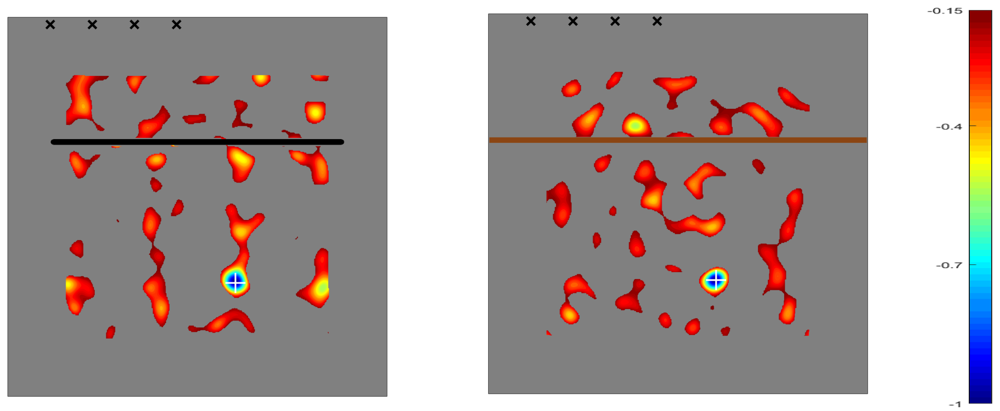
• Rectangular plates with constant thickness, but exhibiting either (i) an elongate through slit or (ii) an elongated inclusion of a different material, such as Titanium. Note that, in case (i), the through slit does not permit any transmission of the waves through it. Thus, the elongated slit cannot go from side to side transversally to the plate but should leave free portions of the plate at both sides of the slit. In case (ii), instead, the elongated inclusion permits partial transmission of the waves; thus, it can completely cover a section in the plate, from side to side. The elongated inclusion somewhat mimics the effect of stringers in the outer surface of aircraft wings. This application of topological sensitivity was performed in Reference [43], where it was seen that the method identifies defects, even in cases in which all emitters and receivers are at one side of the elongated artifact, while the defects are located at the other side.
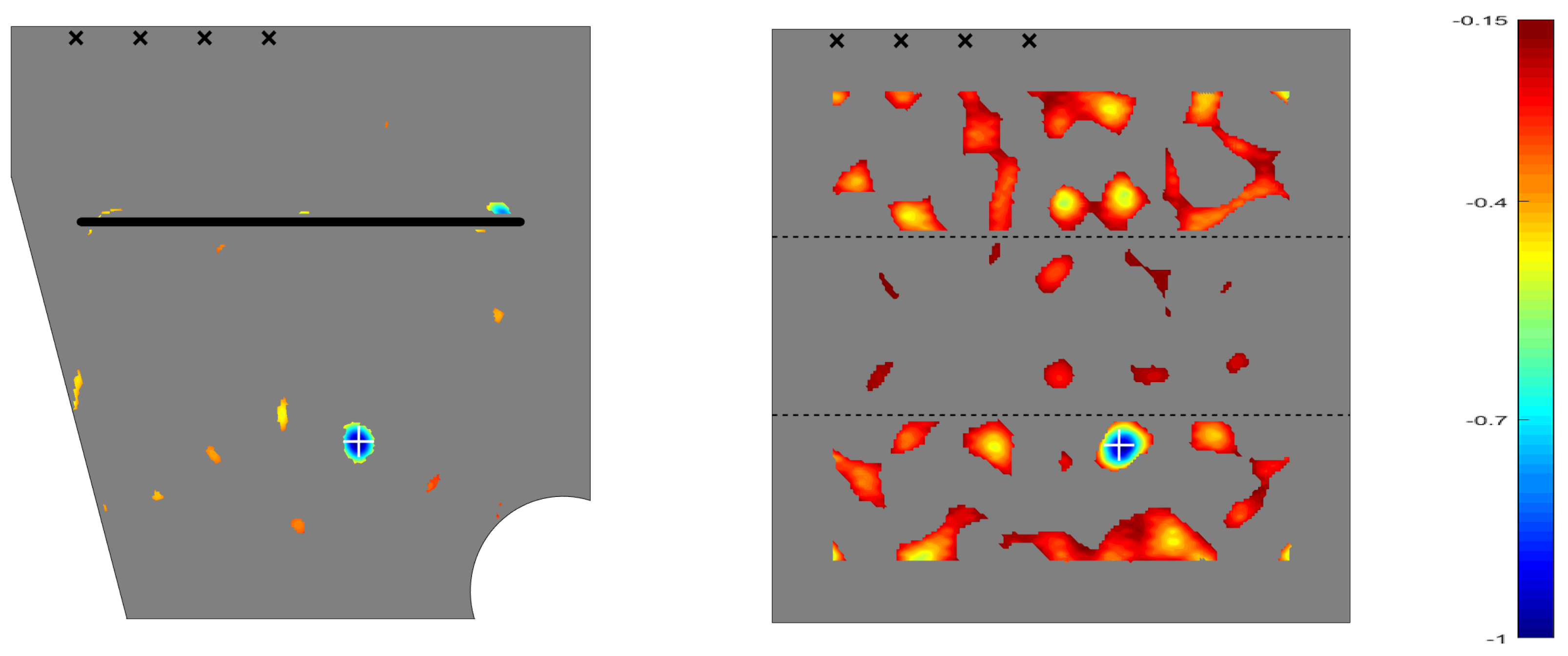
• Non-rectangular plates, exhibiting a complex planform or variable thickness. Difficulties for classical methods arise here from wave reflections in the boundaries and variable wave propagation speed (for guided waves) due to the variable thickness. This application was considered in Reference [44], where it was seen that, again, the method performs quite well.

These complex configurations cannot be efficiently analyzed using flight time-based classical methods. This is because, in the above mentioned cases, the through slit, the inclusion, or the limits of the sample induce a sudden (even infinite) jump in the acoustic impedance, producing a partial or total reflection of the wave that masks the reflections coming from the defects behind. The two above mentioned configurations are addressed below, one after another. In both cases, the set of emitters and sensors are either non-contact, optical laser devices [80], or contact piezo-electric, which may act as both emitters and receivers that operate as follows. Each time one of the devices acts as emitter, producing guided waves, the remaining devices act as receivers, sensing the incoming waves. A few dual devices will be used. These devices are located very close to the boundary of the plate planform, which makes the analysis more demanding but will use the possible (future) practical implementation of the method. In fact, locating these devices near the boundary highly worsens the performance of flight time-based classical methods. This is because the relevant outgoing (from emitters) and incoming (at the receivers) wave packets mix with their counterparts reflected at the nearby boundary, which distorts the relevant wave packets shape and, what is even worse, increases their thickness. Note that this decreases the accuracy in the computation of the flight time.

The topological sensitivity will not be computed in the whole plate but only in a slightly reduced in size interrogation window. This window is centered in the plate and excludes both a vicinity of the lateral boundary of the plate and the dual emitting/sensing devices themselves, to avoid misleading artifacts in the sensitivity that will appear due to the wave reflection at the lateral wall and the large values of the sensitivity near the emitting devices.

On the other hand, synthetic experimental data are used (obtained using an FEM solver), instead of actual experimental data. However, these synthetic data are calculated by solving the elastodynamic equations in a mesh that concentrates near the defects, while the mesh used in the computation of the direct and adjoint problems (needed to solve the inverse problem) is more equispaced, since the position and size of the defects are not known in the application of the method. In order to increase the amount of data collected in the sensors, the strategy developed in Reference [79] is used, in which the topological sensitivity-based method uses data obtained by considering a set of monochromatic excitations, with several (of the order of several tens) forcing frequencies of various amplitudes in the emitters.

Beginning with the case of a rectangular plate of constant thickness, but containing elongated slits or inclusions of a different material, two representative results, obtained upon application of the topological sensitivity method based on two-dimensional elastodynamics, are displayed in Figure 1, where the elongated artifacts, the emitters/receivers, and the defects are displayed. As can be seen in this figure, the dual emitting/sensing devices are located very close to the boundary of the plate planform, at the upper side of the elongated slit (which leaves a lateral portion of the plate free to allow wave propagation, as anticipated) or inclusion of a different material (which goes from side to side of the plate, as also anticipated), while the defect is located at the lower side. In spite of all these challenges, the method identifies the position of the defect fairly well, using 30 frequencies in the case with an elongated slit and 25 frequencies in the case of an elongated Titanium inclusion.

Turning now to the case in which the plate exhibits a complex planform or variable thickness, the outcome of the topological sensitivity method is given in Figure 2, where two representative cases are addressed, one with constant thickness but complex planform (which is addressed using two-dimensional elastodynamics) and the other with rectangular planform but variable thickness (which requires using three-dimensional elastodynamics). The complex planform configuration considered in the left plot contains a through slit to make the identification of the defect more demanding. The variable thickness plate, considered in the right plot, is thicker in the middle and thinner in the upper and lower sides of the plate. As in the cases considered in Figure 1, the emitting/receiving devices are located very close to a lateral boundary of the plate planform, and the method identifies well the small defect using 80 and 30 forcing frequencies in the cases considered in the left and right plots, respectively. Note that, in both cases, the emitting/receiving devices are at a different side of the through slit or plate thicker portion than that where the defect is.

Although, for simplicity in the presentation, all examples above are concerned with the simplest case in which a single defect is present, and the method can also cope with multiple defects of different sizes/shapes.

Thus, we can conclude that the topological sensitivity-based measurement post-processing method is a very promising tool to increase the defect detection threshold. The method is just an alternative way of analyzing data and very few modifications of existing experimental setups are needed, just to change the excitation signal from a chirp to several harmonic signals with different forcing frequencies. Additional details can be obtained from the authors.

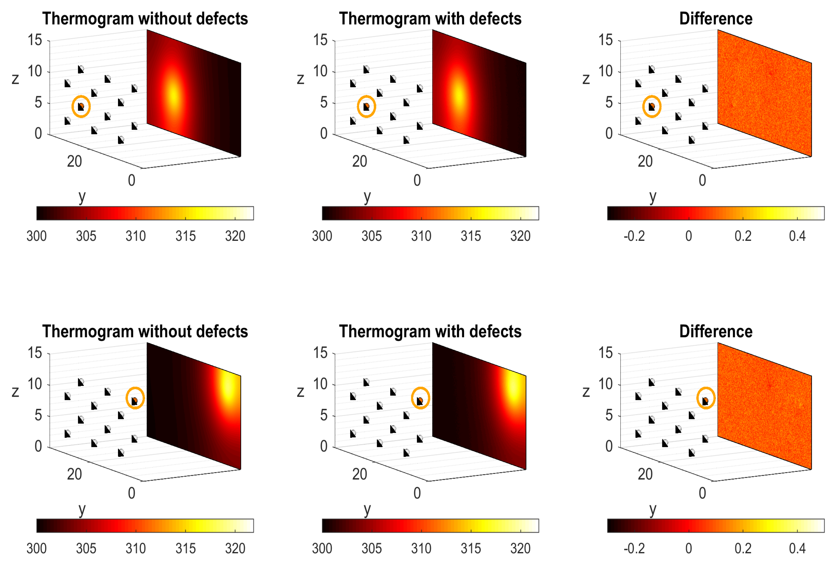
4. Application to SHM Using Infrared Thermography

Let us now consider the topological sensitivity approach for post-processing SHM data obtained via infrared (IR) active thermographic inspection. A topological sensitivity-based analysis using steady thermography was presented by us in Reference [81] (see Reference [82] for a preliminary theoretical analysis using steady thermograms, and also Reference [83] for an analysis using oscillatory, multifrequency, and thermograms) and had been already considered by other authors in References [84,85].

Steady thermograms produced in three-dimensional media obviously provide less information than dynamic thermograms. However, steady thermography can be more convenient, relevant, and beneficial in certain applications, such as medical tests for tumor detection [86] and in other areas of medical diagnosis [87].

As a general description of the technique, active thermographic inspection of a structure aims at recovering degradations in the structure properties (i.e., localized degradations of the density and thermal conductivity) from thermograms giving the temperature distribution in a part of the structure boundary, as resulting from the illumination using one or various lamps. In comparison with guided waves testing, IR testing has the advantage that it is more non-contact and non-invasive. However, heat transport is short range, and the associated signal-to-noise ratio is less favorable than its counterpart in elastic/acoustic wave propagation.

Concentrating, for simplicity in the exposition, on steady thermographic inspection of a rectangular plate, the governing Equation (9) is the conveniently discretized steady heat equation with appropriate boundary conditions. In this problem, the degradation vector $\tilde{\alpha }$ is the thermal conductivity function (depending on spatial variables) corresponding to the inhomogeneties of the metallic plate; the state vector $\mathit{u}$ is the temperature field at the illuminated face of the plate. Thus, the topological sensitivity of the cost function defined in (5) measures the sensitivity to perturbations of the thermal conductivity in the bulk of a homogeneous aluminum plate, which is otherwise assumed constant in the whole domain. This direct problem does not depend on the density and, thus, only permits localizing degradations in the thermal conductivity, which decreases the performance of the method.

Results will be given on steady IR thermographic inspection using twelve lamps contained in a $y-z$ plane, parallel to the cross section of the plate, in a Cartesian coordinate system (see Figure 3). These twelve lamps steadily illuminate, one after another (waiting for the plate reaching a steady state each time), on one side of the plate. Twelve thermograms capture the temperature distribution at the same side of the plate, after the steady state is reached each time. Thus, the number of available data is increased in a way similar to that developed in Reference [79].

The cross section of the plate is a $35\times 15$ cm${}^2$ rectangle, and its thickness equals 0.5 cm. A sketch of both the lamp positions and the plate with six small defects (representing no more than 0.1% of the total volume) is given in Figure 3.

As can be seen, the lamps are located equispacedly in a plane parallel to the plate planform, and the defects are much smaller than the transversal section of the plate.

In order to somehow mimic real experimental measurements, some random noise of size 0.05 K (which is larger than the expected error in experimental thermograms) has been added to the synthetic thermograms that are used here. The effect of the defects on the obtained thermograms is given in Figure 4.

This figure shows that the raw thermograms do not capture at all the presence of the defects. The application of the topological sensitivity method, instead, produces topological sensitivities that do localize the position of the defects, as seen in Figure 5.

Where the sections of the three-dimensional topological sensitivity with three representative planes are given, note that the method identifies the transversal position of the defects quite well, in contrast to what happened with the thermograms plotted in Figure 4. It is important to note that the topological sensitivity is computed from just the solution of the unperturbed direct and adjoint problems. The information about the defects characteristics is only introduced through the measured thermograms. Due to the weaker influence of depth in the topological sensitivity as compared with that of position or size the depth of the deffects, the depth of the defects is not well identified by the topological sensitivity. In addition, treating steady thermograms exhibits two drawbacks in connection with its practical use:

• Precise modeling of the process, which is needed to solve the direct and adjoint problems, is problematic, specially in connection with modeling the lamps energy deposition.
• Experimental steady thermograms are difficult to obtain, specially due to the large thermal relaxation time needed to reach each steady state.

It is because of the second difficulty that thermographic inspection in SHM is usually performed experimentally in highly unsteady conditions. Specifically, unsteady thermograms are recorded after illuminating one side of the plate by a quite short (of the order of ms) flash from the lamp. In this case, the thermal relaxation process towards the ambient temperature is recorded by the thermographic camera. In other words, this relaxation process can be modeled by the unsteady, unforced, homogeneous heat equation with initial conditions corresponding to the thermal state of the plate just after the flash. Moreover, in such thermal relaxation process, the instantaneous temperature in the unsteady termograms (computed at the plane illuminated by the lamp flash) can be written as

$$\theta (y,z,t)=\sum _{n=1}^N{\Theta }_n(y,z){\mathrm{e}}^{-{\delta }_{n}t},$$

(22)

where ${\Theta }_n(y,z)$ correspond to decaying natural modes of the homogeneous heat equation, and ${\delta }_n$ are the associated damping rates. Moreover, the modes and damping rates can be identified using a convenient data processing tool to the decaying thermograms. A good candidate tool to process these data is the recently developed higher order dynamic mode decomposition [88] (also see Reference [89] for a reader-friendly presentation of the method and its multiple applications), which is a very robust extension of standard dynamic mode decomposition [90,91]. Once the modes and damping rates have been identified, these permit applying a topological sensitivity approach in which the direct problem is robustly modeled by a Helmholtz-like equation associated with the homogeneous heat equation that applies here; the adjoint problem is modeled by the same Helmholtz-like equation, forced by the obtained modes ${\Theta }_n$, displayed in (22). This approach for solving the problem is in progress; thus, it is well beyond the scope of this review.

5. On Inverse Problems Associated with Diagnosis/Prognosis of Engineering Devices

Diagnosis and prognosis are concepts that arised in the medical field, in which diagnosis stands for identifying a present disease or illness in a patient [92] using symptoms, while prognosis [93] consists of predicting the likely future evolution of the diagnosed disease or illness, which intends determining a good present medical treatment to allow for a good evolution of the illness. These concepts have been extended to the technological field to, e.g., first performing diagnosis (which involves solving an inverse problem) in an engineering device, such as an aeroengine [94], and then using this to apply prognosis, which permits anticipating future failures in the device. The latter is known in the field as predictive maintenance [95], which anticipates failures, saving cost and time in the needed maintenance of the device.

Concentrating in diagnosis of an aeroengine, a detailed model for the system behavior is not possible. This is because such detailed model should account for the various, extremely complex, fluid dynamic, chemical, thermal, and elastic physical processes occurring inside the engine. Thus, a black-box model for the engine operation must be used to obtain the outcome of the direct problem, as formulated in (1). There are several black-box models in the field, which are based on phenomenological descriptions of the main engine subsystems (e.g., the fan and the low and high pressure compressors and turbines) that give very good results. One such model is built using commercial software [96]. Thus, the simplest formulation of the inverse problem described in Section 2 must be applied, in which the outcome of the direct problem is written according to Equation (1), which as explained in Section 2, requires that the sizes of the sensor and degradation vectors be both moderate. Fortunately enough, the number of components in the degradation vector is typically of the order of 10 components in the case of an aeroengine. Thus, the black-box solver can be used to solve problem (1), and the counterpart of the objective function (5) minimized, which has been done in Reference [97]. Following the idea developed in Reference [79] to increase the amount of available data, sensor measurements at two flight conditions are used, which multiplies by two the amount of available data. In addition, it must be taken into account that, in an aeroengine, the sensors outcomes account for various temperatures (measured in K), pressures (measured in Pa), rotational velocities (measured in rpm), and flow rates (measured in kg/s), which exhibit very disparate values, namely up to five orders of magnitude apart from one another. Thus, a convenient scaling of the sensors outcomes is a must. Let us note here that scaling is often quite important in optimization processes [76,77]. Still, flight conditions can only be ‘measured’ (in fact, estimated) in practice with low accuracy, which means that their precise values must be calculated, along with the degradations, when solving the inverse problem by minimizing the objective function.

Using an obvious (somewhat simple) scaling, the minimization of the objective function (to compute the degradations and the associated flight conditions) was performed in Reference [97], obtaining reasonably good results. However, the aforementioned optimization process was quite computationally expensive (requiring several CPU hours in a standard PC) because the Hessian of the objective function is quite ill-conditioned, which was to be expected, as anticipated in Section 2.

More recently, such large CPU time has been highly decreased (to a few CPU minutes) in Reference [98], where a suitable, somewhat subtle scaling of the sensor outcomes is performed. Moreover, the counterpart of the topological sensitivity (as defined in (7)) approach, gives very good results when degradations are very small, which is the usual case except if some important problem is occurring in the engine. The latter approximation gives good results requiring a very small CPU time, of the order of $0.01$ s, which is convenient to perform diagnosis in real time.

The application mentioned in this section is representative of diagnosis in realistic engineering systems considering this task as an inverse problem. In particular, a black-box solver must be usually employed since a detailed solver is not possible in these complex systems. However, using a black-box solver is possible since the size of the degradation vector is usually moderate. Finally, appropriate scaling of the data is a crucial step.

6. Conclusions

A general description, in mathematical terms, of the nature of inverse problems was given in Section 2, where two different cases were considered, one in which the number of degradations that need to be computed to define the health of the system is moderate, and another in which this number is extreamly large. Various strategies were presented to solve the inverse problem, including the topological sensitivity approach, which is the main object of this review. This method was used in Section 3 and Section 4 to address the associated inverse problem in SHM, considering both guided waves and themographic inspection, respectively, which give promising results in both cases.

In the case of ultrasound sensing, the topological sensitivity-based method has shown to be able to identify the position of small defects in very demanding cases, including rectangular plates with through slits or elongated inclusions of a different material, plates with more complex, non-rectangular planforms, and plates with variable thickness. In these cases, classical methods cannot give good results at all because of signal reflection at the boundaries or non-constant wave propagation velocity.

For thermographic analysis, steady thermography has proven, when combined with different heating combinations, capable of detecting the position and mesauring the size of defects. An extension of the method for unsteady thermography is expected to be able also to correctly predict the depth at which the defects are located.

Finally, diagnosis of engineering systems, considering this task as solving an inverse problem, was briefly addressed in Section 5, considering diagnosis of an aeroengine as test case to illustrate the application of the methods anticipated in Section 2.

Summarizing, the topological sensitivity approach has shown to be a very powerful tool for processing the adquired signals, with very different diagnosis techniques, allowing for the analysis of problems with very low signal-to-noise ratio.

References

1. Kac, M. Can one hear the shape of a drum? Am. Math. Mon. 1966, 73, 1–23. [Google Scholar] [CrossRef]
2. Protter, M.H. Can one hear the shape of a drum? revisited. SIAM Rev. 1987, 29, 185–197. [Google Scholar] [CrossRef]
3. Balageas, D.; Fritzen, C.P.; Güemes, J.A. Structural Health Monitoring; Wiley: Newport Beach, CA, USA; London, UK, 2010. [Google Scholar]
4. Carpio, A.; Rapún, M.-L. Solving inhomogeneous inverse problems by topological derivative methods. Inverse Probl. 2008, 24, 045014. [Google Scholar] [CrossRef]
5. Le Louër, F.; Rapún, M.-L. Detection of multiple impedance obstacles by non-iterative topological gradient based methods. J. Comput. Phys. 2019, 388, 534–560. [Google Scholar] [CrossRef]
6. Le Louër, F.; Rapún, M.-L. Topological sensitivity for solving inverse multiple scattering problems in three-dimensional electromagnetism. Part I: One step method. SIAM J. Imaging Sci. 2017, 10, 1291–1321. [Google Scholar] [CrossRef]
7. Le Louër, F.; Rapún, M.-L. Topological sensitivity for solving inverse multiple scattering problems in three-dimensional electromagnetism. Part II: Iterative method. SIAM J. Imaging Sci. 2018, 11, 734–769. [Google Scholar] [CrossRef]
8. Larrabide, I.; Novotny, A.A.; Feijóo, R.A.; Taroco, E. A medical image enhancement algorithm based on topological derivative and anisotropic diffusion. In Proceedings of the XXVI Iberian Latin-American Congress on Comput, Methods in Engineering-CILAMCE Guarapari, Espirito Santo, Brazil, 19–21 October 2005; pp. 1–14. [Google Scholar]
9. Meju, M.A. Geoelectromagnetic exploration for natural resources: Models, case studies and challenges. Surv. Geophys. 2002, 23, 133–205. [Google Scholar] [CrossRef]
10. Scott, W.R.; Schroeder, C.T.; Martin, J.S.; Larson, G.D. Use of elastic waves for the detection of buried land mines. In Proceedings of the Geoscience and Remote Sensing Symposium, IGARSS′01, IEEE 2001 International, Sydney, Australia, 9–13 July 2001; Volume 3, pp. 1116–1118. [Google Scholar]
11. Wunsch, C. The Ocean Circulation Inverse Problem; Cambridge University Press: Cambridge, UK, 1996. [Google Scholar]
12. Su, Z.; Ye, L.; Lu, Y. Guided Lamb waves for identification of damage in composite structures: A review. J. Sound Vib. 2006, 295, 753–780. [Google Scholar] [CrossRef]
13. Yan, F.; Boyer, F.L.; Rose, J.L. Ultrasonic guided wave imaging techniques in structural health monitoring. J. Intell. Mater. Syst. Struct. 2010, 21, 377–384. [Google Scholar] [CrossRef]
14. Zhu, X.; Rizzo, P.; Marzani, A.; Bruck, J. Ultrasonic guided waves for nondestructive evaluation/structural health monitoring of trusses. Meas. Sci. Technol. 2010, 21, 045701. [Google Scholar] [CrossRef]
15. Eschenauer, H.A.; Kobelev, V.; Schumacher, A. Bubble method for topology and shape optimization of structures. Struct. Optim. 1994, 8, 42–51. [Google Scholar] [CrossRef]
16. Sokowloski, J.; Zochowski, A. On the topological derivative in shape optimization. SIAM J. Control Optim. 1999, 37, 1251–1272. [Google Scholar] [CrossRef] [Green Version]
17. Ammari, H.; Garnier, J.; Jugnon, V.; Kang, H. Stability and resolution analysis for a topological derivative based imaging functional. SIAM J. Control Optim. 2012, 50, 48–76. [Google Scholar] [CrossRef] [Green Version]
18. Carpio, A.; Johansson, B.T.; Rapún, M.-L. Determining planar multiple sound-soft obstacles from scattered acoustic fields. J. Math. Imaging Vis. 2010, 36, 185–199. [Google Scholar] [CrossRef]
19. Carpio, A.; Rapún, M.-L. Topological derivatives for shape reconstruction. In Inverse Problems and Imaging, Lecture Notes in Mathematics; Springer: Berlin, Germany, 2008; pp. 85–134. [Google Scholar]
20. Feijoo, G.R. A new method in inverse scattering based on the topological derivative. Inverse Probl. 2004, 20, 1819–1840. [Google Scholar] [CrossRef]
21. Guzina, B.B.; Bonnet, M. Small-inclusion asymptotic of misfit functionals for inverse problems in acoustics. Inverse Probl. 2006, 22, 1761–1785. [Google Scholar] [CrossRef]
22. Ammari, H.; Bretin, E.; Garnier, J.; Jing, W.; Kang, H.; Wahab, A. Localization, stability, and resolution of topological derivative based imaging functionals in elasticity. SIAM J. Imaging Sci. 2013, 50, 48–76. [Google Scholar]
23. Bellis, C.; Bonnet, M. A fem-based topological sensitivity approach for fast qualitative identification of buried cavities from elastodynamic overdetermined boundary data. Int. J. Solids Struct. 2010, 47, 1221–1242. [Google Scholar] [CrossRef] [Green Version]
24. Bonnet, M.; Guzina, B.B. Sounding of finite solid bodies by way of topological derivative. Int. J. Numer. Meth. Eng. 2004, 61, 2344–2373. [Google Scholar] [CrossRef] [Green Version]
25. Guzina, B.B.; Bonnet, M. Topological derivative for the inverse scattering of elastic waves. Q. J. Mech. Appl. Math. 2004, 57, 161–179. [Google Scholar] [CrossRef] [Green Version]
26. Guzina, B.B.; Chikichev, I. From imaging to material identification: A generalized concept of topological sensitivity. J. Mech. Phys. Solids 2007, 55, 245–279. [Google Scholar] [CrossRef]
27. Oberai, A.A.; Gokhale, N.H.; Feijoo, G.R. Solution of inverse problems in elasticity imaging using the adjoint method. Inverse Probl. 2003, 19, 297–313. [Google Scholar] [CrossRef]
28. Carpio, A.; Rapún, M.-L. Domain reconstruction using photothermal techniques. J. Comput. Phys. 2008, 227, 8083–8106. [Google Scholar]
29. Carpio, A.; Rapún, M.-L. Parameter identification in photothermal imaging. J. Math. Imaging Vis. 2014, 49, 273–288. [Google Scholar] [CrossRef]
30. Carpio, A.; Rapún, M.-L. Hybrid topological derivative and gradient-based methods for electrical impedance tomography. Inverse Probl. 2012, 28, 095010. [Google Scholar] [CrossRef]
31. Carpio, A.; Rapún, M.-L. Hybrid topological derivative-gradient based methods for nondestructive testing. Abstr. Appl. Anal. 2013, 2013, 816134. [Google Scholar] [CrossRef]
32. Chaabane, S.; Masmoudi, M.; Meftahi, H. Topological and shape gradient strategy for solving geometrical inverse problems. J. Math. Anal. Appl. 2013, 400, 724–742. [Google Scholar] [CrossRef]
33. Ferreira, A.D.; Novotny, A.A. A new non-iterative reconstruction method for the electrical impedance tomography problem. Inverse Probl. 2017, 33, 035005. [Google Scholar] [CrossRef]
34. Hintermüller, M.; Laurain, A. Electrical impedance tomography: From topology to shape. Control Cybern. 2008, 37, 913–933. [Google Scholar]
35. Ahn, C.Y.; Jeon, K.; Ma, Y.-K.; Park, W.-K. A study on the topological derivative-based imaging of thin electromagnetic inhomogeneities in limited-aperture problems. Inverse Probl. 2004, 30, 105004. [Google Scholar] [CrossRef]
36. Masmoudi, M.; Pommier, J.; Samet, B. The topological asymptotic expansion for the Maxwell equations and some applications. Inverse Probl. 2005, 21, 547–564. [Google Scholar] [CrossRef]
37. Park, W.-K. Topological derivative strategy for one-step iteration imaging of arbitrary shaped thin, curve-like electromagnetic inclusions. J. Comput. Phys. 2012, 231, 1426–1439. [Google Scholar] [CrossRef]
38. Wahab, A. Stability and resolution analysis of topological derivative based localization of small electromagnetic inclusions. SIAM J. Imaging Sci. 2015, 8, 1687–1717. [Google Scholar] [CrossRef] [Green Version]
39. Wahab, A.; Abbas, T.; Ahmed, N.; Zia, Q.M.Z. Detection of electromagnetic inclusions using topological sensitivity. J. Comput. Math. 2017, 35, 642–671. [Google Scholar] [CrossRef] [Green Version]
40. Carpio, A.; Dimiduk, T.G.; Rapún, M.-L.; Selgas, V. Noninvasive imaging of three-dimensional micro and nanostructures by topological methods. SIAM J. Imaging Sci. 2016, 9, 1324–1354. [Google Scholar] [CrossRef] [Green Version]
41. Carpio, A.; Dimiduk, T.G.; Le Louër, F.; Rapún, M.-L. When topological derivatives met regularized Gauss-Newton iterations in holographic 3D imaging. J. Comput. Phys. 2019, 388, 224–251. [Google Scholar] [CrossRef] [Green Version]
42. Novotny, A.A.; Sokolowski, J.; Zochowski, A. Topological derivatives of shape functionals. Part II: First-order method and applications. J. Optim. Theory Appl. 2019, 180, 683–710. [Google Scholar] [CrossRef]
43. Martinez, A.; Güemes, J.A.; Perales, J.M.; Vega, J.M. SHM via topological derivative. Smart Mater. Struct. 2018, 27, 085002. [Google Scholar]
44. Martinez, A.; Güemes, J.A.; Perales, J.M.; Vega, J.M. Variable thickness in plates: A solution for SHM based on the topological derivative. Sensors 2020, 20, 2529. [Google Scholar] [CrossRef]
45. Aubert, G.; Drogoul, A. Topological gradient for fourth-order PDE and application to the detection of fine structures in 2D images. R. Acad. Sci. Paris 2014, 352, 609–613. [Google Scholar] [CrossRef] [Green Version]
46. Dominguez, N.; Gibiat, N. Non-destructive imaging using the time domain topological energy method. Ultrasonics 2010, 50, 367–372. [Google Scholar] [CrossRef] [PubMed]
47. Tokmashev, R. Experimental Validation of the Topological Sensitivity Approach to Elastic-Wave Imaging. Ph.D. Thesis, University of Minnesota, Minneapolis, MN, USA, 2015. [Google Scholar]
48. Tokmashev, R.; Tixier, A.; Guzina, B.B. Experimental validation of the topological sensitivity approach to elastic-wave imaging. Inverse Probl. 2013, 29, 125005. [Google Scholar] [CrossRef]
49. Xavier, M.; Fancello, E.A.; Farias, J.M.C.; Van Goethem, N.; Novotny, A.A. Topological derivative-based fracture modelling in brittle materials: A phenomenological approach. Eng. Fract. Mech. 2017, 179, 13–27. [Google Scholar] [CrossRef]
50. Yuang, H.; Guzina, B.B.; Chen, S.; Kinnick, R.; Fatemi, M. Application of topological sensitivity toward soft-tissue characterization from vibroacoustography measurements. J. Comput. Nonlinear Dyn. 2013, 8, 034503. [Google Scholar] [CrossRef]
51. Rodriguez, S.; Veidt, M.; Castaings, M.; Ducasse, E.; Deschamps, M. One channel defect imaging in a reverberating medium. Appl. Phys. Lett. 2014, 105, 1–5. [Google Scholar] [CrossRef] [Green Version]
52. Metwally, K.; Lubeigt, E.; Rakotonarivo, S.; Chaix, J.F.; Baqué, F.; Gobillot, G.; Mensah, S. Weld inspection by focused adjoint method. Ultrasonics 2018, 83, 80–88. [Google Scholar] [CrossRef]
53. Ben Hassen, M.F.; Erhard, K.; Potthast, R. The point-source method for 3D reconstructions for the Helmholtz equation and Maxwell equations. Inverse Probl. 2006, 22, 331–353. [Google Scholar] [CrossRef]
54. Cakoni, F.; Colton, D. Qualitative Methods in Inverse Scattering Theory: An Introduction; Springer: Berlin/Heidelberg, Germany, 2005. [Google Scholar]
55. Colton, D.; Kirsch, A. A simple method for solving inverse scattering problems in the resonance region. Inverse Probl. 1996, 12, 383–393. [Google Scholar] [CrossRef]
56. Ikehata, M. Reconstruction of an obstacle from the scattering amplitude at a fixed frequency. Inverse Probl. 1998, 14, 949–954. [Google Scholar] [CrossRef]
57. Kirsch, A. Characterization of the shape of a scattering obstacle using the spectral data of the far field operator. Inverse Probl. 1998, 14, 1489–1512. [Google Scholar] [CrossRef]
58. Kirsch, A. The music algorithm and the factorization method in inverse scattering theory for inhomogeneous media. Inverse Probl. 2002, 18, 1025–1040. [Google Scholar] [CrossRef]
59. Potthast, R. Stability estimates and reconstructions in inverse acoustic scattering using singular sources. J. Comput. Appl. Math. 2000, 114, 247–274. [Google Scholar] [CrossRef] [Green Version]
60. Potthast, R. A study on orthogonality sampling. Inverse Probl. 2010, 26, 074015. [Google Scholar] [CrossRef]
61. Dorn, O.; Lesselier, D. Level set methods for inverse scattering. Inverse Probl. 2006, 22, R67–R131. [Google Scholar] [CrossRef] [Green Version]
62. Harbrecht, H.; Hohage, T. Fast methods for three-dimensional inverse obstacle scattering problems. J. Integral Equ. Appl. 2007, 19, 237–260. [Google Scholar] [CrossRef]
63. Hettlich, F. Frechét derivatives in inverse obstacle scattering. Inverse Probl. 1995, 11, 371–382. [Google Scholar] [CrossRef]
64. Ivanyshyn Yaman, O.; Le Louër, F. Material derivatives of boundary integral operators in electromagnetism and application to inverse scattering problems. Inverse Probl. 2016, 32, 095003. [Google Scholar] [CrossRef] [Green Version]
65. Kirsch, A. The domain derivative and two applications in inverse scattering theory. Inverse Probl. 1993, 9, 81–96. [Google Scholar] [CrossRef]
66. Kress, R. Newton’s method for inverse obstacle scattering meets the method of least squares. Inverse Probl. 2003, 19, 91–104. [Google Scholar] [CrossRef]
67. Kress, R.; Rundell, W. A quasi-Newton method in inverse obstacle scattering. Inverse Probl. 1994, 10, 1145–1157. [Google Scholar] [CrossRef]
68. Ferreira de Rezende, S.W.; Vieira de Moura, J.; Mendes Finzi Neto, R.; Gallo, C.A.; Steffen, V. Convolutional neural network and impedance-based SHM applied to damage detection. Eng. Res. Express 2020, 2, 035031. [Google Scholar] [CrossRef]
69. Selva, P.; Cherrier, O.; Budinger, V.; Lachaud, F.; Morlier, J. Smart monitoring of aeronautical composites plates based on electromechanical impedance measurements and artificial neural network. Eng. Struct. 2013, 56, 794–804. [Google Scholar] [CrossRef] [Green Version]
70. Sepehry, N.; Shamshirsaz, M.; Abdollahi, F. Temperature variation effect compensation in impedance-based structural health monitoring using neural networks. J. Intell. Mater. Syst. Struct. 2011, 22, 1975–1982. [Google Scholar] [CrossRef]
71. Dung, C.V.; Anh, L.D. Autonomous concrete crack detection using deep fully convolutional neural network. Autom. Constr. 2019, 99, 52–58. [Google Scholar] [CrossRef]
72. Ebrahimkhanlou, A.; Salamonte, S. Single-sensor acoustic emission source location in plate-like structures using deep learning. Aerospacecraft 2018, 5, 50. [Google Scholar] [CrossRef] [Green Version]
73. Azimi, M.; Eslamlou, A.D.; Pekcan, G. Data-driven structural health monitoring and damage detection through deep learning: State-of-the-art review. Sensors 2020, 20, 2778. [Google Scholar] [CrossRef] [PubMed]
74. Yuan, F.-G.; Zargar, A.; Chen, K.; Wang, S. Machine learning for structural health monitoring: Challenges and opportunities. In Proceedings of the SPIE 11379, Sensors and Smart Structures Technologies for Civil, Mechanical, and Aerospace Systems 2020, Bellingham, WA, USA, 27 April–8 May 2020. [Google Scholar]
75. Seventekidis, P.; Giagopoulos, D.; Arailopous, A.; Markogiannaki, O. Structural health monitoring using deep learning with optimal finite element model generated data. Mech. Syst. Signal Process. 2020, 145, 106972. [Google Scholar] [CrossRef]
76. Fletcher, R. Practical Methods of Optimization; Wiley: Hoboken, NJ, USA, 1987. [Google Scholar]
77. Nocedal, J.; Wright, S.J. Numerical Optimization, 2nd ed.; Springer: New York, NY, USA, 2006. [Google Scholar]
78. Giles, M.B.; Pierce, N.A. An introduction to the adjoint approach to design. Flow Turbul. Combust. 2000, 65, 393–415. [Google Scholar] [CrossRef]
79. Funes, J.F.; Perales, J.M.; Rapún, M.-L.; Vega, J.M. Defect detection from multi-frequency limited data via topological sensitivity. J. Math. Imaging Vis. 2016, 55, 19–35. [Google Scholar] [CrossRef]
80. Royer, D.; Noroy, M.H.; Fink, M. Optical generation and detection of elastic waves in solids. J. Phys. IV 1994, 4, 673–683. [Google Scholar] [CrossRef] [Green Version]
81. Higuera, M.; Perales, J.M.; Rapún, M.-L.; Vega, J.M. Solving inverse geometry heat conduction problems by postprocessing steady thermograms. Int. J. Heat Mass Transf. 2019, 143, 118490. [Google Scholar] [CrossRef]
82. Pena, M.; Rapún, M.-L. Detecting damage in thin plates by processing infrared thermographic data with topological derivatives. Adv. Math. Phys. 2019, 2019, 5494795. [Google Scholar] [CrossRef]
83. Pena, M.; Rapún, M.-L. Application of the topological derivative to post-processing infrared time-harmonic thermograms for defect detection. J. Math. Ind. 2020, 10, 4. [Google Scholar] [CrossRef] [Green Version]
84. Ciampa, F.; Mahmoodi, P.; Pinto, F.; Meo, M. Recent advances in active infrared thermography for non-destructive testing of aerospace components. Sensors 2018, 18, 609. [Google Scholar] [CrossRef] [PubMed] [Green Version]
85. Cramer, K.E.; Howell, P.A.; Syed, H.I. Quantitative thermal imaging of aircraft structures. Proc. SPIE Thermosense XVII 1995, 2473, 226232. [Google Scholar]
86. Kandlikar, S.G.; Perez-Raya, I.; Raghupathi, P.A.; Gonzalez-Hernandez, J.L.; Dabydeen, D.; Medeiros, L.; Phatak, P. Infrared imaging technology for breast cancer detection—Current status, protocols and new directions. Int. J. Heat Mass Transf. 2017, 108, 2303–2320. [Google Scholar] [CrossRef]
87. Ring, E.F.J.; Ammer, K. Infrared thermal imaging in medicine. Physiol. Meas. 2012, 33, R33–R46. [Google Scholar] [CrossRef] [PubMed]
88. Le Clainche, S.; Vega, J.M. Higher order dynamic mode decomposition. SIAM J. Appl. Dyn. Syst. 2017, 16, 882–925. [Google Scholar] [CrossRef] [Green Version]
89. Vega, J.M.; Le Clainche, S. Higher Order Dynamic Mode Decomposition and Its Applications; Academic Press Cambridge: Cambridge, MA, USA, 2020. [Google Scholar]
90. Schmid, P.J.; Sesterhenn, J.L. Dynamic Mode Decomposition of numerical and experimental data. In Proceedings of the American Physical Society, 61st APS Meeting, San Antonio, CA, USA, 23–25 November 2008; p. 208. [Google Scholar]
91. Schmid, P.J. Dynamic mode decomposition of numerical and experimental data. J. Fluid Mech. 2010, 656, 5–28. [Google Scholar] [CrossRef] [Green Version]
92. Song, Y. A review of developments of EEG-based automatic medical support systems for epilepsy diagnosis and seizure detection. J. Biomed. Sci. Eng. 2011, 4, 788–796. [Google Scholar] [CrossRef] [Green Version]
93. Garcia-Crespo, A.; Alonso-Hernandez, G.; Battistella, L.; Rodriguez-Gonzalez, A. Methods and models for diagnosis and prognosis in medical systems. Comput. Math. Meth. Med. 2013, 2013, 184257. [Google Scholar] [CrossRef] [PubMed]
94. Urban, L. Gas path analysis applied to turbine engine condition monitoring. J. Aircr. 1973, 10, 400–406. [Google Scholar] [CrossRef]
95. Goriveau, R.; Medjaher, K.; Zerhouni, N. From Prognostics and Health Systems Management to Predictive Maintenance 1: Monitoring and Prognostics; Wiley: Hoboken, NJ, USA, 2016. [Google Scholar]
96. EcosimPro Proosis. Available online: https://www.ecosimpro.com/ (accessed on 29 November 2020).
97. Sanchez de León, L.; Rodrigo, J.; Vega, J.M.; Montañés, J.L. Gradient-like minimization methods for aeroengines diagnosis and control. Proc. Inst. Mech. Eng. Part G J. Aerosp. Eng. 2020. [Google Scholar] [CrossRef]
98. Rodrigo, J.; Sánchez de León, L.; Montañés, J.L.; Vega, J.M. An efficient method for performing aeroengines diagnosis. Preprint 2020. submitted. [Google Scholar]
Figure 1. Color maps of the topological sensitivity along a rectangular interrogation window in a rectangular Aluminium plate containing a through slit (indicated with a horizontal black line in the left plot) and a through inclusion of Titanium (indicated with a horizontal brown line in the middle plot); both plots share the color scale for the topological derivative, given in the right plot. In both cases, four dual emitters/receivers are considered, in which their positions are indicated with black x symbols, and the actual position of the defect indicated by a white + symbol. As can be seen, the method identifies well the position of the defect at the blue (negative) peak of the topological sensitivity. Courtesy of Dr. Anxo Martinez.
Applsci 11 01341 g001
Figure 2. Counterpart of Figure 1, considering a plate with complex planform (left) and variable thickness (right). In the latter case, that portion of the plate exhibiting larger thickness is indicated as that between the two dashed horizontal lines. Courtesy of Dr. Anxo Martinez.
Applsci 11 01341 g002
Figure 3. Sketch showing the lamp positions and the plate (in which scale along the x axis in the plate is enlarged to facilitate visualization, since the plate is really thin), with six small internal defects (in green) included. The volume of these defects represent no more than 0.1% of the total volume of the plate.
Applsci 11 01341 g003
Figure 4. The thermograms obtained for two positions of the lamp (left and middle plots), as obtained in the clean plate (without defects) and in the plate with internal defects. The difference between both thermograms is also given in the right plots. In each plot, the active lamp is represented by an orange circle.
Applsci 11 01341 g004
Figure 5. Color maps for the sections of the topological sensitivity with the planes x = 0 (left), x = 0.25 (middle), and x = 0.5 (right). The actual positions of the defects are shown by the six elongated black boxes. Negative peaks of the topological sensitivity coincide with defects positions.
Applsci 11 01341 g005
Publisher’s Note: MDPI stays neutral with regard to jurisdictional claims in published maps and institutional affiliations.