Simulink Model of a Thermoelectric Generator for Vehicle Waste Heat Recovery

Featured Application

The work presented in this study can be used in the design and development process of thermoelectric generators for vehicle waste heat recovery.

Abstract

More than 50% of the energy released through combustion in the internal combustion engine (ICE) is rejected to the environment. Recovering only a part of this energy can significantly improve the overall use of resources and the economic efficiency of road transport. One solution to recoup a part of this otherwise wasted thermal energy is to use thermoelectric generator (TEG) modules for the conversion of heat directly into electricity. To aid in development of this technology, this effort covers the derivation of a respectively simple steady-state Simulink model that can be utilized to estimate and optimize TEG system performance for ICEs. The model was validated against experimental data found in literature utilizing water cooling for the cold side. Overall, relatively good agreement was found with the maximum error in generated power around 10%. Following, it was investigated whether air can be used as a cooling medium. It was established that, at the same temperature as the water (18.4 °C), a flow velocity of 13.1 m/s (or 47.2 km/h) is required to achieve a similar cold junction temperature and power output. Subsequently using the model with air cooling, the performance of a TEG installed on a heavy-duty vehicle traveling at 50, 80, 90, and 120 km/h under different ambient temperatures was analyzed. It was determined that both a lower temperature and a higher flow velocity can improve power output. A further increase of the power output requires a larger temperature gradient across the module, which can be achieved by a higher heat input on the hot side.

1. Introduction

With the advent of the internal combustion engine (ICE) in the late 19th century and its continued development during the 20th century, humankind has benefited greatly from its use for transportation. In fact, the 20th century can be defined in one word: “Mobility”; local, regional, national, and international mobility of goods, people, and ideas. However, owing to its construction and general operation, the ICE manages to only partially transform fuel chemical energy into mechanical work. This is illustrated by the thermal efficiency of modern ICEs that generally only reaches 40–45%. This respectively low value of energy conversion directly influences the economic efficiency of the road transport process. For example, a 40 t freight vehicle with a payload of 25 t operating with an ICE has an overall transport process efficiency equal to 17–18% [1]. Furthermore, since transportation has a significant influence in both national and global economies, increasing transport process efficiency can immediately reduce operating costs while additionally helping to decrease greenhouse gas emissions.

Most of the thermal energy of the ICE (approx. 30%) is lost through the high temperature combustion exhaust gases that are discharged directly into the atmosphere. Therefore, one solution to increase overall efficiency is to recover, at least a part of this significant heat loss to the environment. For this purpose, research has targeted the design, development, and implementation of thermoelectric generator modules for directly converting heat into electricity, which can then be used in hybrid power systems to increase vehicle efficiency. Thermoelectric devices are environmentally friendly and have numerous other advantages including the lack of moving parts, the conversion of thermal energy directly into electrical energy, high reliability, as well as low maintenance requirements. The main disadvantage of such devices is their low efficiency owing to the small dimensionless figure of merit ($\mathrm{Z}\overline{\mathrm{T}}$) values currently found in commercial devices. However, there are promising solutions for achieving higher $\mathrm{Z}\overline{\mathrm{T}}$ values even at low to mid temperatures (<150 °C) [2].

The research efforts focused on identifying the potential for converting thermal energy into electricity, through thermoelectric generator (TEG) systems of different configurations and sizes, installed on the engine’s exhaust path show that it is possible to obtain an electrical power output of approximately 200–1000 W, depending on vehicle type and operating conditions [3,4,5,6]. However, research has also shown that the vehicular use of TEG systems depends on driving conditions with negative effects found when conditions have a high changing frequency [7].

The development of numerical models investigating the efficient use of TEG systems centers mainly on: Operating temperatures, optimizing geometric dimensions [8], different materials in TEG construction [9], and design optimization of hot and cold side heat exchangers [10]. Furthermore, TEG system design focuses on the energetic efficiency of conductive and convective system types [11]. In this area, Fan et al. [12] proposed a numerical model to determine the optimum values for the thermocouple leg lengths and cross-sectional areas. Their analysis showed that, for given thermal boundary conditions, the maximum output power can be improved by optimizing the leg length or cross-sectional area. Other efforts by Yu et al. [13] developed a mathematical model to investigate the effects of different vehicle engine operating regimes (e.g., cold-start and different loads) on TEG performance. The major conclusion of their research was that TEG performance is influenced more by vehicle speed than by ambient temperature. Wang et al. [14] used a three-dimensional computational fluid dynamics simulation to analyze power output, temperature distribution, and pressure drop of a TEG system with different internal structures of the heat exchanger. Their model considered the coverage and placement of the thermoelectric modules on the heat exchanger surface. The primary outcome was that increasing the number of modules may eventually saturate the total power output. Du et al. [15] investigated the design of a cooling channel for a thermoelectric module using a CFD software program (Fluent). Their results showed that in general, the output power is higher when using liquid as cooling fluid compared to air.

The analysis of this literature shows that there is a wide variety of numerical models for TEG simulation with different types of sophistication. However, most models are usually only briefly presented, with little detailing of the underlying equations and of the implementation. Therefore, the aim of this study is to develop and validate a respectively simple steady-state Simulink model that can be utilized to estimate and optimize TEG system performance. The model is intended to aid in the design and development of thermal energy recovery systems for ICEs, but it can be applied in other areas as well. Employing the described model early in the design process can facilitate whether thermal energy recovery is feasible for the TEG system under specific operating conditions. Furthermore, the proposed Simulink model can be integrated into existing software solutions for the analysis of different energy sources and powertrains.

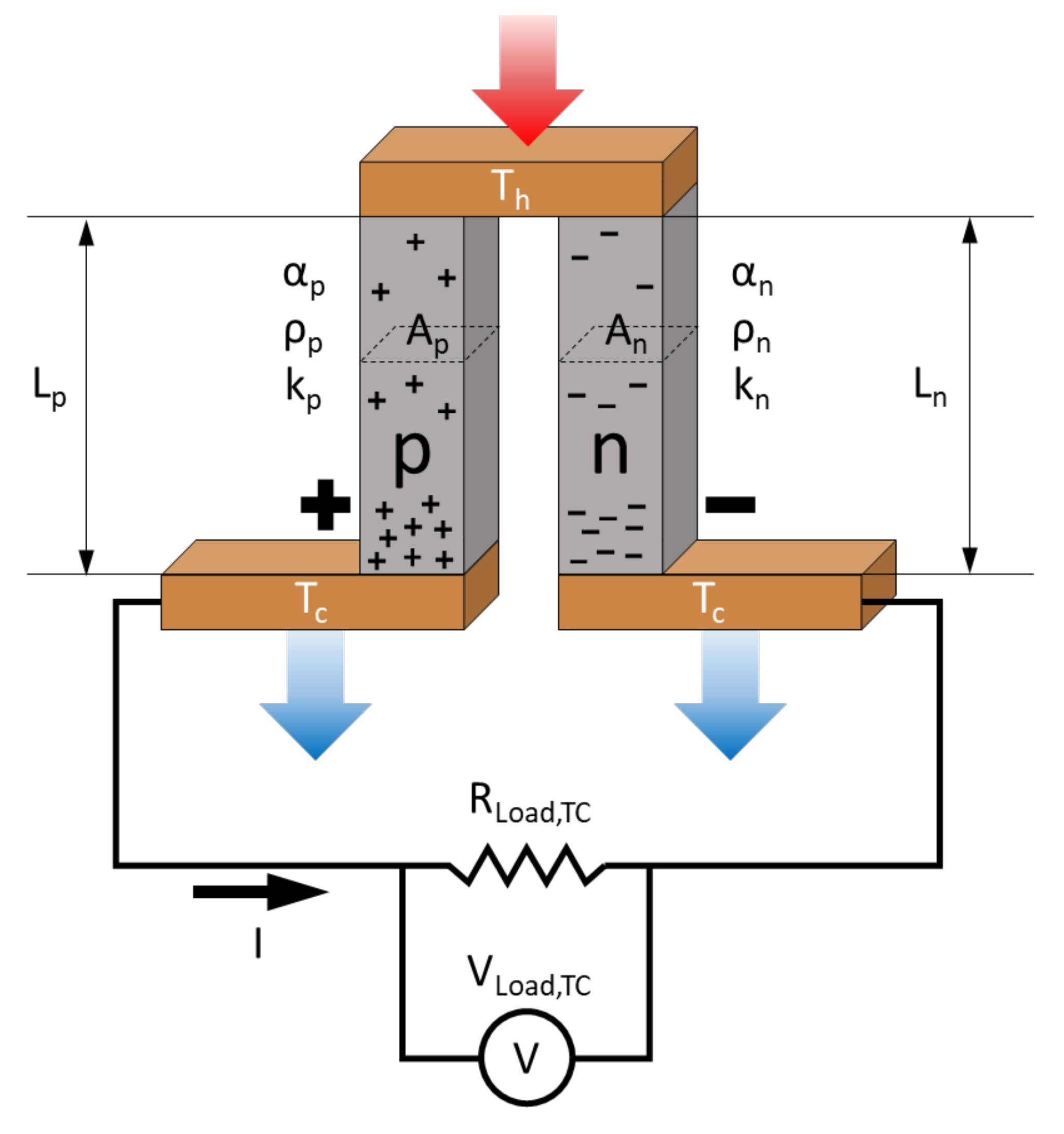
2. Thermoelectric Model Equations

A thermoelectric couple (TC) consists of p-type and n-type semiconductor legs that are connected thermally in parallel and electrically in series (Figure 1). When heat is applied to produce electric current, the TC operates as a generator. If, however, current is applied at the terminals, then the TC operates as a heat pump. For this effort, the focus is on thermoelectric generation and the use of the model as a heat pump is left to future work.

If the two junctions of the TC are subjected to different temperatures (ΔT = T_h − T_c [K], where T_h [K]—hot side temperature, T_c—cold side temperature), a potential difference, proportional to the temperature variation, will appear (V_OC,TC [V]—open circuit voltage, V_Load,TC [V]—potential difference across a load connected to the TC):

$${\mathrm{V}}_{\mathrm{O}\mathrm{C},\mathrm{T}\mathrm{C}}={\mathsf{\alpha }}_{\mathrm{T}\mathrm{C}}\cdot \left({\mathrm{T}}_{\mathrm{h}}-{\mathrm{T}}_{\mathrm{c}}\right)$$

(1)

where α_TC [V/K] is the relative Seebeck coefficient:

$${\mathsf{\alpha }}_{\mathrm{T}\mathrm{C}}={\mathsf{\alpha }}_{\mathrm{p}}-{\mathsf{\alpha }}_{\mathrm{n}}.$$

(2)

If the TC is connected to an external load with a resistance R_Load,TC [Ω], a current flow will appear (I [A]). Consequently, the potential difference V_Load,TC can be expressed as:

$${\mathrm{V}}_{\mathrm{L}\mathrm{o}\mathrm{a}\mathrm{d},\mathrm{T}\mathrm{C}}=\mathrm{I}\cdot {\mathrm{R}}_{\mathrm{L}\mathrm{o}\mathrm{a}\mathrm{d},\mathrm{T}\mathrm{C}}.$$

(3)

In addition, there is an internal electrical resistance of the TC, R_TC [Ω], which is defined based on the characteristics of the two legs: Electrical resistivity (ρ_p [Ωm]—electrical resistivity of the p-type leg, ρ_n [Ωm]—electrical resistivity of the n-type leg), length (L_p [m]—length of the p-type leg, L_n [m]—length of the n-type leg), and cross-sectional area (A_p [m²]—cross-section area of the p-type leg, A_n [m²]—cross-section area of the n-type leg).

$${\mathrm{R}}_{\mathrm{T}\mathrm{C}}={\mathsf{\rho }}_{\mathrm{p}}\frac{{\mathrm{L}}_{\mathrm{p}}}{{\mathrm{A}}_{\mathrm{p}}}+{\mathsf{\rho }}_{\mathrm{n}}\frac{{\mathrm{L}}_{\mathrm{n}}}{{\mathrm{A}}_{\mathrm{n}}}$$

(4)

Knowing that the relation between V_Load,TC and V_OC,TC is

$${\mathrm{V}}_{\mathrm{L}\mathrm{o}\mathrm{a}\mathrm{d},\mathrm{T}\mathrm{C}}={\mathrm{V}}_{\mathrm{O}\mathrm{C},\mathrm{T}\mathrm{C}}-\mathrm{I}{\mathrm{R}}_{\mathrm{T}\mathrm{C}}$$

(5)

which results in a derivation of the current:

$$\mathrm{I}=\frac{{\mathsf{\alpha }}_{\mathrm{T}\mathrm{C}}\left({\mathrm{T}}_{\mathrm{h}}-{\mathrm{T}}_{\mathrm{c}}\right)}{{\mathrm{R}}_{\mathrm{T}\mathrm{C}}+{\mathrm{R}}_{\mathrm{L}\mathrm{o}\mathrm{a}\mathrm{d},\mathrm{T}\mathrm{C}}}.$$

(6)

This flow of current leads to three additional effects: Peltier heating or cooling, Joule heating, and the Thomson effect. The latter is relatively small and is usually neglected to simplify the analysis, as is the case in this study.

If current flows through the junction, heat must be continuously added or rejected to maintain a constant temperature. Furthermore, this heat flow is proportional to the current flow and changes direction if the current is reversed. This is called the Peltier effect and is defined by the Peltier coefficient π_TC,junction [J/A]:

$${\mathsf{\pi }}_{\mathrm{T}\mathrm{C},\mathrm{j}\mathrm{u}\mathrm{n}\mathrm{c}\mathrm{t}\mathrm{i}\mathrm{o}\mathrm{n}}=\frac{{\dot{\mathrm{Q}}}_{\mathrm{j}\mathrm{u}\mathrm{n}\mathrm{c}\mathrm{t}\mathrm{i}\mathrm{o}\mathrm{n}}}{\mathrm{I}}$$

(7)

where $\dot{\mathrm{Q}}$_junction [W] is the rate of heat absorption/rejection at the hot/cold junction. Using Kelvin relationships, the Peltier coefficient can be expressed based on the Seebeck coefficient, which is respectively easier to measure:

$${\mathsf{\pi }}_{\mathrm{T}\mathrm{C},\mathrm{j}\mathrm{u}\mathrm{n}\mathrm{c}\mathrm{t}\mathrm{i}\mathrm{o}\mathrm{n}}={\mathsf{\alpha }}_{\mathrm{T}\mathrm{C}}{\mathrm{T}}_{\mathrm{j}\mathrm{u}\mathrm{n}\mathrm{c}\mathrm{t}\mathrm{i}\mathrm{o}\mathrm{n}}$$

(8)

where T_junction [K] is the temperature of the hot side and cold side junction. Thus, the rate of heat absorption/rejection at this junction can be expressed as:

$${\dot{\mathrm{Q}}}_{\mathrm{j}\mathrm{u}\mathrm{n}\mathrm{c}\mathrm{t}\mathrm{i}\mathrm{o}\mathrm{n}}={\mathsf{\alpha }}_{\mathrm{T}\mathrm{C}}\mathrm{I}{\mathrm{T}}_{\mathrm{j}\mathrm{u}\mathrm{n}\mathrm{c}\mathrm{t}\mathrm{i}\mathrm{o}\mathrm{n}}.$$

(9)

In addition to Joule heating, there is another irreversible phenomenon that accompanies the reversible thermoelectric effect, namely the conduction of heat. In a TC, heat conduction causes a transfer of heat from the hot side to the cold side as a means of achieving thermal equilibrium. Considering the thermal conductivities of the two legs (k_p [W/mK]—thermal conductivity of the p-type leg, k_n [W/mK]—thermal conductivity of the n-type leg), one can define the thermal conductance (K_TC [W/K]) of the TC:

$${\mathrm{K}}_{\mathrm{T}\mathrm{C}}={\mathrm{k}}_{\mathrm{p}}\frac{{\mathrm{A}}_{\mathrm{p}}}{{\mathrm{L}}_{\mathrm{p}}}+{\mathrm{k}}_{\mathrm{n}}\frac{{\mathrm{A}}_{\mathrm{n}}}{{\mathrm{L}}_{\mathrm{n}}}.$$

(10)

Joule heating, $\dot{\mathrm{Q}}$_Joule,h/c [W], is the process where electrical energy is converted into thermal energy as current flows through a resistance. For a TC, Joule heating decreases the rate of heat absorption at the hot junction and increases the rate of heat transfer to the cold junction, in equal shares (i.e., half of the heat generated by the Joule effect passes to the hot side and the other half to the cold side) [16]:

$${\dot{\mathrm{Q}}}_{\mathrm{J}\mathrm{o}\mathrm{u}\mathrm{l}\mathrm{e},\mathrm{h}/\mathrm{c}}=\frac{1}{2}{\mathrm{I}}^2{\mathrm{R}}_{\mathrm{T}\mathrm{C}}.$$

(11)

Neglecting the Thomson effect, by applying the first law of thermodynamics at the hot junction of a TC, the rate of heat absorption, $\dot{\mathrm{Q}}$_h,TC [W], is:

$${\dot{\mathrm{Q}}}_{\mathrm{h},\mathrm{T}\mathrm{C}}={\mathsf{\alpha }}_{\mathrm{T}\mathrm{C}}\mathrm{I}{\mathrm{T}}_{\mathrm{h}}-\frac{1}{2}{\mathrm{I}}^2{\mathrm{R}}_{\mathrm{T}\mathrm{C}}+{\mathrm{K}}_{\mathrm{T}\mathrm{C}}\left({\mathrm{T}}_{\mathrm{h}}-{\mathrm{T}}_{\mathrm{c}}\right)$$

(12)

whereas the rate of heat rejection, $\dot{\mathrm{Q}}$_c,TC [W], at the cold side is:

$${\dot{\mathrm{Q}}}_{\mathrm{c},\mathrm{T}\mathrm{C}}={\mathsf{\alpha }}_{\mathrm{T}\mathrm{C}}\mathrm{I}{\mathrm{T}}_{\mathrm{c}}+\frac{1}{2}{\mathrm{I}}^2{\mathrm{R}}_{\mathrm{T}\mathrm{C}}+{\mathrm{K}}_{\mathrm{T}\mathrm{C}}\left({\mathrm{T}}_{\mathrm{h}}-{\mathrm{T}}_{\mathrm{c}}\right).$$

(13)

Overall, the power delivered to the load, P_el,TC [W], can be calculated in two ways:

$${\mathrm{P}}_{\mathrm{e}\mathrm{l},\mathrm{T}\mathrm{C}}={\dot{\mathrm{Q}}}_{\mathrm{h},\mathrm{T}\mathrm{C}}-{\dot{\mathrm{Q}}}_{\mathrm{c},\mathrm{T}\mathrm{C}}$$

(14)

or as:

$${\mathrm{P}}_{\mathrm{e}\mathrm{l},\mathrm{T}\mathrm{C}}={\mathrm{I}}^2{\mathrm{R}}_{\mathrm{L}\mathrm{o}\mathrm{a}\mathrm{d},\mathrm{T}\mathrm{C}}.$$

(15)

The thermoelectric performance of the material is assessed using the figure of merit [1/K]:

$$\mathrm{Z}=\frac{{\mathsf{\alpha }}^2}{\mathsf{\rho }\mathrm{k}}$$

(16)

which, for a TC becomes

$${\mathrm{Z}}_{\mathrm{T}\mathrm{C}}=\frac{{\mathsf{\alpha }}_{\mathrm{T}\mathrm{C}}^2}{{\left[\sqrt{{\mathsf{\rho }}_{\mathrm{p}}{\mathrm{k}}_{\mathrm{p}}}+\sqrt{{\mathsf{\rho }}_{\mathrm{n}}{\mathrm{k}}_{\mathrm{n}}}\right]}^2}.$$

(17)

This figure of merit, like the thermoelectric parameters, is temperature dependent. However, often, average values are assumed with errors found to be below 10% of the true value [17].

The conversion (or thermal) efficiency of the TC is the ratio of the power output to the heat input at the hot side. To simplify the final expression, the following notations are employed for the load resistance ratio (m [-]) and Carnot efficiency (η_C [-]), respectively,

$$\mathrm{m}=\frac{{\mathrm{R}}_{\mathrm{L}\mathrm{o}\mathrm{a}\mathrm{d},\mathrm{T}\mathrm{C}}}{{\mathrm{R}}_{\mathrm{T}\mathrm{C}}}$$

(18)

$${\mathsf{\eta }}_{\mathrm{C}}=1-\frac{{\mathrm{T}}_{\mathrm{c}}}{{\mathrm{T}}_{\mathrm{h}}}.$$

(19)

Thus, the conversion efficiency is:

$${\mathsf{\eta }}_{\mathrm{t}\mathrm{h}}=\frac{{\mathsf{\eta }}_{\mathrm{C}}\mathrm{m}}{\left(1+\mathrm{m}\right)-\frac{1}{2}{\mathsf{\eta }}_{\mathrm{C}}+\frac{1}{2\mathrm{Z}\overline{\mathrm{T}}}{\left(1+\mathrm{m}\right)}^2\left(1+\frac{{\mathrm{T}}_{\mathrm{c}}}{{\mathrm{T}}_{\mathrm{h}}}\right)}.$$

(20)

Expressions of maximum parameters (current, voltage, power, and efficiency) are also introduced here due to their importance in determining TEG parameters, which will be shown later. The maximum voltage occurs at open circuit when I = 0:

$${\mathrm{V}}_{\mathrm{O}\mathrm{C},\mathrm{T}\mathrm{C},\max }={\mathsf{\alpha }}_{\mathrm{T}\mathrm{C}}\left({\mathrm{T}}_{\mathrm{h}}-{\mathrm{T}}_{\mathrm{c}}\right).$$

(21)

The maximum current, however, occurs at short circuit, where R_Load,TC = 0; thus, leading to the following expression:

$${\mathrm{I}}_{\max }=\frac{{\mathsf{\alpha }}_{\mathrm{T}\mathrm{C}}\left({\mathrm{T}}_{\mathrm{h}}-{\mathrm{T}}_{\mathrm{c}}\right)}{{\mathrm{R}}_{\mathrm{T}\mathrm{C}}}.$$

(22)

To obtain the maximum power, it can be shown that the load resistance must equal the internal resistance (thus: m = 1), which leads to the following expression:

$${\mathrm{P}}_{\mathrm{e}\mathrm{l},\max }=\frac{{\mathsf{\alpha }}_{\mathrm{T}\mathrm{C}}^2{\left({\mathrm{T}}_{\mathrm{h}}-{\mathrm{T}}_{\mathrm{c}}\right)}^2}{4{\mathrm{R}}_{\mathrm{T}\mathrm{C}}}$$

(23)

For the maximum efficiency, the conversion efficiency is differentiated with respect to m and set to 0. This leads to the following expression for the load resistance ratio:

$$\mathrm{m}=\sqrt{1+\mathrm{Z}\overline{\mathrm{T}}}$$

(24)

where $\mathrm{Z}\overline{\mathrm{T}}$ [-] is the dimensionless figure of merit ($\overline{\mathrm{T}}=1/2\cdot \left({\mathrm{T}}_{\mathrm{h}}+{\mathrm{T}}_{\mathrm{c}}\right)$ [K] is the average temperature across the TC). Consequently, the maximum conversion efficiency becomes:

$${\mathsf{\eta }}_{\mathrm{t}\mathrm{h},\max }=\left(1-\frac{{\mathrm{T}}_{\mathrm{c}}}{{\mathrm{T}}_{\mathrm{h}}}\right)\cdot \frac{\sqrt{1+\mathrm{Z}\overline{\mathrm{T}}}-1}{\sqrt{1+\mathrm{Z}\overline{\mathrm{T}}}+\frac{{\mathrm{T}}_{\mathrm{c}}}{{\mathrm{T}}_{\mathrm{h}}}}.$$

(25)

Of additional high importance is the efficiency at maximum power (η_mp), or, in other words, at matching load resistance (m = 1). Based on Equation (20), η_mp is:

$${\mathsf{\eta }}_{\mathrm{mp}}=\frac{{\mathsf{\eta }}_{\mathrm{C}}}{2-\frac{1}{2}{\mathsf{\eta }}_{\mathrm{C}}+\frac{2}{\mathrm{Z}\overline{\mathrm{T}}}\left(1+\frac{{\mathrm{T}}_{\mathrm{c}}}{{\mathrm{T}}_{\mathrm{h}}}\right)}.$$

(26)

The output of a single TC is generally small; e.g., well below 1 [W]. Therefore, many TCs are connected to form a thermoelectric module (TEM) (Figure 2); thus, increasing the power output. At this point it is worth recalling that a TEM can operate both as a generator (often designated with TEG in literature) and/or as a heat pump (usually TEC—thermoelectric cooler). In the present study, the TEM operates as a generator, but the notation of TEM is used to avoid confusion with the acronym TEG that involves the overall system including heat exchangers (shown later). The output of a TEM can be expressed based on the number of thermocouples (n_TC [-]) and the parameters of the TC, except for electrical current that is independent of the number of thermocouples. Thus, the total rate of heat absorption/rejection at the hot and cold sides are, respectively:

$${\dot{\mathrm{Q}}}_{\mathrm{h},\mathrm{T}\mathrm{E}\mathrm{M}}={\mathrm{n}}_{\mathrm{T}\mathrm{C}}\left[{\mathsf{\alpha }}_{\mathrm{T}\mathrm{C}}\mathrm{I}{\mathrm{T}}_{\mathrm{h}}-\frac{1}{2}{\mathrm{I}}^2{\mathrm{R}}_{\mathrm{T}\mathrm{C}}+{\mathrm{K}}_{\mathrm{T}\mathrm{C}}\left({\mathrm{T}}_{\mathrm{h}}-{\mathrm{T}}_{\mathrm{c}}\right)\right]$$

(27)

$${\dot{\mathrm{Q}}}_{\mathrm{c},\mathrm{T}\mathrm{E}\mathrm{M}}={\mathrm{n}}_{\mathrm{T}\mathrm{C}}\left[{\mathsf{\alpha }}_{\mathrm{T}\mathrm{C}}\mathrm{I}{\mathrm{T}}_{\mathrm{c}}+\frac{1}{2}{\mathrm{I}}^2{\mathrm{R}}_{\mathrm{T}\mathrm{C}}+{\mathrm{K}}_{\mathrm{T}\mathrm{C}}\left({\mathrm{T}}_{\mathrm{h}}-{\mathrm{T}}_{\mathrm{c}}\right)\right].$$

(28)

Using Equations (14), (27) and (28), the total power output of the module can be calculated:

$${\mathrm{P}}_{\mathrm{e}\mathrm{l},\mathrm{T}\mathrm{E}\mathrm{M}}={\mathrm{n}}_{\mathrm{T}\mathrm{C}}\left[{\mathsf{\alpha }}_{\mathrm{T}\mathrm{C}}\mathrm{I}\left({\mathrm{T}}_{\mathrm{h}}-{\mathrm{T}}_{\mathrm{c}}\right)-{\mathrm{I}}^2{\mathrm{R}}_{\mathrm{T}\mathrm{C}}\right].$$

(29)

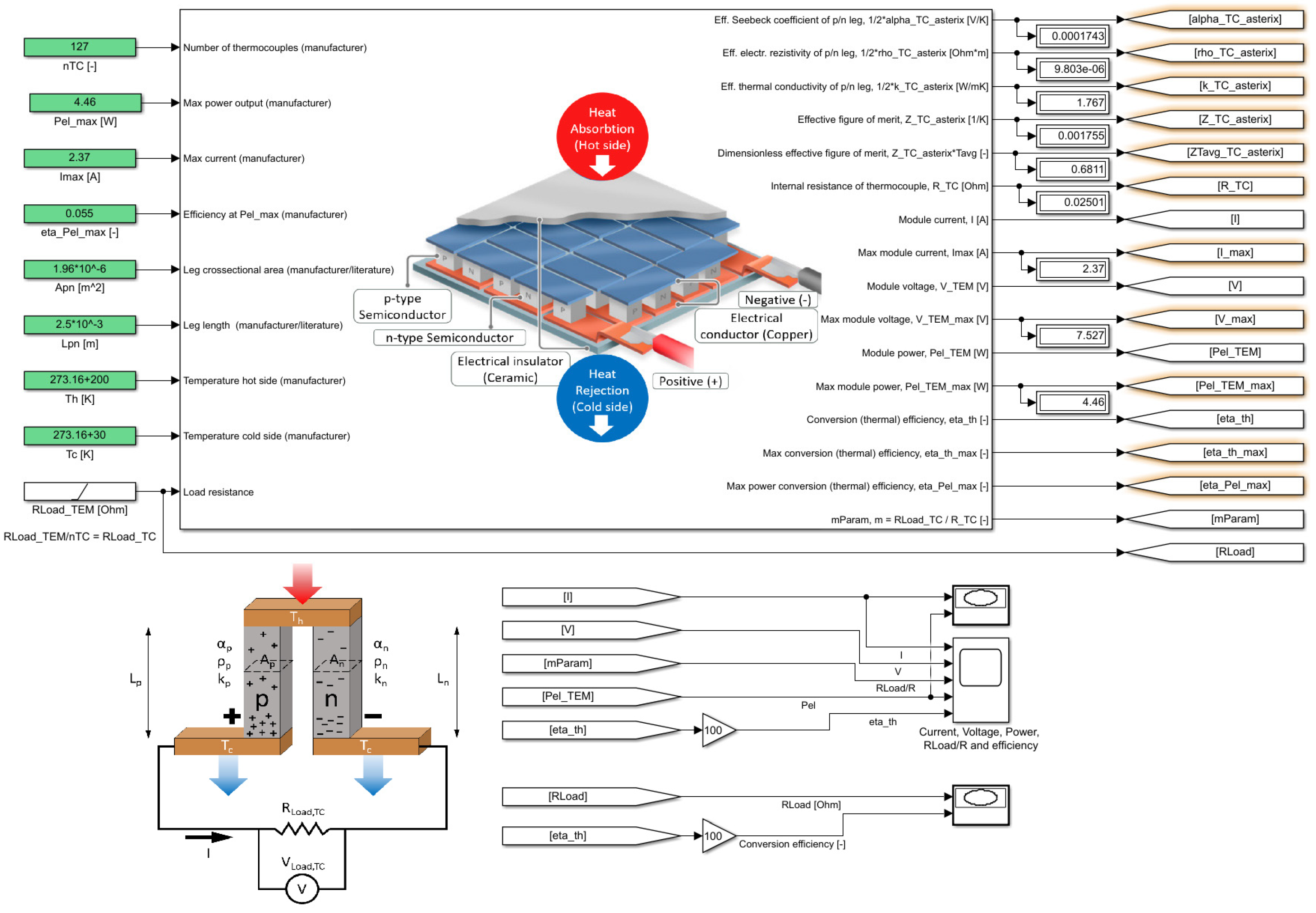
3. TEM Properties Identification Model

Often TEM material properties are not available from the manufacturer and must be determined, which requires specialized equipment [19]. Furthermore, it is not always necessary to have high model accuracy throughout the entire operating range. For example, when estimating the performance of a TEM system in the preliminary design phase, it is helpful to have a respectively simple and physically based model that can be used to run parametric studies. To solve this issue, Lee et al. [20] and Zhang [21] proposed methods that use maximum parameter values, usually provided by manufacturers, to estimate the electrical resistivity, Seebeck coefficient, thermal conductivity, and the figure of merit. The authors call these effective parameters since, as compared to intrinsic material properties, they are determined at the system (TEM) level; thus, they account for the various losses caused by the manufacturing process (i.e., thermal and electrical contact resistances), the temperature dependency (due to the Thomson effect), as well as imperfect insulation (heat losses through radiation and convection). The basic idea is that, ideally, the maximum current, voltage, power, and efficiency are functions of the material properties, the thermocouple geometry (area, length), and the temperatures of the two junctions (T_h, T_c).

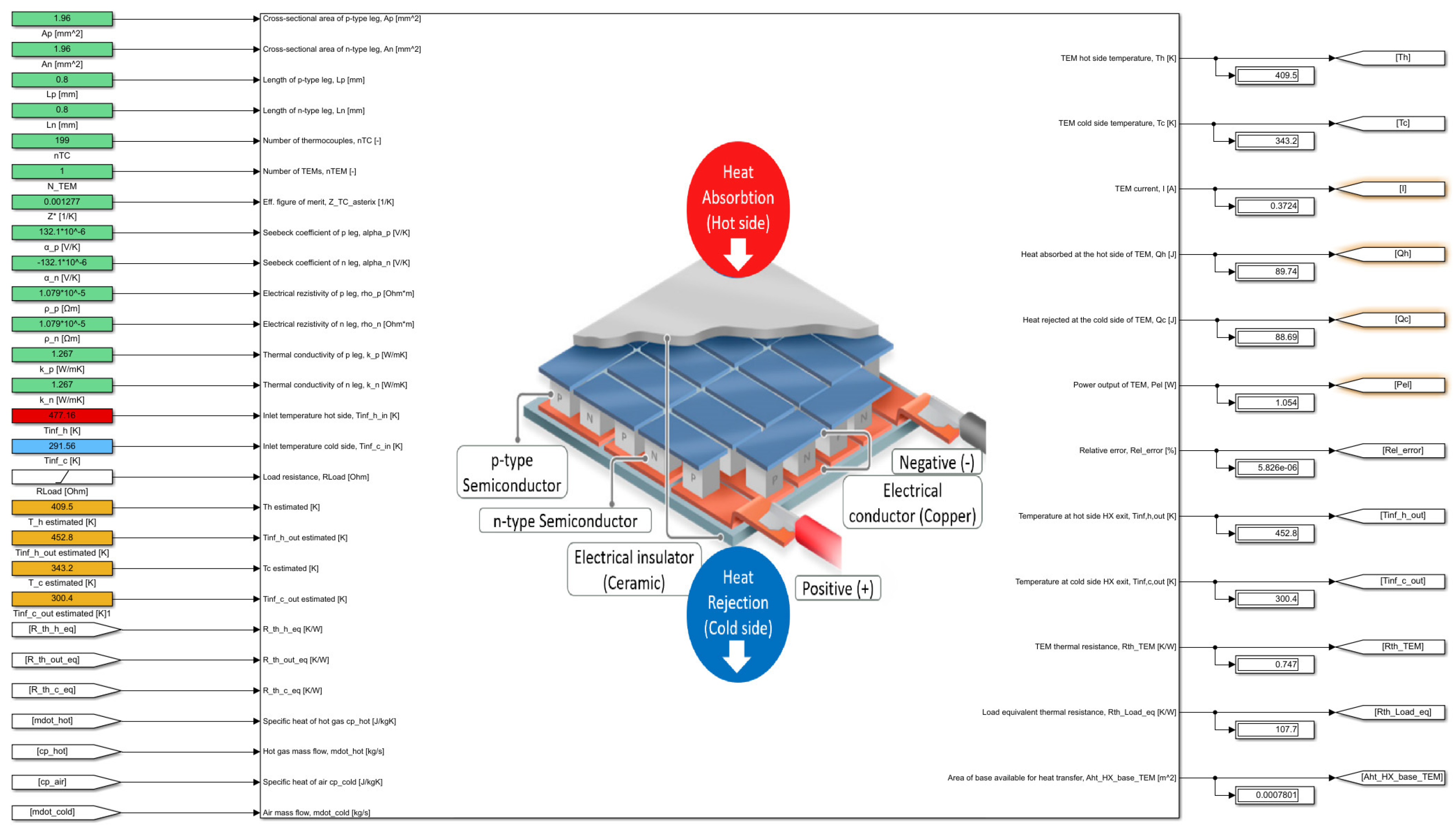
3.1. Equations and Simulink Model

For the current study, the maximum parameters used to determine the outcomes are current, efficiency, and power (only three of the four maximum parameters presented in Equations (21)–(23) and (25) are required). By knowing the leg area (A = A_p = A_n) and length (L = L_p = L_n), the effective Seebeck coefficient and the effective electrical resistivity of the TC can be determined from Equations (22) and (23):

$${\mathsf{\rho }}_{\mathrm{T}\mathrm{C}}^{\ast }=\frac{4\left(\frac{\mathrm{A}}{\mathrm{L}}\right){\mathrm{P}}_{\mathrm{e}\mathrm{l},\max }}{{\mathrm{n}}_{\mathrm{T}\mathrm{C}}{\mathrm{I}}_{\max }^2}$$

(30)

$${\mathsf{\alpha }}_{\mathrm{T}\mathrm{C}}^{\ast }=\frac{4{\mathrm{P}}_{\mathrm{e}\mathrm{l},\max }}{{\mathrm{n}}_{\mathrm{T}\mathrm{C}}{\mathrm{I}}_{\max }\left({\mathrm{T}}_{\mathrm{h}}-{\mathrm{T}}_{\mathrm{c}}\right)}.$$

(31)

To determine the effective thermal conductivity, an additional parameter is required, namely the effective figure of merit which can be obtained from Equation (25):

$${\mathrm{Z}}_{\mathrm{T}\mathrm{C}}^{\ast }=\frac{1}{\overline{\mathrm{T}}}\left[{\left(\frac{1+\frac{{\mathsf{\eta }}_{\max }}{{\mathsf{\eta }}_{\mathrm{C}}}\frac{{\mathrm{T}}_{\mathrm{c}}}{{\mathrm{T}}_{\mathrm{h}}}}{1-\frac{{\mathsf{\eta }}_{\max }}{{\mathsf{\eta }}_{\mathrm{C}}}}\right)}^2-1\right].$$

(32)

Based on Equation (16), the effective thermal conductivity can be expressed as:

$${\mathrm{k}}_{\mathrm{T}\mathrm{C}}^{\ast }=\frac{{\mathsf{\alpha }}_{\mathrm{T}\mathrm{C}}^{\ast }{}^2}{{\mathrm{Z}}_{\mathrm{T}\mathrm{C}}^{\ast }{\mathsf{\rho }}_{\mathrm{T}\mathrm{C}}^{\ast }}.$$

(33)

3.2. Model Validation

The model has been validated for two commercially available thermoelectric modules which are presented in

Table 1. Thermoelectric parameters of commercially available thermoelectric modules.

TEM	nTC [-]	Pel,max [W]	Imax [A]	ηmax [%]	Ap/n [mm2]	Lp/n [mm]	Th [°C]	Tc [°C]
TGM-199-1.4-0.8 [22]	199	11.40	5.10	4.3	1.96	0.8	200	30
TGM-127-1.4-2.5 [23]	127	4.46	2.37	5.5	1.96	2.5	200	30

. This data has been used in the Simulink model presented in Figure 3 to determine the effective parameters.

The effective parameters obtained with the model presented in Figure 3 were used to calculate the voltage, current, and power at matched load resistance conditions, as well as the power, current, voltage, and efficiency at the maximum temperature gradient for various values of the load resistance. The results show that there is a relatively good agreement between the measured and calculated values (Figure 4 and Figure 5). The major differences appearing here can be attributed to the temperature dependency of the electrical resistivity, Seebeck coefficient, and thermal conductivity, which is not captured in the proposed model. Despite these differences, the predicted power output of the module is in relatively good agreement with the measured values. A possible reason for this result is that the maximum power was chosen as an input parameter in deference to the maximum voltage.

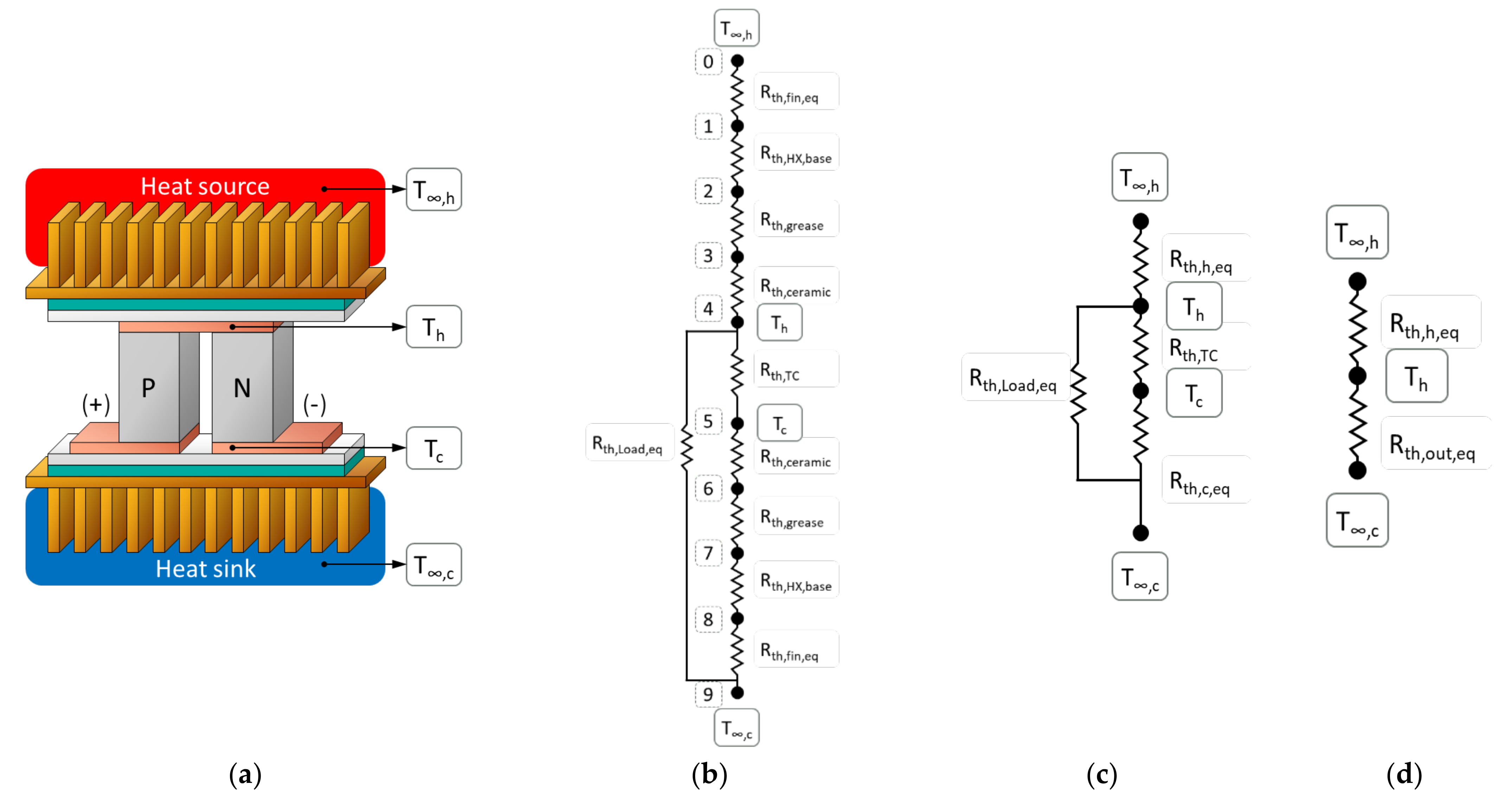
4. TEG Model for Exhaust Gas Waste Heat Recovery

For the current study, the system is analyzed under steady-state conditions. The domain is discretized along the flow direction in control volumes (CVs) having the same length as a TEM (Figure 6). Initially, only one control volume is considered for the calculation; however, a greater domain can be built by adding more control volumes with each taking input data from the previous CV. The changes in fluid properties with temperature are considered separately for each control volume and are defined at the mean CV temperature (average of inlet and outlet temperatures). For simplicity, thermoelectric parameters are considered constant, but the model can be readily updated with equations for these parameters, either from the literature or from the manufacturer.

Thermoelectric modules are often combined with heat exchangers (HX) to form thermoelectric generators (TEG), which are used to recover otherwise wasted thermal energy from the exhaust gases of ICEs. The fins of the HX allow for an increased heat transfer surface area, subsequently enhancing the amount of heat extracted through convection from the hot gases. This heat is then transferred through conduction to the TEMs. An example of such a TEG with all relevant dimensions of the finned heat exchanger (L_HX [m]—heat exchanger length, W_HX [m]—heat exchanger width, H_HX [m]—heat exchanger height, z_{HX,fin-spacing} [m]—heat exchanger fin spacing, t_HX,fin [m]—heat exchanger fin thickness), as well as the positioning of the TEMs is presented in Figure 6. If the heat exchanger is covered with TEMs on both sides, the CV must be modified accordingly (Figure 7).

4.1. Equations and Simulink Model

The layering of the TEG, which will be used for calculating the amount of heat transferred to the hot side and from the cold side, is presented in Figure 8. The TEG is composed of two heat exchangers (hot and cold side), a thermal grease used to eliminate surface imperfections in the interface area, and two ceramic plates acting as electric insulators. The electrical conductor height is relatively small and, since it has a respectively high thermal conductivity and low electrical resistivity, it was neglected in the present model.

As a first step, all relevant areas for the heat transfer are calculated starting from the area available for heat transfer in one TC (A_ht,TC [m²]):

$${\mathrm{A}}_{\mathrm{h}\mathrm{t},\mathrm{T}\mathrm{C}}={\mathrm{A}}_{\mathrm{p}}+{\mathrm{A}}_{\mathrm{n}}.$$

(34)

For a TEM with n_TC thermocouples, the area available for heat transfer (A_ht,TEM [m²]) will be:

$${\mathrm{A}}_{\mathrm{h}\mathrm{t},\mathrm{T}\mathrm{E}\mathrm{M}}={\mathrm{n}}_{\mathrm{T}\mathrm{C}}\left({\mathrm{A}}_{\mathrm{p}}+{\mathrm{A}}_{\mathrm{n}}\right).$$

(35)

Thus, for a TEG with n_TEM [-] TEMs, the total area of the HX base in a control volume (A_{ht,CV,base-TEM} [m²]) available for heat transfer will be:

$${\mathrm{A}}_{\mathrm{h}\mathrm{t},\mathrm{C}\mathrm{V},\mathrm{b}\mathrm{a}\mathrm{s}\mathrm{e}-\mathrm{T}\mathrm{E}\mathrm{M}}={\mathrm{n}}_{\mathrm{T}\mathrm{E}\mathrm{M}}{\mathrm{n}}_{\mathrm{T}\mathrm{C}}\left({\mathrm{A}}_{\mathrm{p}}+{\mathrm{A}}_{\mathrm{n}}\right).$$

(36)

The HX base area for one control volume (A_ht,CV,base [m²]) is defined as:

$${\mathrm{A}}_{\mathrm{h}\mathrm{t},\mathrm{C}\mathrm{V},\mathrm{b}\mathrm{a}\mathrm{s}\mathrm{e}}={\mathrm{W}}_{\mathrm{H}\mathrm{x}}\cdot {\mathrm{L}}_{\mathrm{C}\mathrm{V}}$$

(37)

where L_CV is the length of the CV. The part of the HX base area that is not covered by TEMs, is considered to be insulated.

To calculate the amount of heat extracted from the hot gases, the total area (A_ht,CV,total) available for heat exchange with the hot gases in a control volume must be determined:

$${\mathrm{A}}_{\mathrm{h}\mathrm{t},\mathrm{C}\mathrm{V},\mathrm{t}\mathrm{o}\mathrm{t}\mathrm{a}\mathrm{l}}={\mathrm{n}}_{\mathrm{f}\mathrm{i}\mathrm{n}}\left[2\left({\mathrm{t}}_{\mathrm{H}\mathrm{x},\mathrm{f}\mathrm{i}\mathrm{n}}+{\mathrm{L}}_{\mathrm{C}\mathrm{V}}\right){\mathrm{H}}_{\mathrm{H}\mathrm{x}}+{\mathrm{z}}_{\mathrm{H}\mathrm{x},\mathrm{f}\mathrm{i}\mathrm{n}-\mathrm{s}\mathrm{p}\mathrm{a}\mathrm{c}\mathrm{i}\mathrm{n}\mathrm{g}}{\mathrm{L}}_{\mathrm{C}\mathrm{V}}\right].$$

(38)

Note that the equations presented are for a HX installed on the hot side, but the equations can also be used for an HX on the cold side.

To show the fraction of the HX base surface that is used for heat transfer to the TCs, a HX surface usage coefficient is proposed:

$${\mathrm{f}}_{\mathrm{H}\mathrm{x},\mathrm{A}\mathrm{r}\mathrm{e}\mathrm{a}}=\frac{{\mathrm{A}}_{\mathrm{h}\mathrm{t},\mathrm{C}\mathrm{V},\mathrm{b}\mathrm{a}\mathrm{s}\mathrm{e}-\mathrm{T}\mathrm{E}\mathrm{M}}}{{\mathrm{A}}_{\mathrm{h}\mathrm{t},\mathrm{C}\mathrm{V},\mathrm{b}\mathrm{a}\mathrm{s}\mathrm{e}}}.$$

(39)

When only the flow velocity (V_gas [m/s]) is available, the crossflow area of the HX is required to compute the mass flow:

$${\mathrm{A}}_{\mathrm{H}\mathrm{x},\mathrm{c}\mathrm{r}\mathrm{o}\mathrm{s}\mathrm{s}}={\mathrm{n}}_{\mathrm{f}\mathrm{i}\mathrm{n}}{\mathrm{z}}_{\mathrm{H}\mathrm{x},\mathrm{f}\mathrm{i}\mathrm{n}-\mathrm{s}\mathrm{p}\mathrm{a}\mathrm{c}\mathrm{i}\mathrm{n}\mathrm{g}}{\mathrm{H}}_{\mathrm{H}\mathrm{x}}$$

(40)

consequently, the gas mass flow rate will be

$${\dot{\mathrm{m}}}_{\mathrm{g}\mathrm{a}\mathrm{s}}={\mathsf{\rho }}_{\mathrm{g}\mathrm{a}\mathrm{s}}{\mathrm{V}}_{\mathrm{g}\mathrm{a}\mathrm{s}}{\mathrm{A}}_{\mathrm{H}\mathrm{x},\mathrm{c}\mathrm{r}\mathrm{o}\mathrm{s}\mathrm{s}}.$$

(41)

If, however, the mass flow is available, then Equation (41) can be used to compute the gas flow velocity.

The next step is to determine the forced convection heat transfer coefficient between the gases and the HX surface. This is respectively difficult since the flow ranges from developing to fully developed. On this topic, Teertstra et al. [24] proposed and validated a model that uses a composite solution based on the limiting cases of flow between isothermal parallel plates. In the transitional flow region, an average Nusselt number is calculated as a function of the heat exchanger geometry and fluid flow velocity. To use this model, two conditions must be met: Air must be contained within the channels (this is achieved since a closed HX is considered) and the fin spacing must be considerably smaller than the fin height (high aspect ratio). The reduced Reynolds number has an experimental range of $0.2\le {\mathrm{Re}}^{\ast }\le 200$ [25] and is calculated as:

$${\mathrm{Re}}_{\mathrm{H}\mathrm{x},\mathrm{c}\mathrm{h}\mathrm{a}\mathrm{n}\mathrm{n}\mathrm{e}\mathrm{l}}^{\ast }=\frac{{\mathrm{V}}_{\mathrm{g}\mathrm{a}\mathrm{s}}{\mathrm{z}}_{\mathrm{H}\mathrm{x},\mathrm{f}\mathrm{i}\mathrm{n}-\mathrm{s}\mathrm{p}\mathrm{a}\mathrm{c}\mathrm{i}\mathrm{n}\mathrm{g}}}{{\mathsf{\mu }}_{\mathrm{g}\mathrm{a}\mathrm{s}}}\frac{{\mathrm{z}}_{\mathrm{H}\mathrm{x},\mathrm{f}\mathrm{i}\mathrm{n}-\mathrm{s}\mathrm{p}\mathrm{a}\mathrm{c}\mathrm{i}\mathrm{n}\mathrm{g}}}{{\mathrm{L}}_{\mathrm{H}\mathrm{x}}}.$$

(42)

The proposed equation for the Nusselt number is:

$$\mathrm{N}{\mathrm{u}}_{\mathrm{H}\mathrm{x},\mathrm{c}\mathrm{h}\mathrm{a}\mathrm{n}\mathrm{n}\mathrm{e}\mathrm{l}}={\left[{\left(\frac{{\mathrm{Re}}_{\mathrm{H}\mathrm{x},\mathrm{c}\mathrm{h}\mathrm{a}\mathrm{n}\mathrm{n}\mathrm{e}\mathrm{l}}^{\ast }{\mathrm{Pr}}_{\mathrm{g}\mathrm{a}\mathrm{s}}}{2}\right)}^{-3}+{\left(0.664\sqrt{{\mathrm{Re}}_{\mathrm{H}\mathrm{x},\mathrm{c}\mathrm{h}\mathrm{a}\mathrm{n}\mathrm{n}\mathrm{e}\mathrm{l}}^{\ast }}{\mathrm{Pr}}^{\frac{1}{3}}\sqrt{1+\frac{3.65}{\sqrt{{\mathrm{Re}}_{\mathrm{H}\mathrm{x},\mathrm{c}\mathrm{h}\mathrm{a}\mathrm{n}\mathrm{n}\mathrm{e}\mathrm{l}}^{\ast }}}}\right)}^{-3}\right]}^{-\frac{1}{3}}.$$

(43)

If the flow is fully turbulent and Re * exceeds its range limits, then the Nusselt number can be calculated using the Gnielinski relation [26]:

$$\mathrm{N}{\mathrm{u}}_{\mathrm{H}\mathrm{x},\mathrm{c}\mathrm{h}\mathrm{a}\mathrm{n}\mathrm{n}\mathrm{e}\mathrm{l}}=\frac{\frac{{\mathrm{f}}_{\mathrm{G}}}{8}\left({\mathrm{Re}}_{\mathrm{H}\mathrm{x},\mathrm{c}\mathrm{h}\mathrm{a}\mathrm{n}\mathrm{n}\mathrm{e}\mathrm{l}}-1000\right){\mathrm{Pr}}_{\mathrm{g}\mathrm{a}\mathrm{s}}}{1+12.7\sqrt{\frac{{\mathrm{f}}_{\mathrm{G}}}{8}}\left(\sqrt[3]{{\mathrm{Pr}}_{\mathrm{g}\mathrm{a}\mathrm{s}}^2}-1\right)}$$

(44)

where Re_HX,channel is the channel Reynolds number and f_G is the friction factor in turbulent flow in smooth tubes determined from the first Petukhov equation [27]:

$${\mathrm{Re}}_{\mathrm{H}\mathrm{x},\mathrm{c}\mathrm{h}\mathrm{a}\mathrm{n}\mathrm{n}\mathrm{e}\mathrm{l}}=\frac{{\mathrm{V}}_{\mathrm{g}\mathrm{a}\mathrm{s}}{\mathrm{z}}_{\mathrm{H}\mathrm{x},\mathrm{f}\mathrm{i}\mathrm{n}-\mathrm{s}\mathrm{p}\mathrm{a}\mathrm{c}\mathrm{i}\mathrm{n}\mathrm{g}}}{{\mathsf{\mu }}_{\mathrm{g}\mathrm{a}\mathrm{s}}}$$

(45)

$${\mathrm{f}}_{\mathrm{G}}=\frac{1}{{\left(0.79\ln {\mathrm{Re}}_{\mathrm{H}\mathrm{x},\mathrm{c}\mathrm{h}\mathrm{a}\mathrm{n}\mathrm{n}\mathrm{e}\mathrm{l}}-1.64\right)}^2}.$$

(46)

Knowing the Nusselt number, the gas-fin heat transfer coefficient can then be calculated with the following expression:

$${\mathrm{h}}_{\mathrm{g}\mathrm{a}\mathrm{s}-\mathrm{f}\mathrm{i}\mathrm{n}}=\frac{{\mathrm{k}}_{\mathrm{g}\mathrm{a}\mathrm{s}}}{{\mathrm{z}}_{\mathrm{H}\mathrm{x},\mathrm{f}\mathrm{i}\mathrm{n}-\mathrm{s}\mathrm{p}\mathrm{a}\mathrm{c}\mathrm{i}\mathrm{n}\mathrm{g}}}\mathrm{N}{\mathrm{u}}_{\mathrm{H}\mathrm{x},\mathrm{c}\mathrm{h}\mathrm{a}\mathrm{n}\mathrm{n}\mathrm{e}\mathrm{l}}.$$

(47)

To calculate the efficiency of the heat exchanger, as well as the thermal resistance, the efficiency of a single fin must be determined [28], along with the thermal resistances of all other intermediate layers. A single fin efficiency is calculated based on the m_fin parameter and the fin height, which, in this case is the same as the heat exchanger height:

$${\mathrm{m}}_{\mathrm{f}\mathrm{i}\mathrm{n}}=\sqrt{\frac{{\mathrm{h}}_{\mathrm{g}\mathrm{a}\mathrm{s}-\mathrm{f}\mathrm{i}\mathrm{n}}\cdot 2\left({\mathrm{L}}_{\mathrm{H}\mathrm{x}}+{\mathrm{t}}_{\mathrm{H}\mathrm{x},\mathrm{f}\mathrm{i}\mathrm{n}}\right)}{{\mathrm{k}}_{\mathrm{H}\mathrm{x}}{\mathrm{L}}_{\mathrm{H}\mathrm{x}}{\mathrm{t}}_{\mathrm{H}\mathrm{x},\mathrm{f}\mathrm{i}\mathrm{n}}}}$$

(48)

$${\mathsf{\eta }}_{\mathrm{f}\mathrm{i}\mathrm{n}}=\frac{\tanh \left({\mathrm{m}}_{\mathrm{f}\mathrm{i}\mathrm{n}}{\mathrm{H}}_{\mathrm{H}\mathrm{x}}\right)}{{\mathrm{m}}_{\mathrm{f}\mathrm{i}\mathrm{n}}{\mathrm{H}}_{\mathrm{H}\mathrm{x}}}.$$

(49)

The next step is to calculate the overall effectiveness of the fin (η_o,fin [-]), for which the area of a single fin (A_fin [m²]) and the number of fins (n_fin [-]) must be known:

$${\mathrm{A}}_{\mathrm{f}\mathrm{i}\mathrm{n}}=2{\mathrm{H}}_{\mathrm{H}\mathrm{x}}\left({\mathrm{L}}_{\mathrm{H}\mathrm{x}}+{\mathrm{t}}_{\mathrm{H}\mathrm{x},\mathrm{f}\mathrm{i}\mathrm{n}}\right)$$

(50)

$${\mathsf{\eta }}_{\mathrm{o},\mathrm{f}\mathrm{i}\mathrm{n}}=1-\frac{{\mathrm{n}}_{\mathrm{f}\mathrm{i}\mathrm{n}}{\mathrm{A}}_{\mathrm{f}\mathrm{i}\mathrm{n}}}{{\mathrm{A}}_{\mathrm{h}\mathrm{t},\mathrm{H}\mathrm{x},\mathrm{b}\mathrm{a}\mathrm{s}\mathrm{e}}}\left(1-{\mathsf{\eta }}_{\mathrm{f}\mathrm{i}\mathrm{n}}\right).$$

(51)

Figure 9b shows the thermal resistance network used to calculate the hot (T_h [K]) and cold side (T_c [K]) junction temperatures along with the heat exchanger efficiency. To keep the model simple, and since it represents under 2% of the total heat transferred from the hot side [29], radiation losses are neglected. The resistances in Figure 9 are defined for all layers presented in Figure 8 based on their thickness (t_layer-name), thermal conductivity (k_layer-name), and surface area (A_layer-name). The equivalent gas-fin heat transfer resistance, and the thermal resistances of the base, grease, and ceramic are calculated according to Equations (52)–(55):

$${\mathrm{R}}_{\mathrm{t}\mathrm{h},\mathrm{f}\mathrm{i}\mathrm{n},\mathrm{e}\mathrm{q}}=\frac{1}{{\mathsf{\eta }}_{\mathrm{o},\mathrm{f}\mathrm{i}\mathrm{n}}{\mathrm{h}}_{\mathrm{g}\mathrm{a}\mathrm{s}-\mathrm{f}\mathrm{i}\mathrm{n}}{\mathrm{A}}_{\mathrm{h}\mathrm{t},\mathrm{H}\mathrm{x},\mathrm{t}\mathrm{o}\mathrm{t}\mathrm{a}\mathrm{l}}}$$

(52)

$${\mathrm{R}}_{\mathrm{t}\mathrm{h},\mathrm{H}\mathrm{x},\mathrm{b}\mathrm{a}\mathrm{s}\mathrm{e}}=\frac{{\mathrm{t}}_{\mathrm{H}\mathrm{x},\mathrm{b}\mathrm{a}\mathrm{s}\mathrm{e}}}{{\mathrm{k}}_{\mathrm{H}\mathrm{x},\mathrm{b}\mathrm{a}\mathrm{s}\mathrm{e}}{\mathrm{A}}_{\mathrm{h}\mathrm{t},\mathrm{H}\mathrm{x},\mathrm{b}\mathrm{a}\mathrm{s}\mathrm{e}}}$$

(53)

$${\mathrm{R}}_{\mathrm{t}\mathrm{h},\mathrm{g}\mathrm{r}\mathrm{e}\mathrm{a}\mathrm{s}\mathrm{e}}=\frac{{\mathrm{t}}_{\mathrm{g}\mathrm{r}\mathrm{e}\mathrm{a}\mathrm{s}\mathrm{e}}}{{\mathrm{k}}_{\mathrm{g}\mathrm{r}\mathrm{e}\mathrm{a}\mathrm{s}\mathrm{e}}{\mathrm{A}}_{\mathrm{g}\mathrm{r}\mathrm{e}\mathrm{a}\mathrm{s}\mathrm{e}}}$$

(54)

$${\mathrm{R}}_{\mathrm{t}\mathrm{h},\mathrm{c}\mathrm{e}\mathrm{r}\mathrm{a}\mathrm{m}\mathrm{i}\mathrm{c}}=\frac{{\mathrm{t}}_{\mathrm{c}\mathrm{e}\mathrm{r}\mathrm{a}\mathrm{m}\mathrm{i}\mathrm{c}}}{{\mathrm{k}}_{\mathrm{c}\mathrm{e}\mathrm{r}\mathrm{a}\mathrm{m}\mathrm{i}\mathrm{c}}{\mathrm{A}}_{\mathrm{c}\mathrm{e}\mathrm{r}\mathrm{a}\mathrm{m}\mathrm{i}\mathrm{c}}}$$

(55)

The equivalent thermal resistance of the TEM is calculated based on the hot and cold junction temperatures and the heat flow to the cold side:

$${\mathrm{R}}_{\mathrm{t}\mathrm{h},\mathrm{T}\mathrm{E}\mathrm{M}}=\frac{{\mathrm{T}}_{\mathrm{h}}-{\mathrm{T}}_{\mathrm{c}}}{{\dot{\mathrm{Q}}}_{\mathrm{c}}}.$$

(56)

Similarly, an equivalent load resistance is defined based on the hot junction temperature and the temperature on the cold side (T_∞,c = 1/2 ∗ (T_∞,c,in + T_∞,c,out) [K], where T_∞,c,in and T_∞,c,out are the temperature of the gas at the cold side heat exchanger inlet and outlet respectively):

$${\mathrm{R}}_{\mathrm{t}\mathrm{h},\mathrm{L}\mathrm{o}\mathrm{a}\mathrm{d},\mathrm{e}\mathrm{q}}=\frac{{\mathrm{T}}_{\mathrm{h}}-{\mathrm{T}}_{\infty ,\mathrm{c}}}{{\mathrm{P}}_{\mathrm{e}\mathrm{l},\mathrm{T}\mathrm{E}\mathrm{M}}}.$$

(57)

Based on Equations (52)–(55), an equivalent thermal resistance of the hot side can be determined:

$${\mathrm{R}}_{\mathrm{t}\mathrm{h},\mathrm{h},\mathrm{e}\mathrm{q}}={\mathrm{R}}_{\mathrm{t}\mathrm{h},\mathrm{f}\mathrm{i}\mathrm{n},\mathrm{e}\mathrm{q}}+{\mathrm{R}}_{\mathrm{t}\mathrm{h},\mathrm{H}\mathrm{x},\mathrm{b}\mathrm{a}\mathrm{s}\mathrm{e}}+{\mathrm{R}}_{\mathrm{t}\mathrm{h},\mathrm{g}\mathrm{r}\mathrm{e}\mathrm{a}\mathrm{s}\mathrm{e}}+{\mathrm{R}}_{\mathrm{t}\mathrm{h},\mathrm{c}\mathrm{e}\mathrm{r}\mathrm{a}\mathrm{m}\mathrm{i}\mathrm{c}}.$$

(58)

Similarly, the equivalent thermal resistance of the cold side is:

$${\mathrm{R}}_{\mathrm{t}\mathrm{h},\mathrm{c},\mathrm{e}\mathrm{q}}={\mathrm{R}}_{\mathrm{t}\mathrm{h},\mathrm{c}\mathrm{e}\mathrm{r}\mathrm{a}\mathrm{m}\mathrm{i}\mathrm{c}}+{\mathrm{R}}_{\mathrm{t}\mathrm{h},\mathrm{g}\mathrm{r}\mathrm{e}\mathrm{a}\mathrm{s}\mathrm{e}}+{\mathrm{R}}_{\mathrm{t}\mathrm{h},\mathrm{H}\mathrm{x},\mathrm{b}\mathrm{a}\mathrm{s}\mathrm{e}}+{\mathrm{R}}_{\mathrm{t}\mathrm{h},\mathrm{f}\mathrm{i}\mathrm{n},\mathrm{e}\mathrm{q}}.$$

(59)

Often, an aluminum block is used to act as a thermal spreader that is placed between the HX and the TEM as in Figure 10. In this case, the thermal resistance of the base is replaced by the thermal resistance of the aluminum block:

$${\mathrm{R}}_{\mathrm{t}\mathrm{h},\mathrm{A}\mathrm{l},\mathrm{b}\mathrm{l}\mathrm{o}\mathrm{c}\mathrm{k}}=\frac{{\mathrm{t}}_{\mathrm{A}\mathrm{l},\mathrm{b}\mathrm{l}\mathrm{o}\mathrm{c}\mathrm{k}}}{{\mathrm{k}}_{\mathrm{A}\mathrm{l},\mathrm{b}\mathrm{l}\mathrm{o}\mathrm{c}\mathrm{k}}{\mathrm{A}}_{\mathrm{A}\mathrm{l},\mathrm{b}\mathrm{l}\mathrm{o}\mathrm{c}\mathrm{k}}}.$$

(60)

It is important to note that, in such cases, the HX is usually also made of aluminum which allows for a simplification. Namely, the addition of the HX base thickness to the aluminum block thickness. They can, however, be introduced as separate blocks. In the present study, the former solution has been adopted.

For the case presented in Figure 10, the heat exchanger efficiency is defined as:

$${\mathsf{\eta }}_{\mathrm{H}\mathrm{x}}=\left(\frac{1}{{\mathsf{\eta }}_{\mathrm{o},\mathrm{f}\mathrm{i}\mathrm{n}}}+2\frac{{\mathrm{h}}_{\mathrm{g}\mathrm{a}\mathrm{s}-\mathrm{f}\mathrm{i}\mathrm{n}}{\mathrm{A}}_{\mathrm{h}\mathrm{t},\mathrm{H}\mathrm{x},\mathrm{t}\mathrm{o}\mathrm{t}\mathrm{a}\mathrm{l}}{\mathrm{t}}_{\mathrm{g}\mathrm{r}\mathrm{e}\mathrm{a}\mathrm{s}\mathrm{e}}}{{\mathrm{k}}_{\mathrm{g}\mathrm{r}\mathrm{e}\mathrm{a}\mathrm{s}\mathrm{e}}{\mathrm{A}}_{\mathrm{g}\mathrm{r}\mathrm{e}\mathrm{a}\mathrm{s}\mathrm{e}}}+\frac{{\mathrm{h}}_{\mathrm{g}\mathrm{a}\mathrm{s}-\mathrm{f}\mathrm{i}\mathrm{n}}{\mathrm{A}}_{\mathrm{h}\mathrm{t},\mathrm{H}\mathrm{x},\mathrm{t}\mathrm{o}\mathrm{t}\mathrm{a}\mathrm{l}}{\mathrm{t}}_{\mathrm{A}\mathrm{l}}}{{\mathrm{k}}_{\mathrm{A}\mathrm{l}}{\mathrm{A}}_{\mathrm{A}\mathrm{l}}}\right).$$

(61)

To compute the junction temperatures, one more thermal resistance is needed, namely the equivalent thermal resistance of the out (output and heat rejection) side:

$${\mathrm{R}}_{\mathrm{t}\mathrm{h},\mathrm{o}\mathrm{u}\mathrm{t},\mathrm{e}\mathrm{q}}={\left(\frac{1}{{\mathrm{R}}_{\mathrm{t}\mathrm{h},\mathrm{L}\mathrm{o}\mathrm{a}\mathrm{d},\mathrm{e}\mathrm{q}}}+\frac{1}{{\mathrm{R}}_{\mathrm{t}\mathrm{h},\mathrm{T}\mathrm{C}}+{\mathrm{R}}_{\mathrm{t}\mathrm{h},\mathrm{c},\mathrm{e}\mathrm{q}}}\right)}^{-1}.$$

(62)

Based on these resistances, the hot and cold side junction temperatures can be expressed with respect to T_∞,h (T_∞,h = 1/2 ∗ (T_∞,h,in + T_∞,h,out) [K], where T_∞,h,in and T_∞,h,out are the temperature of the gas at the hot side heat exchanger inlet and outlet respectively) and T_∞,c:

$${\mathrm{T}}_{\mathrm{h}}=\frac{{\mathrm{R}}_{\mathrm{t}\mathrm{h},\mathrm{o}\mathrm{u}\mathrm{t},\mathrm{e}\mathrm{q}}{\mathrm{T}}_{\infty ,\mathrm{h}}+{\mathrm{R}}_{\mathrm{t}\mathrm{h},\mathrm{h},\mathrm{e}\mathrm{q}}{\mathrm{T}}_{\infty ,\mathrm{c}}}{{\mathrm{R}}_{\mathrm{t}\mathrm{h},\mathrm{o}\mathrm{u}\mathrm{t},\mathrm{e}\mathrm{q}}+{\mathrm{R}}_{\mathrm{t}\mathrm{h},\mathrm{h},\mathrm{e}\mathrm{q}}}$$

(63)

$${\mathrm{T}}_{\mathrm{c}}=\frac{{\mathrm{R}}_{\mathrm{t}\mathrm{h},\mathrm{c},\mathrm{e}\mathrm{q}}{\mathrm{T}}_{\mathrm{h}}+{\mathrm{R}}_{\mathrm{t}\mathrm{h},\mathrm{T}\mathrm{C}}{\mathrm{T}}_{\infty ,\mathrm{c}}}{{\mathrm{R}}_{\mathrm{t}\mathrm{h},\mathrm{c},\mathrm{e}\mathrm{q}}+{\mathrm{R}}_{\mathrm{t}\mathrm{h},\mathrm{T}\mathrm{C}}}.$$

(64)

The amount of heat extracted from the hot gases can be determined from the CV inlet and outlet enthalpy represented by the heat capacity times the difference in temperature:

$${\mathrm{Q}}_{\mathrm{g}\mathrm{a}\mathrm{s},\mathrm{H}\mathrm{x}}={\dot{\mathrm{m}}}_{\mathrm{g}\mathrm{a}\mathrm{s}}{\mathrm{c}}_{\mathrm{p},\mathrm{g}\mathrm{a}\mathrm{s}}\left({\mathrm{T}}_{\infty ,\mathrm{h},\mathrm{i}\mathrm{n}}-{\mathrm{T}}_{\infty ,\mathrm{h},\mathrm{o}\mathrm{u}\mathrm{t}}\right).$$

(65)

However, in this effort, the outlet temperature is an output value. Neglecting the heat losses through radiation Q_gas,HX = Q_h, therefore, the outlet temperature is:

$${\mathrm{T}}_{\infty ,\mathrm{h},\mathrm{o}\mathrm{u}\mathrm{t}}={\mathrm{T}}_{\infty ,\mathrm{h},\mathrm{i}\mathrm{n}}-\frac{{\mathrm{Q}}_{\mathrm{h}}}{{\dot{\mathrm{m}}}_{\mathrm{g}\mathrm{a}\mathrm{s}}{\mathrm{c}}_{\mathrm{p},\mathrm{g}\mathrm{a}\mathrm{s}}}.$$

(66)

When installing a heat exchanger on the exhaust path of an ICE, there is also the issue of the increased backpressure that negatively influences engine performance and emissions. Consequently, the pressure drop must be estimated. Here, there are three effects that need to be considered: Viscous drag effects, flow expansion, and flow contraction. For a CV, the pressure loss due to this viscous drag effect is:

$$\Delta {\mathrm{P}}_{\mathrm{l}\mathrm{o}\mathrm{s}\mathrm{s},\mathrm{H}\mathrm{x}}={\displaystyle \sum _{\mathrm{C}\mathrm{V}}\mathrm{f}\frac{\mathrm{C}{\mathrm{V}}_{\mathrm{l}\mathrm{e}\mathrm{n}\mathrm{g}\mathrm{t}\mathrm{h}}}{{\mathrm{D}}_{\mathrm{h}\mathrm{y}\mathrm{d}\mathrm{r},\mathrm{c}\mathrm{h}\mathrm{a}\mathrm{n}\mathrm{n}\mathrm{e}\mathrm{l}}}{\mathsf{\rho }}_{\mathrm{g}\mathrm{a}\mathrm{s}}\frac{{\mathrm{V}}_{\mathrm{c}\mathrm{h}\mathrm{a}\mathrm{n}\mathrm{n}\mathrm{e}\mathrm{l}}^2}{2}}$$

(67)

where f is the friction factor defined using the Churchill equation [30]:

$$\mathrm{f}=8{\left[{\left(\frac{8}{{\mathrm{Re}}_{\mathrm{c}\mathrm{h}\mathrm{a}\mathrm{n}\mathrm{n}\mathrm{e}\mathrm{l}}}\right)}^{12}+\frac{1}{{\left(\mathrm{A}+\mathrm{B}\right)}^{1,5}}\right]}^{\frac{1}{12}}.$$

(68)

The Churchill equation was chosen because it covers both developing and fully developed internal flows. The Reynolds number is calculated using Equation (45), while A and B are:

$$\mathrm{A}={\left\{-2.457\ln \left[{\left(\frac{7}{{\mathrm{Re}}_{\mathrm{c}\mathrm{h}\mathrm{a}\mathrm{n}\mathrm{n}\mathrm{e}\mathrm{l}}}\right)}^{0.9}+0.27\frac{{\epsilon }_{\mathrm{s}\mathrm{u}\mathrm{r}\mathrm{f}\mathrm{a}\mathrm{c}\mathrm{e}}}{{\mathrm{D}}_{\mathrm{h}\mathrm{y}\mathrm{d}\mathrm{r},\mathrm{c}\mathrm{h}\mathrm{a}\mathrm{n}\mathrm{n}\mathrm{e}\mathrm{l}}}\right]\right\}}^{16}$$

(69)

$$\mathrm{B}={\left(\frac{37350}{{\mathrm{Re}}_{\mathrm{c}\mathrm{h}\mathrm{a}\mathrm{n}\mathrm{n}\mathrm{e}\mathrm{l}}}\right)}^{16}.$$

(70)

To calculate A, two additional parameters are required, namely the surface roughness (ε_surface), which can be taken from literature and the channel hydraulic diameter (D_hydr,channel), which is calculated from the channel cross-sectional area and perimeter:

$${\mathrm{D}}_{\mathrm{h}\mathrm{y}\mathrm{d}\mathrm{r},\mathrm{c}\mathrm{h}\mathrm{a}\mathrm{n}\mathrm{n}\mathrm{e}\mathrm{l}}=\frac{2{\mathrm{z}}_{\mathrm{H}\mathrm{x},\mathrm{f}\mathrm{i}\mathrm{n}-\mathrm{s}\mathrm{p}\mathrm{a}\mathrm{c}\mathrm{i}\mathrm{n}\mathrm{g}}{\mathrm{H}}_{\mathrm{H}\mathrm{x}}}{{\mathrm{z}}_{\mathrm{H}\mathrm{x},\mathrm{f}\mathrm{i}\mathrm{n}-\mathrm{s}\mathrm{p}\mathrm{a}\mathrm{c}\mathrm{i}\mathrm{n}\mathrm{g}}+{\mathrm{H}}_{\mathrm{H}\mathrm{x}}}.$$

(71)

For small gas density changes along the length of the heat exchanger, in case of n_CV control volumes (CV_length = L_HX/n_CV), Equation (67) can be simplified to:

$$\Delta {\mathrm{P}}_{\mathrm{l}\mathrm{o}\mathrm{s}\mathrm{s},\mathrm{H}\mathrm{x}}=\mathrm{f}\frac{{\mathrm{L}}_{\mathrm{H}\mathrm{x}}}{{\mathrm{D}}_{\mathrm{h}\mathrm{y}\mathrm{d}\mathrm{r},\mathrm{c}\mathrm{h}\mathrm{a}\mathrm{n}\mathrm{n}\mathrm{e}\mathrm{l}}}{\mathsf{\rho }}_{\mathrm{g}\mathrm{a}\mathrm{s}}\frac{{\mathrm{V}}_{\mathrm{c}\mathrm{h}\mathrm{a}\mathrm{n}\mathrm{n}\mathrm{e}\mathrm{l}}^2}{2}.$$

(72)

Changes in the pipe cross-section area along the flow direction also lead to pressure losses by causing the flow to either expand or contract. To estimate these losses, the Borda-Carnot correlations are used [31]. These correlations require knowledge about cross-sectional areas, as well as the gas density and velocity. For a TEG installed on the exhaust pipe of an ICE (Figure 11), these cross-sectional areas are: Exhaust pipe upstream of the HX (A_{inlet-pipe,cross} [m²]), HX inlet (A_{HX,inlet,cross} [m²]) and outlet (A_{HX,outlet,cross} [m²]), as well as the exhaust pipe downstream of the HX (A_{outlet-pipe,cross} [m²]). Usually, TEG heat exchangers have a constant cross-section; thus, A_{HX,inlet,cross} = A_{HX,outlet,cross} = A_HX,cross. The inlet and outlet pipe cross-sectional areas are:

$${\mathrm{A}}_{\mathrm{i}\mathrm{n}\mathrm{l}\mathrm{e}\mathrm{t}-\mathrm{p}\mathrm{i}\mathrm{p}\mathrm{e},\mathrm{c}\mathrm{r}\mathrm{o}\mathrm{s}\mathrm{s}}=\mathsf{\pi }\frac{{\mathrm{d}}_{\mathrm{i}\mathrm{n}\mathrm{l}\mathrm{e}\mathrm{t}-\mathrm{p}\mathrm{i}\mathrm{p}\mathrm{e}}^2}{4}$$

(73)

$${\mathrm{A}}_{\mathrm{o}\mathrm{u}\mathrm{t}\mathrm{l}\mathrm{e}\mathrm{t}-\mathrm{p}\mathrm{i}\mathrm{p}\mathrm{e},\mathrm{c}\mathrm{r}\mathrm{o}\mathrm{s}\mathrm{s}}=\mathsf{\pi }\frac{{\mathrm{d}}_{\mathrm{o}\mathrm{u}\mathrm{t}\mathrm{l}\mathrm{e}\mathrm{t}-\mathrm{p}\mathrm{i}\mathrm{p}\mathrm{e}}^2}{4}.$$

(74)

The pressure loss due to flow expansion occurs before the HX, thus leading to the expression:

$$\Delta {\mathrm{P}}_{\mathrm{l}\mathrm{o}\mathrm{s}\mathrm{s},\exp }=-{\mathsf{\rho }}_{\mathrm{g}\mathrm{a}\mathrm{s}}\frac{{\mathrm{A}}_{\mathrm{i}\mathrm{n}\mathrm{l}\mathrm{e}\mathrm{t}-\mathrm{p}\mathrm{i}\mathrm{p}\mathrm{e},\mathrm{c}\mathrm{r}\mathrm{o}\mathrm{s}\mathrm{s}}}{{\mathrm{A}}_{\mathrm{H}\mathrm{x},\mathrm{c}\mathrm{r}\mathrm{o}\mathrm{s}\mathrm{s}}}\left(1-\frac{{\mathrm{A}}_{\mathrm{i}\mathrm{n}\mathrm{l}\mathrm{e}\mathrm{t}-\mathrm{p}\mathrm{i}\mathrm{p}\mathrm{e},\mathrm{c}\mathrm{r}\mathrm{o}\mathrm{s}\mathrm{s}}}{{\mathrm{A}}_{\mathrm{H}\mathrm{x},\mathrm{c}\mathrm{r}\mathrm{o}\mathrm{s}\mathrm{s}}}\right){\mathrm{V}}_{\mathrm{g}\mathrm{a}\mathrm{s}}^2$$

(75)

whereas the pressure loss due to flow contraction occurs after exiting the HX:

$$\Delta {\mathrm{P}}_{\mathrm{l}\mathrm{o}\mathrm{s}\mathrm{s},\mathrm{c}\mathrm{o}\mathrm{n}\mathrm{t}\mathrm{r}}=\frac{1}{2}{\mathsf{\rho }}_{\mathrm{g}\mathrm{a}\mathrm{s}}{\left(\frac{1}{{\mathsf{\mu }}_{\mathrm{c}\mathrm{o}\mathrm{n}\mathrm{t}\mathrm{r}\mathrm{a}\mathrm{c}\mathrm{t}\mathrm{i}\mathrm{o}\mathrm{n}}}-1\right)}^2{\left(\frac{{\mathrm{A}}_{\mathrm{i}\mathrm{n}\mathrm{l}\mathrm{e}\mathrm{t}-\mathrm{p}\mathrm{i}\mathrm{p}\mathrm{e},\mathrm{c}\mathrm{r}\mathrm{o}\mathrm{s}\mathrm{s}}}{{\mathrm{A}}_{\mathrm{H}\mathrm{x},\mathrm{c}\mathrm{r}\mathrm{o}\mathrm{s}\mathrm{s}}}\right)}^2{\mathrm{V}}_{\mathrm{g}\mathrm{a}\mathrm{s}}^2$$

(76)

with µ_contraction as the contraction coefficient:

$${\mathsf{\mu }}_{\mathrm{c}\mathrm{o}\mathrm{n}\mathrm{t}\mathrm{r}\mathrm{a}\mathrm{c}\mathrm{t}\mathrm{i}\mathrm{o}\mathrm{n}}=0.63+0.37{\left(\frac{{\mathrm{A}}_{\mathrm{H}\mathrm{x},\mathrm{c}\mathrm{r}\mathrm{o}\mathrm{s}\mathrm{s}}}{{\mathrm{A}}_{\mathrm{i}\mathrm{n}\mathrm{l}\mathrm{e}\mathrm{t}-\mathrm{p}\mathrm{i}\mathrm{p}\mathrm{e},\mathrm{c}\mathrm{r}\mathrm{o}\mathrm{s}\mathrm{s}}}\right)}^3.$$

(77)

It must be noted that the pressure losses due to flow expansion and contraction are calculated only for the HX inlet and outlet CVs, respectively.

4.2. Solution Method

The thermal circuit temperatures must be solved in an iterative manner due to the dependence of the thermal resistances on the terminal temperatures and thermoelectric properties. Therefore, before beginning the iterative calculation process, several temperatures must be estimated (i.e., T_h, T_c, T_∞,h,out, and T_∞,c,out). Using input data and these estimated temperatures, the thermal resistances together with the other parameters are evaluated. Then, the values of T_h, T_c, T_∞,h,out, and T_∞,c,out are reevaluated and the convergence is checked based on the relative error value:

$$\mathrm{E}\mathrm{r}\mathrm{r}\mathrm{o}{\mathrm{r}}_{\mathrm{r}\mathrm{e}\mathrm{l}}={\displaystyle \sum \left|\frac{{\mathrm{T}}_{\mathrm{i}}-{\mathrm{T}}_{\mathrm{i}+1}}{{\mathrm{T}}_{\mathrm{i}}}\right|}$$

(78)

If Error_rel is below a set value (10⁻⁶ for this study), the calculation stops. If this is not the case, the initially guessed values are updated with the current results and the process starts again. The solution methodology flowchart for each CV is presented in Figure 12.

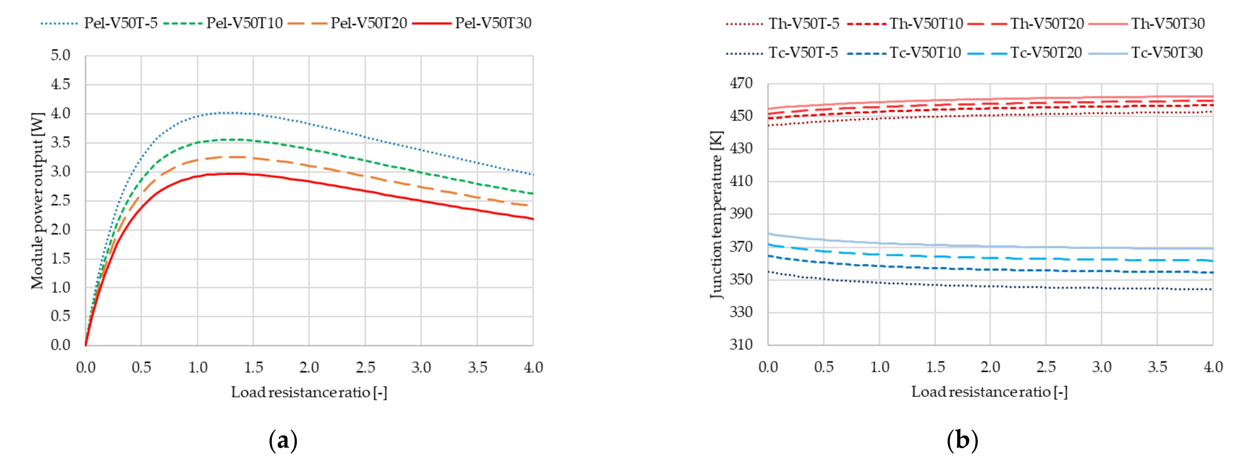
5. Results and Discussions

The model (Figure 13) was validated based on tests performed by Fagehi et al. [32]. In their work, Fagehi et al. [32] used a liquid (water) heat exchanger on the cold side which demanded a series of changes to the cold side heat exchanger model (not included in this study, but available upon request).

The comparison between the simulated and measured values is presented in Figure 14. Fagehi et al. [32] measured the junction temperatures, current, and voltage directly, while they calculated the power using two methods. The power designated with P_{el_Temp_I} is calculated using the junction temperatures, electric current, and the ideal thermoelectric equations; whereas, P_{el_V_I} was determined based on the measured voltage and current. Similar to the results of Fagehi et al. [32] the simulation results were closer to the power values determined using the junction temperatures, electric current, and the ideal thermoelectric equations. The average and matched load resistance errors for the junction temperatures, power output, current, voltage, and efficiency are listed in

Table 2. Comparison of calculated and measured values at peak measured power.

Parameter	Th [°C]	Tc [°C]	Pel [W]	I [A]	V [V]	ηth [-]
Average error [%]	0.15	0.33	12.73/1.77	6.82	0.52	0.93
Error at matched load resistance [%]	0.11	0.45	10.46/3.50	2.99	0.38	1.8

. The possible causes of differences are: Measurement accuracy, the use of ideal equations, effective material properties, as well as constant values for both the thermoelectric properties and gas properties. In addition, this effort neglects the Thomson coefficient, radiative heat transfer, and the thermal spread resistance. Another possible source of error is the extraction of data from the graphs presented in literature by using a digital tool. Despite all the uncertainties, there is a reasonable agreement between the calculated and the measured values.

As previously mentioned, Fagehi et al. [32] used a liquid (water) heat exchanger on the cold side. The same cold side temperature can be achieved by using air as the cooling fluid, but this poses an issue due to the very low thermal conductivity of air. This can be resolved by increasing the flow velocity and, to test this theory, the water cold side heat exchanger model (used only for the validation) was replaced with an air heat exchanger (similar to the one used on the hot side). Then, the air flow velocity on the cold side was adjusted to achieve a T_c value as close as possible to that obtained with the validated model (Figure 14). The required flow velocity was determined to be 13.1 m/s (or 47.2 km/h) and appears feasible for highway trucks and buses running at a constant speed. Here, the main advantages of utilizing air would be the lower weight and space requirements of the system, as well as a reduced complexity. Furthermore, a proper design of the flow passage to the cold side can allow for high air velocities; thus, leading to even greater temperature gradients than in the case of the liquid coolant solution. The main disadvantages of this solution are that the temperature gradient and, consequently, the power output depends on vehicle speed and outside temperature (still less than the coolant temperature). Also, this solution is not feasible for stationary engines.

To test the possible output of such a TEG, 16 test cases (

Table 3. Test cases for cold side heat exchanger using air as cooling fluid.

Case	Tair,-5 [°C]	Tair,10 [°C]	Tair,20 [°C]	Tair,30 [°C]
Vair,50 = 13.9 [m/s]	−5	10	20	30
Vair,80 = 22.2 [m/s]
Vair,90 = 25.0 [m/s]
Vair,120 = 33.3 [m/s]

) were evaluated with varying air temperatures (T_air) and air flow velocities (V_air). For the hot side, the temperature of the exhaust gases was set at 250 °C with a flow velocity of 19.1 m/s (12 L engine running at 1500 min⁻¹, with an exhaust pipe diameter of 100 mm). For brevity, only the results for 50 and 90 km/h are presented here with the others are available upon request. Regarding case notation, “V” stands for velocity and “T” for temperature. The values following “V” and “T” are the velocity (in km/h) and temperature (in °C) values for that case (e.g., V50T-5 = velocity of 50 km/h and temperature of −5 °C). For this study it was assumed that the hot and cold side fluid temperatures and flow velocities are uniform and constant, but also that there is a uniform temperature distribution on the TEG and TEM surface. Furthermore, the simulation was performed for only one TEM. Consequently, when considering the desired number of TEMs this will result in an overprediction of the power output.

Table 4. Results for cold side heat exchanger using air as cooling fluid.

Parameters	Case
	V50T-5	V50T10	V50T20	V50T30	V90T-5	V90T10	V90T20	V90T30
Pmax [W]	4.023	3.562	3.260	2.972	4.568	4.043	3.702	3.376
Th [K]	449.2	453.5	456.4	459.3	444.6	449.0	452.1	455.2
Tc [K]	347.6	357.6	364.7	371.7	336.3	347.1	354.6	362.0
ΔT [K]	101.7	95.9	91.8	87.6	108.3	101.9	97.5	93.1

and Figure 15 and Figure 16 show the results for the two different velocities 50 and 90 km/h. Analysis of the results finds that both the higher air flow velocity on the cold side and a lower ambient temperature increase the output of the TEG. Decreasing the air temperature raises the temperature gradient and the power output, but also reduces the temperature of the hot side junction to that below the maximum allowable value of the TEM. This is because the hot side heat flow rate is constant. To further augment the output of the TEG, it would be necessary to increase the heat flow rate on the hot side (either by increasing the exhaust temperature or the flow velocity). Consequently, a high TEG output requires not only a good HX, but also a suitable heat extraction strategy.

6. Conclusions

Considering the vast amounts of wasted thermal energy from internal combustion engines, the study of thermoelectric power generation is necessary as a possibility to increase overall energy efficiency. Thermoelectric devices are environmentally friendly and have numerous other advantages including the lack of moving parts, high reliability, the direct conversion of thermal energy into electrical energy, as well as low maintenance requirements. However, the main disadvantage of such devices is their low efficiency owing to the small $\mathrm{Z}\overline{\mathrm{T}}$ values currently found in commercial devices.

In the present study, two Simulink models are presented (see Appendix A for detailed Simulink blocks). The first model was created based on the work of Lee et al. [20] to estimate thermoelectric parameters of a thermoelectric module. The validation showed that, even though the temperature dependency of the thermoelectric parameters was neglected, there is a relatively good agreement with experimental data.

Furthermore, a TEG model was proposed and validated for power output estimations in the case of exhaust gas thermoelectric generators. Model validation was accomplished using the results of Fagehi et al. [32]. For the validation, the cold side heat exchanger model was adapted to match the cooling method of the authors with reasonable agreement. The next step was to study the possibility of using air as the cooling fluid and to achieve the same cold side temperature, the flow velocity of the cold air was adjusted (an air velocity of 13.1 m/s showed a relatively good agreement).

After determining that similar results can be obtained with air as the cooling fluid, a parametric study was performed to show the potential of such a system for ICE exhaust coupling. The test conditions (used as input data for the cold side heat exchanger) considered a vehicle (with a respectively large engine capacity) traveling at different speeds (50, 80, 90, and 120 km/h) under dissimilar ambient air temperatures (−5, 10, 20, and 30 °C). The results showed that either a high air velocity or a low outside temperature leads to greater TEG power output. For the analyzed cases, the peak power output was 4.568 W for a temperature gradient of 108.3 K. It was also found that increasing the heat rejection on the cold side requires a simultaneous growth in heat input at the hot side to facilitate a favorable temperature gradient and, therefore, the power output of the TEG. Overall, this demonstrates that it is feasible to install an air-cooled TEG on a heavy-duty vehicle running at constant speed.

References

1. Hariram, A.; Koch, T.; Mårdberg, B.; Kyncl, J. A Study in Options to Improve Aerodynamic Profile of Heavy-Duty Vehicles in Europe. Sustainability 2019, 11, 5519. [Google Scholar] [CrossRef] [Green Version]
2. Márquez-García, L.; Beltrán-Pitarch, B.; Powell, D.; Min, G.; García-Cañadas, J. Large Power Factor Improvement in a Novel Solid–Liquid Thermoelectric Hybrid Device. ACS Appl. Energy Mater. 2018, 1, 254–259. [Google Scholar] [CrossRef]
3. Thacher, E.F.; Helenbrook, B.T.; Karri, M.A.; Richter, C.J. Testing of an automobile exhaust thermoelectric generator in a light truck. Proc. Inst. Mech. Eng. Part D J. Automob. Eng. 2007, 221, 95–107. [Google Scholar] [CrossRef]
4. Liu, X.; Deng, Y.D.; Li, Z.; Su, C.Q. Performance analysis of a waste heat recovery thermoelectric generation system for automotive application. Energy Convers. Manag. 2015, 90, 121–127. [Google Scholar] [CrossRef]
5. Yu, C.; Chau, K.T. Thermoelectric automotive waste heat energy recovery using maximum power point tracking. Energy Convers. Manag. 2009, 50, 1506–1512. [Google Scholar] [CrossRef]
6. Karri, M.A.; Thacher, E.F.; Helenbrook, B.T. Exhaust energy conversion by thermoelectric generator: Two case studies. Energy Convers. Manag. 2011, 52, 1596–1611. [Google Scholar] [CrossRef]
7. Yu, S.; Du, Q.; Diao, H.; Shu, G.; Jiao, K. Effect of vehicle driving conditions on the performance of thermoelectric generator. Energy Convers. Manag. 2015, 96, 363–376. [Google Scholar] [CrossRef]
8. Ma, X.; Shu, G.; Tian, H.; Yang, H.; Chen, T. Optimization of length ratio in segmented thermoelectric generators for engine’s waste heat recovery. Energy Procedia 2019, 158, 583–588. [Google Scholar] [CrossRef]
9. Deng, Y.D.; Liu, X.; Chen, S.; Tong, N.Q. Thermal Optimization of the Heat Exchanger in an Automotive Exhaust-Based Thermoelectric Generator. J. Electron. Mater. 2013, 42, 1634–1640. [Google Scholar] [CrossRef]
10. Marvão, A.; Coelho, P.J.; Rodrigues, H.C. Optimization of a thermoelectric generator for heavy-duty vehicles. Energy Convers. Manag. 2019, 179, 178–191. [Google Scholar] [CrossRef]
11. He, W.; Wang, S.; Zhao, Y.; Li, Y. Effects of heat transfer characteristics between fluid channels and thermoelectric modules on optimal thermoelectric performance. Energy Convers. Manag. 2016, 113, 201–208. [Google Scholar] [CrossRef]
12. Fan, L.; Zhang, G.; Wang, R.; Jiao, K. A comprehensive and time-efficient model for determination of thermoelectric generator length and cross-section area. Energy Convers. Manag. 2016, 122, 85–94. [Google Scholar] [CrossRef]
13. Yu, S.; Du, Q.; Diao, H.; Shu, G.; Jiao, K. Start-up modes of thermoelectric generator based on vehicle exhaust waste heat recovery. Appl. Energy 2015, 138, 276–290. [Google Scholar] [CrossRef]
14. Wang, Y.; Li, S.; Zhang, Y.; Yang, X.; Deng, Y.; Su, C. The influence of inner topology of exhaust heat exchanger and thermoelectric module distribution on the performance of automotive thermoelectric generator. Energy Convers. Manag. 2016, 126, 266–277. [Google Scholar] [CrossRef]
15. Du, Q.; Diao, H.; Niu, Z.; Zhang, G.; Shu, G.; Jiao, K. Effect of cooling design on the characteristics and performance of thermoelectric generator used for internal combustion engine. Energy Convers. Manag. 2015, 101, 9–18. [Google Scholar] [CrossRef]
16. Goldsmid, H.J. Introduction to Thermoelectricity, 2nd ed.; Springer: Berlin/Heidelberg, Germany, 2016; ISBN 978-3-662-49255-0. [Google Scholar]
17. Rowe, D.M. Thermoelectrics Handbook—Macro to Nano; CRC/Taylor & Francis: Boca Raton, FL, USA, 2006. [Google Scholar]
18. Kumar, P.M.; Jagadeesh-Babu, V.; Subramanian, A.; Bandla, A.; Thakor, N.; Ramakrishna, S.; Wei, H. The Design of a Thermoelectric Generator and Its Medical Applications. Designs 2019, 3, 22. [Google Scholar] [CrossRef] [Green Version]
19. Wang, H.; McCarty, R.; Salvador, J.R.; Yamamoto, A.; König, J. Determination of Thermoelectric Module Efficiency: A Survey. J. Electron. Mater. 2014, 43, 2274–2286. [Google Scholar] [CrossRef]
20. Lee, H.; Attar, A.M.; Weera, S.L. Performance Prediction of Commercial Thermoelectric Cooler Modules using the Effective Material Properties. J. Electron. Mater. 2015, 44, 2157–2165. [Google Scholar] [CrossRef]
21. Zhang, H.Y. A general approach in evaluating and optimizing thermoelectric coolers. Int. J. Refrig. 2010, 33, 1187–1196. [Google Scholar] [CrossRef]
22. KRYOTHERM. TGM-199-1.4-0.8. Available online: https://kryothermtec.com/assets/dir2attz/ru/TGM-199-1.4-0.8.pdf (accessed on 4 January 2021).
23. KRYOTHERM. TGM-127-1.4-2.5. Available online: http://kryothermtec.com/assets/dir2attz/ru/TGM-127-1.4-2.5.pdf (accessed on 4 January 2021).
24. Teertstra, P.; Yovanovich, M.M.; Culham, J.R.; Lemczyk, T. Analytical forced convection modeling of plate fin heat sinks. In Proceedings of the Fifteenth Annual IEEE Semiconductor Thermal Measurement and Management Symposium (Cat. No.99CH36306), San Diego, CA, USA, 9–11 March 1999; pp. 34–41. [Google Scholar]
25. Lee, H. Thermoelectrics: Design and Materials; John Wiley & Sons: Hoboken, NJ, USA, 2016. [Google Scholar]
26. Gnielinski, V. New equations for heat and mass transfer in turbulent pipe and channel flow. Int. Chem. Eng. 1976, 16, 359–368. [Google Scholar]
27. Petukhov, B.S. Heat Transfer and Friction in Turbulent Pipe Flow with Variable Physical Properties. In Advances in Heat Transfer; Hartnett, J.P., Irvine, T.F., Greene, G.A., Cho, Y.I., Eds.; Elsevier: Amsterdam, The Netherlands, 1970; Volume 6, pp. 503–564. ISBN 0065-2717. [Google Scholar]
28. Cengel, Y.; Ghajar, A. Heat and Mass Transfer: Fundamentals and Applications, 6th ed.; McGraw-Hill Education: New York, NY, USA, 2020; ISBN 978-981-315-896-2. [Google Scholar]
29. Kumar, S.; Heister, S.D.; Xu, X.; Salvador, J.R.; Meisner, G.P. Thermoelectric Generators for Automotive Waste Heat Recovery Systems Part II: Parametric Evaluation and Topological Studies. J. Electron. Mater. 2013, 42, 944–955. [Google Scholar] [CrossRef]
30. Cengel, Y.; Cimbala, J. Fluid Mechanics Fundamentals and Applications, 4th ed.; McGraw-Hill Education: New York, NY, USA, 2017; ISBN 978-1259696534. [Google Scholar]
31. Bergman, T.; Adrienne, L.; Frank, I.; David, D. Fundamentals of Heat and Mass Transfer; John Wiley & Sons, Inc.: New York, NY, USA, 2011; ISBN 978-0470-50197-9. [Google Scholar]
32. Fagehi, H.; Attar, A.; Lee, H. Optimal Design of an Automotive Exhaust Thermoelectric Generator. J. Electron. Mater. 2018, 47, 3983–3995. [Google Scholar] [CrossRef]
Figure 1. Thermoelectric couple operating as a generator.
Applsci 11 01340 g001
Figure 2. Thermoelectric module operating as a generator (based on [18]).
Applsci 11 01340 g002
Figure 3. Simulink model for determining effective properties (values for TGM-127-1.4-2.5).
Applsci 11 01340 g003
Figure 4. Manufacturer data compared to calculated data at matched load resistance conditions for TGM-199-1.4-0.8: (a) Module power; (b) module current; (c) module voltage; (d) module power and voltage with respect to current; and (e) module efficiency.
Applsci 11 01340 g004
Figure 5. Manufacturer data compared to calculated data at matched load resistance conditions for TGM-127-1.4-2.5: (a) Module power; (b) module current; (c) module voltage; (d) module power and voltage with respect to current; and (e) module efficiency.
Applsci 11 01340 g005
Figure 6. Hot side heat exchanger.
Applsci 11 01340 g006
Figure 7. Side view of module section.
Applsci 11 01340 g007
Figure 8. Integration of thermoelectric module in a thermoelectric generator.
Applsci 11 01340 g008
Figure 9. (a) Thermoelectric generator (TEG) temperatures of interest; (b) thermal resistance network for a CV; (c) simplified thermal resistance network for calculating Tc; and (d) simplified thermal resistance network for calculating Th.
Applsci 11 01340 g009
Figure 10. Integration of thermoelectric module in a thermoelectric generator.
Applsci 11 01340 g010
Figure 11. Areas used for calculating the pressure loss due to flow contraction and expansion.
Applsci 11 01340 g011
Figure 12. Solution methodology flow chart.
Applsci 11 01340 g012
Figure 13. Simulink model with two heat exchangers (red—hot side and blue—cold side), aluminum blocks for thermal spread (light grey), the TEM between, and the thermal resistance network on right side.
Applsci 11 01340 g013
Figure 14. TEG model validation highlighting the difference between the simulated and measured values of (a) the electrical power output, (b) hot and cold junction temperatures, (c) current, and (d) voltage for two different types of cold side heat exchangers: Water (W_sim) and air (air_sim).
Applsci 11 01340 g014
Figure 15. (a) Module power output, (b) junction temperature, (c) module current, and (d) module voltage with respect to the load resistance ratio for a velocity of 50 km/h at various temperatures (−5, 10, 20, and 30 °C).
Applsci 11 01340 g015aApplsci 11 01340 g015b
Figure 16. (a) Module power output, (b) junction temperature, (c) module current, and (d) module voltage with respect to the load resistance ratio for a velocity of 90 km/h at various temperatures (−5, 10, 20, and 30 °C).
Applsci 11 01340 g016