1. Introduction
Currently, the use of paper money remains one of the main options for the exchange of products and services. However, one of the remaining problems is the detection of counterfeit banknotes, which increasingly resemble originals, making it difficult for someone who is not an expert in the field to detect them. On the other hand, there are machines for detecting counterfeit banknotes [
1]; however, these are often expensive, so the identification and retention of counterfeits ends up falling on financial and government entities, with minimal community involvement [
2].
In order to solve this problem and to present alternative solutions, in the state-of-the-art, there are proposals based on classical computer vision techniques. For example, from histogram equalization [
3], nearest neighbor interpolation [
4], genetic algorithms [
5] and fuzzy systems [
6]. However, the main problem of this type of methods is its low capacity of generalization for new examples as well as its low accuracy. Another group corresponds to those methods based on deep learning (DL) using convolutional neural networks (CNNs) [
7,
8,
9], which have outperformed to the classic machine learning techniques [
10] and humans too [
11] in classification tasks.
Considering the current importance of the CNNs in the field of computer vision, there are some proposals in the area of banknote recognition and counterfeit detection. For example, transfer learning (TL) with Histograms of Oriented Gradients for Euro banknotes [
12], a YOLO net for Mexican banknotes [
13] or custom CNN architectures for dollar, Jordanian dinar and Won Koreano banknotes [
14,
15] have been proposed. However, one of the main disadvantages of proposals using CNNs that focus on fake banknote recognition is that there is no clarity about which design strategy is more appropriate, either custom or by transfer learning. When using transfer learning-based networks, there are many types of patterns that the network has learned, but they are not specific to the current task. On the other hand, custom networks are trained with a much smaller dataset than the pre-trained networks, but they specifically learn the patterns of this type of classification task. Another shortcoming found in the literature is that the impact of the freezing point (FP) of the pre-trained network on the performance of the classifier has not been analysed.
According to the above, the main contributions of this research are as follows:
A methodology to identify the best freezing point in models by transfer learning, for three different types of architectures: sequential, residual and Inception is proposed.
A custom model inspired in AlexNet that has faster inference times in an embedded system than models by transfer learning is proposed.
A comparative study for the fake banknote recognition task between a custom model and several models obtained by transfer learning, in terms of accuracy and inference times is given.
The rest of the paper is organized as follows.
Section 2 presents the background of Convolutional Neural Networks and transfer learning.
Section 3 shows the proposed system of image acquisition and the used dataset.
Section 4 explains the proposed methodology for selecting the freezing point in the design by transfer learning.
Section 5 presents the proposed custom model.
Section 6 shows the results of the research. Finally,
Section 7 summarizes the work.
2. Background
This section explains the main concepts involved in this work. First, the general concepts of CNNs are addressed followed by TL, and finally, the main CNN architectures that have been used in the literature are presented.
2.1. Convolutional Neural Networks
CNNs are one of the most widespread DL techniques, especially in computer vision, since they focus mainly on the extraction and learning of features in images [
16]. In general, CNNs are based on the application of a kernel to the data (i.e., sum of the products generated between the elements of the kernel and those of the matrix) [
17]. In Equation (
1), the traditional convolution operation is presented; however, in the CNN, the function is not inverted, so in fact a cross-correlation operation is performed (see Equation (
2)).
where I represents the input image, K the applied kernel, i and j are the initial position of the image from which the filter will start operating, and m and n are the position of the filter element.
In addition to convolution, specific layers are used in CNNs to improve performance. The following is a brief explanation of these.
Rectified Linear Unit (ReLU): The ReLU is an activation function that is applied to the feature map, resulting from the convolution of the filters with the input array. It helps to prevent the vanishing gradient problem, while maintaining the positive features [
18].
Pooling: This type of layer is applied to reduce the size of the feature maps to decrease computing costs. To achieve this objective, similar semantic features are grouped into one, thus obtaining a reduced feature map that keeps the main characteristics of the original input [
19].
Fully Connected (FC): These layers allow for a more extensive learning of the features. They can be represented as a traditional neural network, or also as
convolutions [
17].
2.2. CNN-Architectures
In the state-of-the-art, different types of CNNs architectures have been proposed. The use of one or another may depend on the type of application; for example, to have greater complexity, or a variety of features, to reduce inference times, and even to avoid the vanishing gradient problem. Below are some of the main architectures that have been used in the literature.
2.2.1. Sequential
This is the deep learning architecture pioneered in the literature [
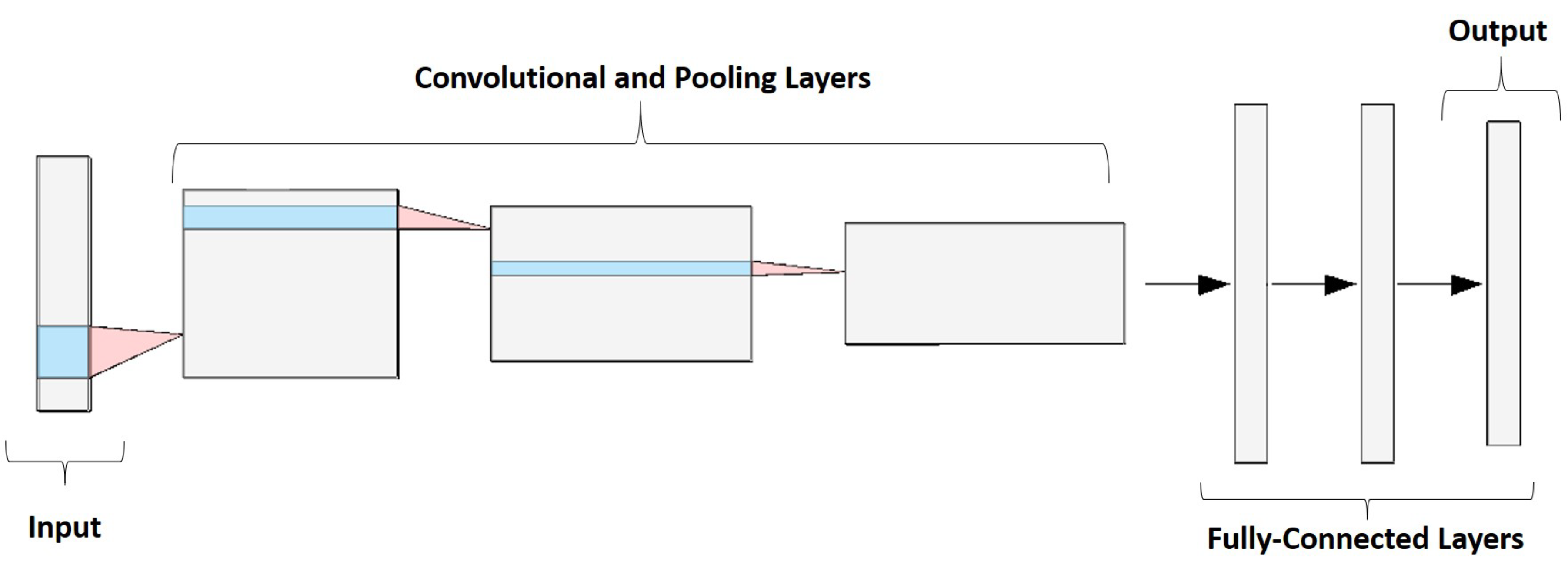
20]. It consists of sequential layers of convolution and pooling type, whose task is to extract patterns from the image. Typically, as the network gets deeper, the number of filters in convolutional layers increases and the number of rows (H) and columns (W) decreases. Finally, fully connected layers are added, which perform the classification (see
Figure 1). The main advantage of this type of architecture is the ease of implementation, while its disadvantage is that it requires great depth if you want to learn more complex patterns, generating a vanishing gradient problem.
2.2.2. Residual
CNNs at greater depth, i.e., with a greater number of convolution layers, can extract more features that facilitate learning of the network. However, with increasing depth, the vanishing gradient problem is presented. The residual CNNs arise to give a solution to this problem [
11], by means of adding to the output of a convolutional layer the input of a previous layer (see
Figure 2).
2.2.3. Inception
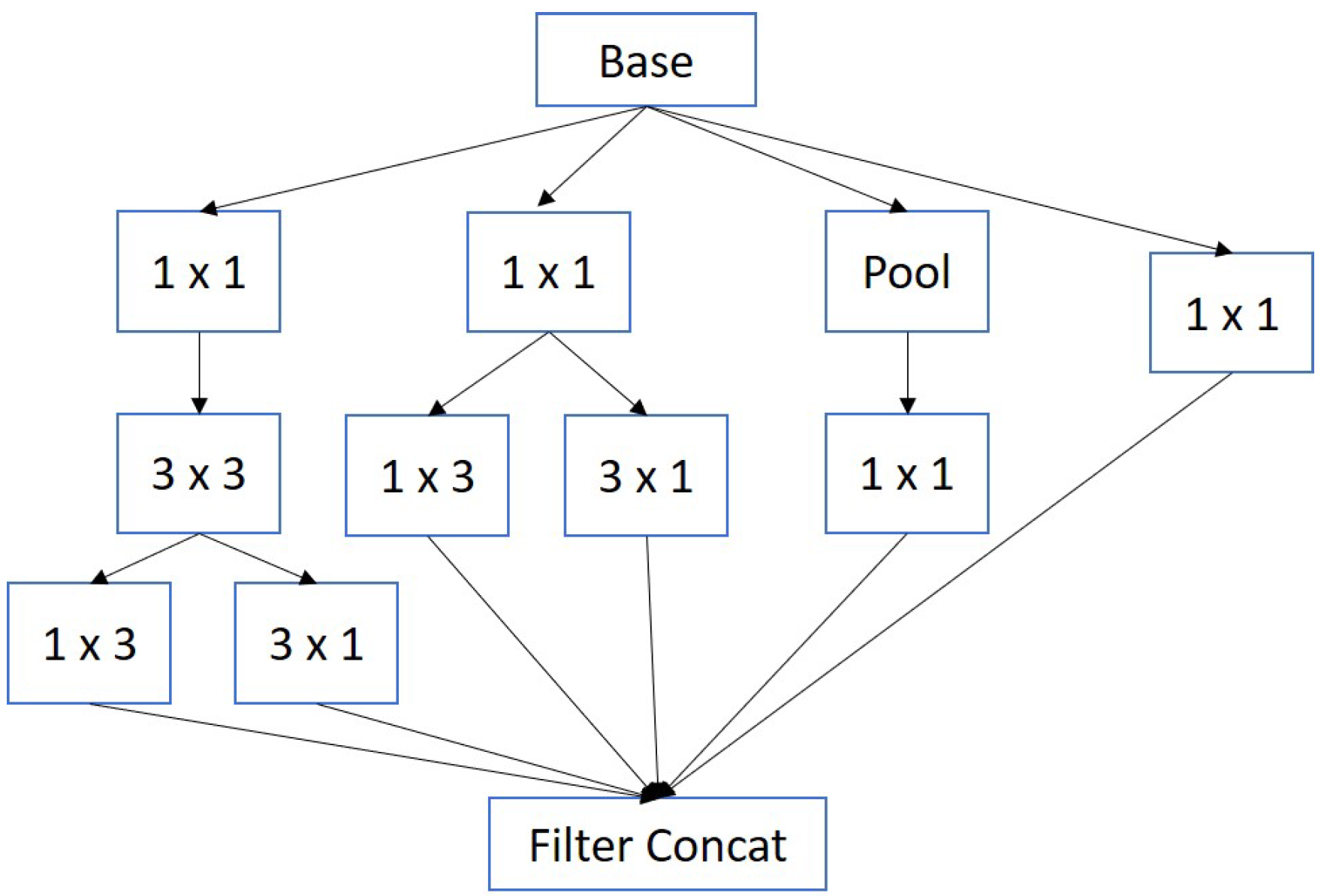
When designing CNN architectures, there are no specific rules about what size the filters should be or whether a pooling layer should be applied. In
Figure 3, a block of an Inception-type architecture is presented, where different sizes of filters, and even pooling layers, can be applied at each stage of the network [
22].
2.3. Transfer Learning (TL)
When training a neural network, it is useful to have a dataset of thousands of images that allows the network to learn different patterns to improve the classification task. However, in many cases, it is not easy to have a large dataset for the specific task. Therefore, TL arises as a solution to this problem, since networks that have already been pre-trained with thousands or millions of images (e.g., ImageNet [
23], COCO [
24]) are available [
25]. This is possible because of the large number of patterns previously learned by pre-trained models from large sets of images can be useful in a new classification task.
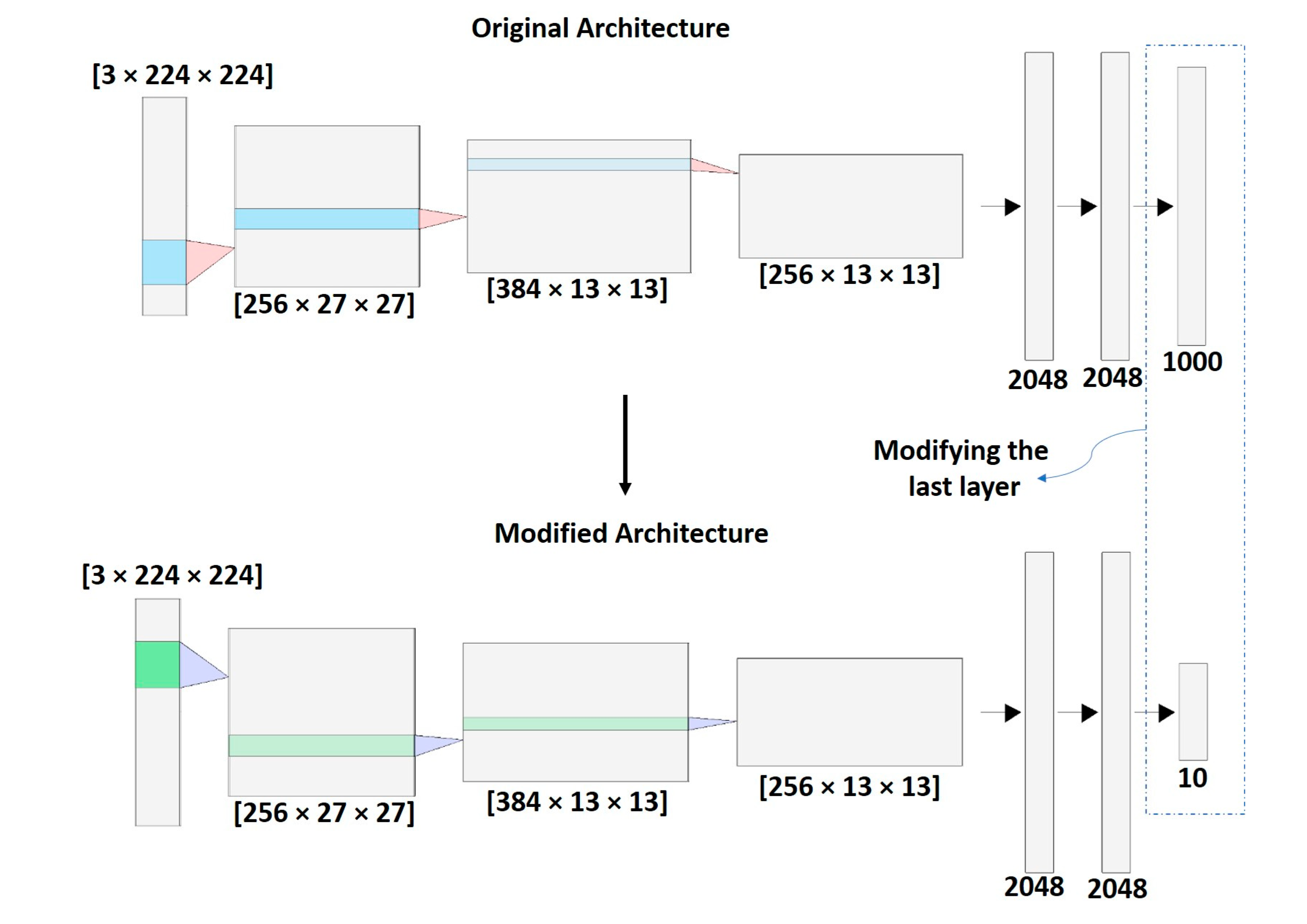
Figure 4 shows an example of TL in a CNN, which replaces the last layer of the original architecture that initially classified 1000 object types, so that now it classifies 10 object types. The rest of the parameters learned from the pre-trained network are transferred to the new network.
3. Data Acquisition System
This section presents the proposed system for capturing and identifying banknote images. Additionally, the characteristics of the dataset and how it was used for training, validation and testing are given.
3.1. Prototype Design
Each family of banknotes has different security features that allow to identify its authenticity. Generally, Colombian banknotes stand out for having holograms, magnetic strips, and security features that are only visible when exposed to ultraviolet light (UV). Taking into account the existing problems due to the cost of magnetic band sensors and the ease of making counterfeits in visible light [
26], we have chosen to design a system that highlights the characteristics of UV light.
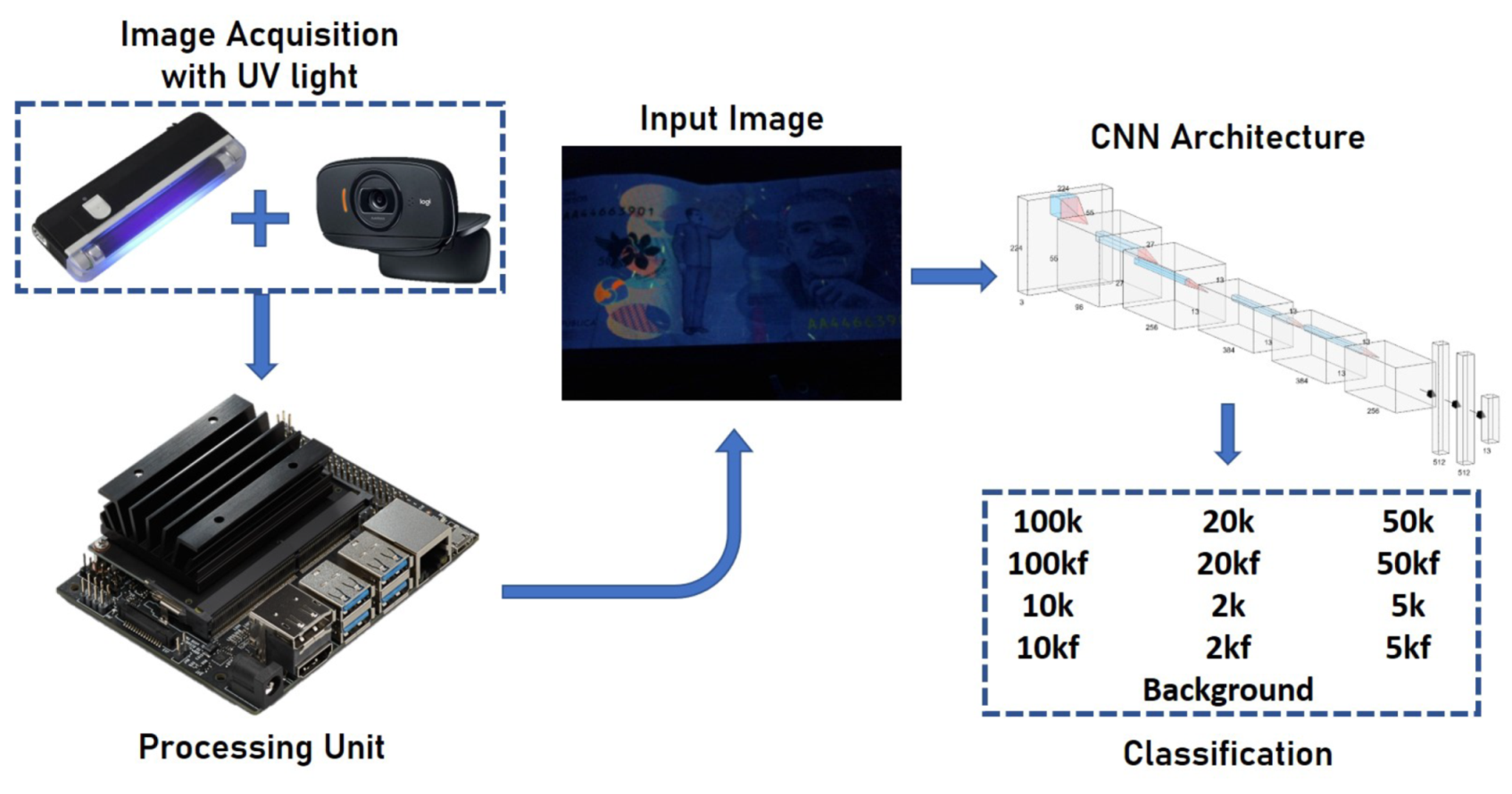
Figure 5 shows the proposed scheme. The banknotes should be placed in a dark compartment (little natural light). A UV light lamp with an average wavelength of 365 nm is activated on the banknotes, allowing the main security elements to be highlighted. These elements are captured by means of a web-cam (in this case, a Logitech c525) and transferred to an embedded system (Jetson Nano). This image is the CNN entry that returns the name of the class in which it was classified.
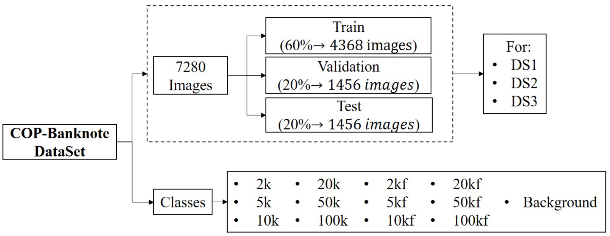
Six types of banknotes and their corresponding counterfeit were taken into account: 2k, 2kf, 5k, 5kf, 10k, 10kf, 20k, 20kf, 50k, 50kf, 100k, 100kf, where f corresponds to a fake banknote and k corresponds to thousands of Colombian peso, COP (e.g., 10k is 10,000 COP, which is approximately 3 USD.). An additional class is added to the background so that if there is no banknote in the captured image, the network will not classify it in any of the other classes.
3.2. DataSet
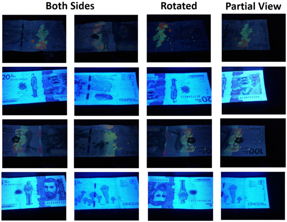
Using the proposed system, 7280 images were captured and stored (560 images per class), including rotations, partial views of the banknotes and non-aligned banknotes (see
Figure 6). However, given the environmental conditions, natural light may leak into the system. To solve this problem, data augmentation by varying lighting conditions was performed [
27], to the training data set during the training stage of the network.
A summary of the distribution of the dataset is presented in
Figure 7. Without considering the data augmentation, the dataset has a total of 7280 images, where the distribution in the classes is balanced. The dataset is divided into three folders, as follows: 60% is for training, 20% for validation and 20% for testing, as suggested in [
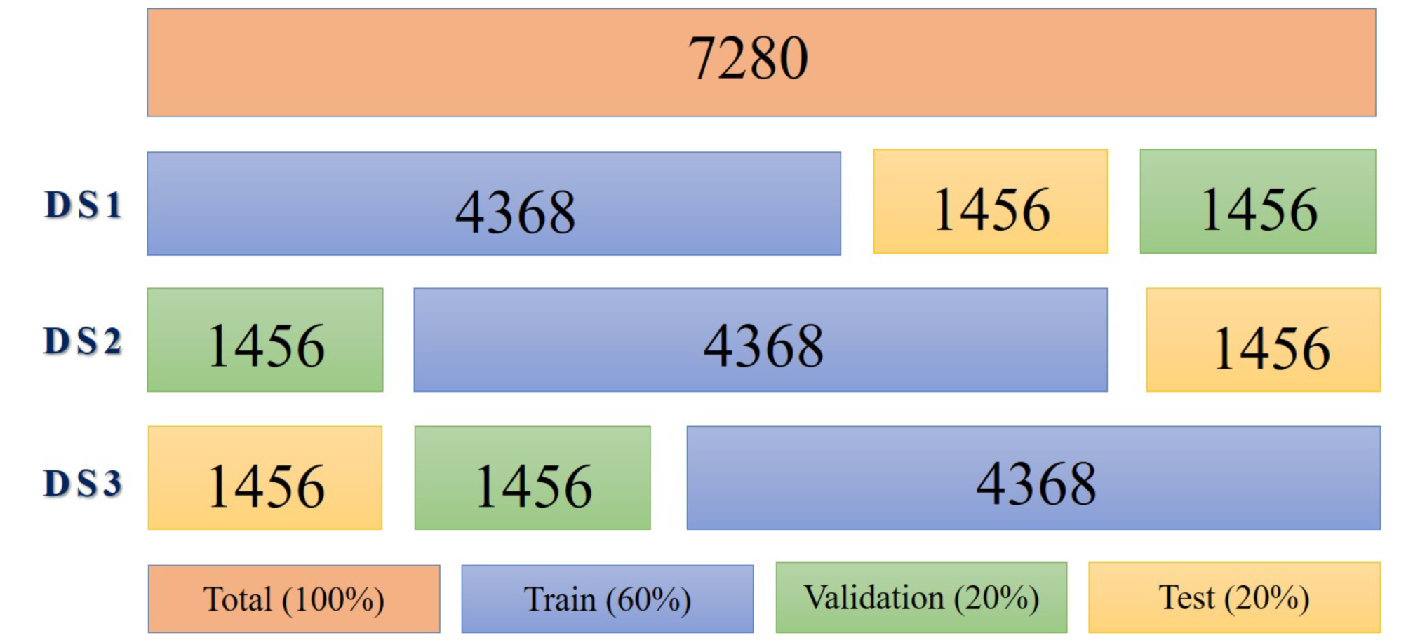
29]. In addition, the elements in the dataset are organized in three different ways—DS1, DS2 and DS3—to apply triple cross-validation [
30,
31].
Each DS contains all the images and the same percentages of distribution, the only difference being the specific images that belong to the training, validation or test folders (See
Figure 8). With the results of DS1, DS2 and DS3, we calculate the average accuracy.
4. Transfer-Learning-Based Models and Freezing Points (FP)
This section presents the proposed methodology for training the models by TL. First, the architectures to be evaluated are selected. Then, the ways to perform TL with FP are established. Finally, the algorithm developed to obtain each of the models trained by TL is presented.
As a starting point in models based on transfer learning, it is necessary to take into account that there are three main types of architectures in deep learning for computer vision: sequential, residual and inception. In each category, there are important neural network architectures that have been the base model for further development. In our current research, AlexNet and SqueezeNet were selected in the category of sequential architectures, the first because it pioneered parallel training on GPUs and overcame classical machine learning techniques in image pattern recognition [
10], the second because it proposed a type of layer called fire, reducing the number of parameters in AlexNet [
32]. In the category of residual networks, ResNet18 [
11] was selected because it has been used in many transfer learning works with high-performance results. Finally, InceptionV3 [
33] was selected in the inception category.
In addition to the selection of the pre-trained network, the freezing point of the network should be included, since in not all cases the same freezing point provides the necessary patterns for the classifier to make the decision. Thus, in this work, three FPs were analysed, as shown in
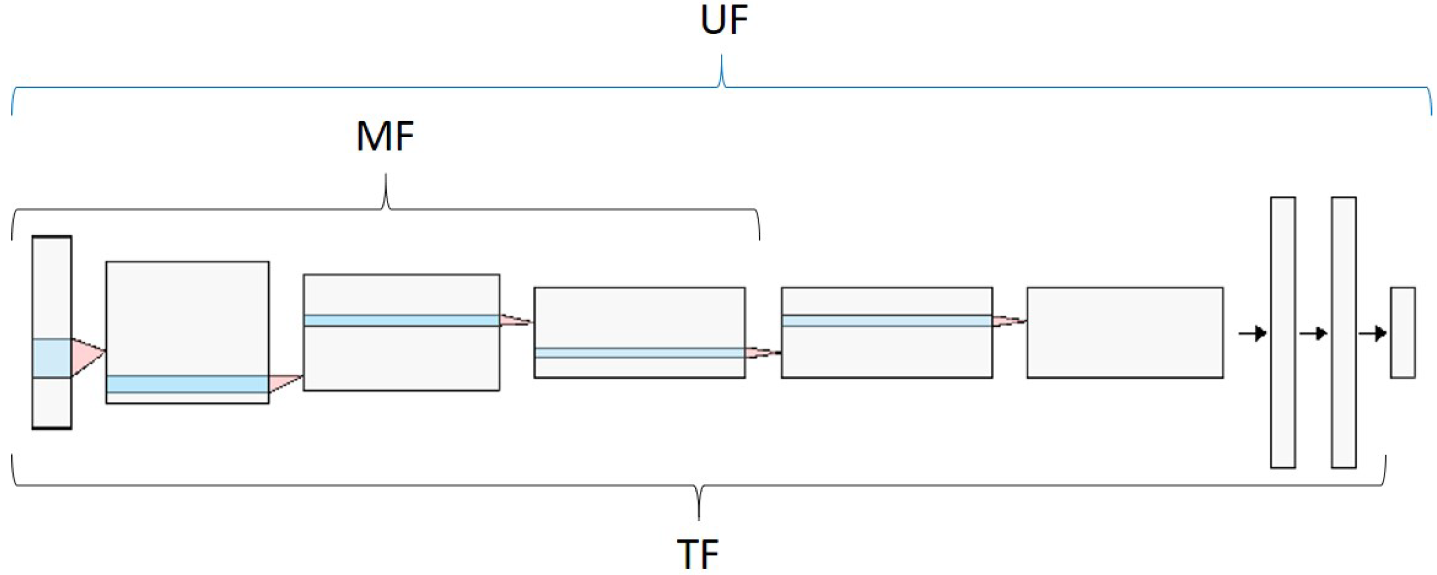
Figure 9: UF means that the whole network will be retrained, MF corresponds to the freezing of the parameters of the first half of the network, while in TF, all the parameters are frozen, except those of the last FC layer.
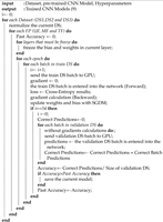
Considering that the dataset was organized in three different ways (i.e., DS1, DS2 and DS3), and that three FPs (i.e., UF, MF and TF) and four pre-trained architectures (i.e., AlexNet, SqueezeNet, ResNet18 and InceptionV3) were selected, 36 TL-based models are obtained. To train these models, the Algorithm 1 was applied, whose inputs are the dataset, the pre-trained model and the hyperparameters, and whose output are the trained models. First, one of the datasets (DS) is selected and normalized. Then, one of the FP is established in the network. In the third stage, the training begins, in which the current batch is sent to the GPU to make all the calculations. Once the batch is in the GPU, the gradient is established in 0 and the batch is entered into the network making the forward. The network returns the losses which are used in the backward, and afterward, the network weights are updated. Every 54 iterations, which is approximately 10 times per epoch, the network performance is verified with the validation dataset of the current DS. If the performance is higher in terms of accuracy, the model is saved. Finally, once the network training is finished, the loops that allow for changes to be made to the DS and the FP are repeated.
| Algorithm 1: CNN-TL-Train algorithm. |
![Applsci 11 01281 i001 Applsci 11 01281 i001]() |
5. Custom Model
This section presents the proposed architecture based on CNN for the detection of counterfeits and banknote denominations. Additionally, an analysis of the features learned by the proposed model is carried out.
5.1. Architecture
The behavior of the supervised deep learning models depends largely of the dataset used for their training. For this reason, in the CNNs, there are no specific rules about the number of convolutional layers, number of filters per layer, or quantity of fully connected layers that it should have. Considering that one of the purposes of this research is to identify whether it is more appropriate to use TL-based models or a model trained from scratch, in the task of detecting denominations and counterfeit banknotes, an AlexNet-inspired model is proposed, but with the following differences: the number of filters in the convolutional layers and the number of units in the fully connected layers (FC) (see
Figure 10). Therefore, the proposed custom network extracts fewer feature maps than those of AlexNet, and the classifier is more compact. In this network, the input image is
, followed by five convolutional layers and three FC layers. The aim is to obtain low, medium and high features, i.e., edges, textures, colour and shapes. The last FC layer has 13 outputs because there are 13 different classes. The activation function of the last layer is softmax to obtain the probability of belonging to each class [
34].
Table 1 shows the hyperparameters of the network. Only convolutional layers have trainable parameters. When stride (S) is higher than 1, the output shape is significantly lower than the input shape (i.e., the output shape of the previous layer). For example, for the first convolutional layer, the input shape was
and the output shape was
, because
. As the network becomes deeper, the size of the feature maps became smaller (i.e., the first (H) and second dimension (W) were reduced), but with more channels (i.e., the third dimension increases). For all convolutional layers, the ReLU activation function was used. Finally, two dropout layers were added to avoid overfitting.
Regarding the drawbacks when training models from scratch, the training time and the difficulty of the CNN to converge on suitable parameter values should be considered. To overcome this problem, the Xavier Method is used for the initialization of parameters, which is based on a uniform distribution according to Equation (
3), where
is the fan-in, and
is the fan-out from that layer [
35]. This method maintains equal variation across all layers of the network and avoids the saturation that occurs when initial parameters are mistakenly selected at random.
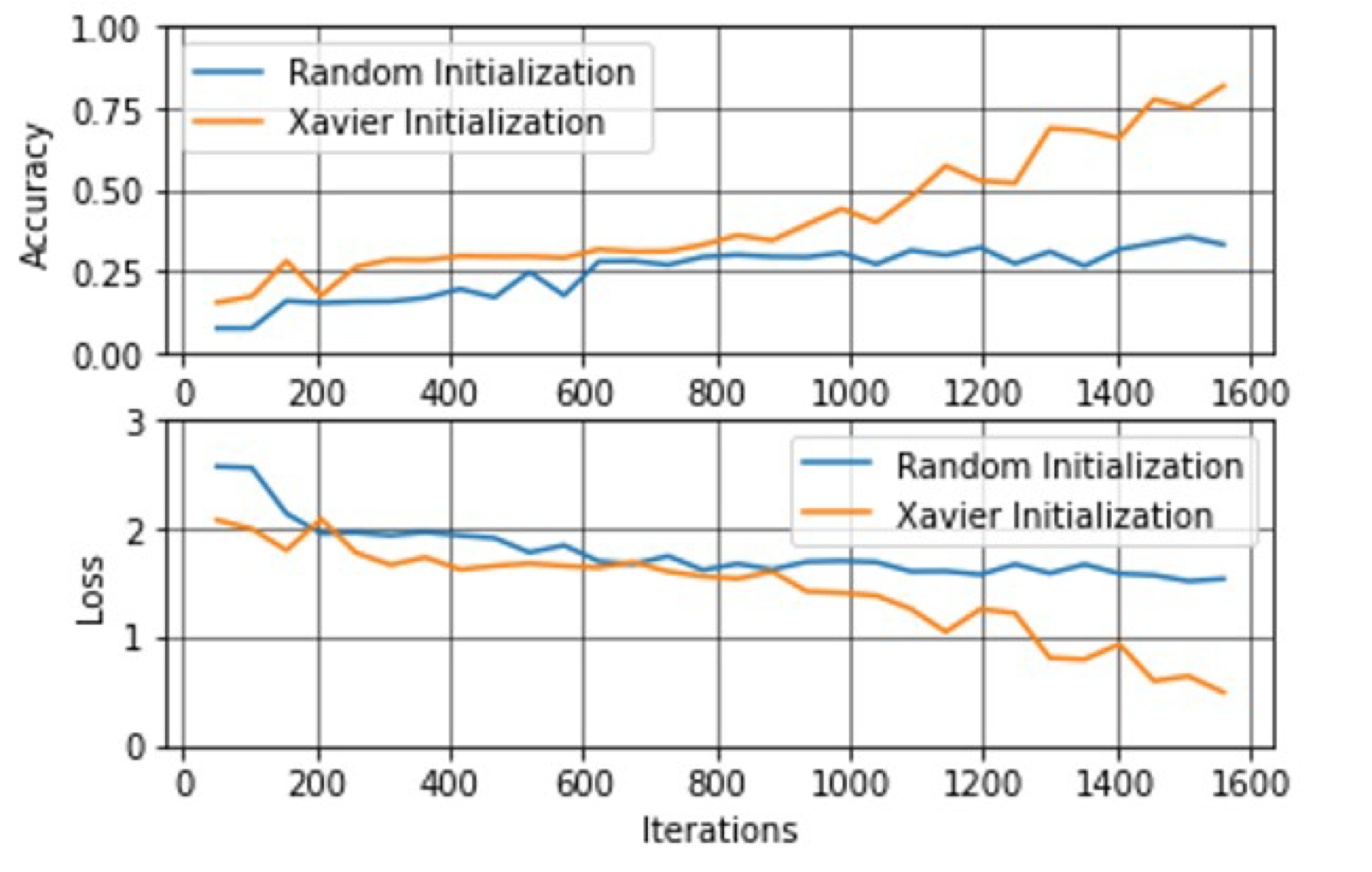
Figure 11 shows a comparison between a random initialisation and the Xavier method with the proposed dataset. It should be noted that as the iterations go by, the behaviour of the random initialization tends to remain constant while that of the Xavier method continues to improve the accuracy and decrease the error.
5.2. Feature Maps
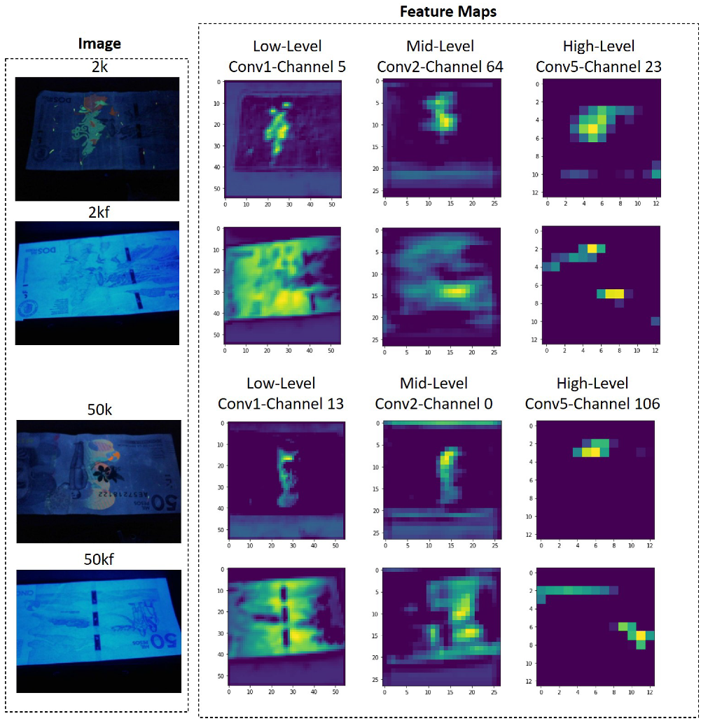
Figure 12 shows some feature maps of the custom model at different depth levels. Two examples of original and their counterfeit banknotes are presented (i.e., 2k with 2kf, and 5k with 5kf), with a clear differences in their feature maps. For counterfeit banknotes, a large part of the feature maps are activated, while in the case of original banknotes, only a small part related to the UV security mask is activated. This shows that the custom model trained with the proposed data set is able to learn the weights of its filters in order to identify original and counterfeit banknotes.
Additionally, the filters are able to learn to differentiate the denominations of the banknotes.
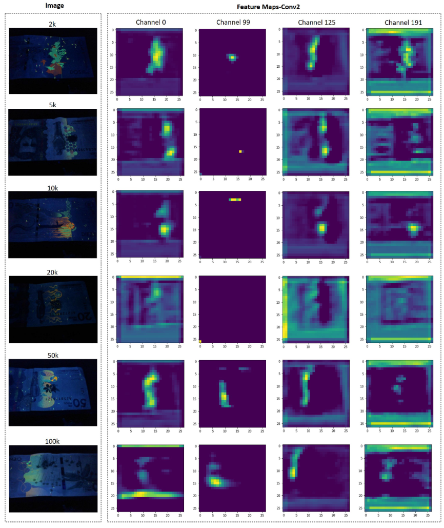
Figure 13 shows an example for the different denominations in the dataset, only for original banknotes. It should be noted that the feature maps of the 20k banknote on channel0 and channel125 are different in relation to other banknotes, just as the feature maps of the 50k and 100k banknotes of the channel99 differ from the other denominations. In the case of channel191, the feature map is activated not only in the UV mark, but in the background.
This shows that the network is capable of extracting patterns that allow it not only to identify whether a banknote is original or counterfeit, but also its denomination. Training the network with the dataset allows the model to adjust the weights of its filters (parameters) for the specific classification task. So, if you want to use the proposed network in another task, you will have to retrain the architecture with the corresponding dataset.
6. Results
To present and compare the results of the proposed models, this section is divided into six parts. The first part presents the conditions under which the experiments were developed, so that the results can be replicated by other researchers. The second and third parts show the results of TL-based and custom models, respectively. Next, the models are compared in terms of accuracy and inference times. The fifth part presents some recommendations to select the most appropriate model. Finally, the custom model is compared to some state-of-the-art works.
6.1. Experimental Settings
To ensure the replicability of the results given in this section, the training hyperparameters (see
Table 2) and the specifications of the hardware with which the tests were carried out are provided (see
Table 3). As shown in
Table 2, TL-based models and the custom model have the same training hyperparameters, except the one corresponding to the number of epochs, which for the custom model was 10. In the adjustment of the training hyperparameters, the random search methodology with close values was used, which has been widely used in other studies [
36,
37]. On the other hand,
Table 3 shows the hardware of the computer equipment on which all models were trained, as well as the characteristics of the embedded system that was used to calculate the CPU and GPU inference times of the trained models.
The accuracy values reported in
Section 6.2.2,
Section 6.2.3 and
Section 6.4 were calculated by applying the Equation (
4), which allows the average accuracy (
) to be obtained.
where
is True positive,
is True negative,
is False positive and
is False negative.
corresponds to the case where a genuine banknote is correctly classified,
corresponds to a fake banknote correctly classified, while
and
correspond to the incorrect classification of a fake or genuine banknote, respectively. The value of
N is the number of models to be averaged.
6.2. TL-Based Model Validation
Validation of TL-based models is divided in three parts: impact of the network, freezing point and dataset. For all cases, 36 models are evaluated.
6.2.1. Impact of the Selected Net: AlexNet, SqueezeNet, ResNet18 and InceptionV3
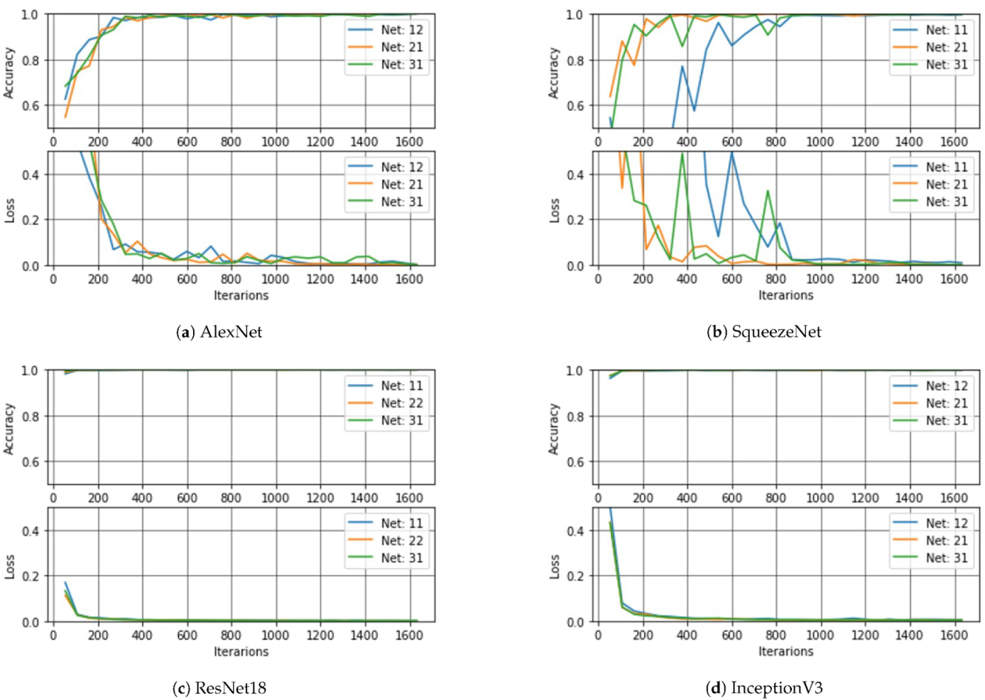
The purpose of this section is to show the impact of the selected net in the performance of the classifier. In this case, nine models were obtained from each network according to the dataset and the freezing point. The three best ones per network were selected to be presented in
Figure 14. The following notation is used for each curve: the first index corresponds to the dataset (i.e., 1 = DS1, 2 = DS2, 3 = DS3), while the second index corresponds to the freezing point (i.e., 1 = UF, 2 = MF, 3 = TF). Thus, if the model is 21, it means that it was trained and validated with DS2, with the freezing point UF. According to the results, the models by transfer learning with AlexNet converge more slowly than those based on the others nets, followed by the models obtained from SqueezeNet. In terms of accuracy and speed of convergence, the best results were obtained with the models by transfer learning with ResNet18.
6.2.2. Impact of the Freezing Point
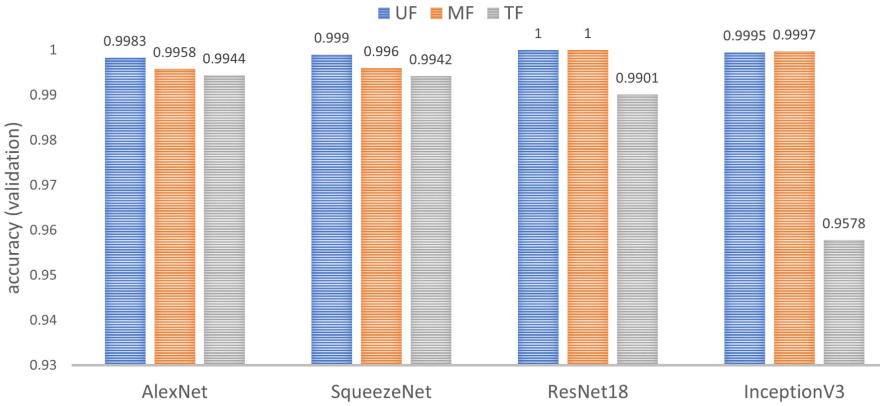
In this test, the impact of the freezing point on the performance of the classifier is considered. For each network, nine models were trained and validated, which were analyzed in terms of
by groups of three models that shared the same freezing point.
Figure 15 shows the consolidated results. In summary, TF is the worst performing point and UF is the best performing point. Furthermore, the network that depends most on the freezing point is InceptionV3.
6.2.3. Impact of the Dataset
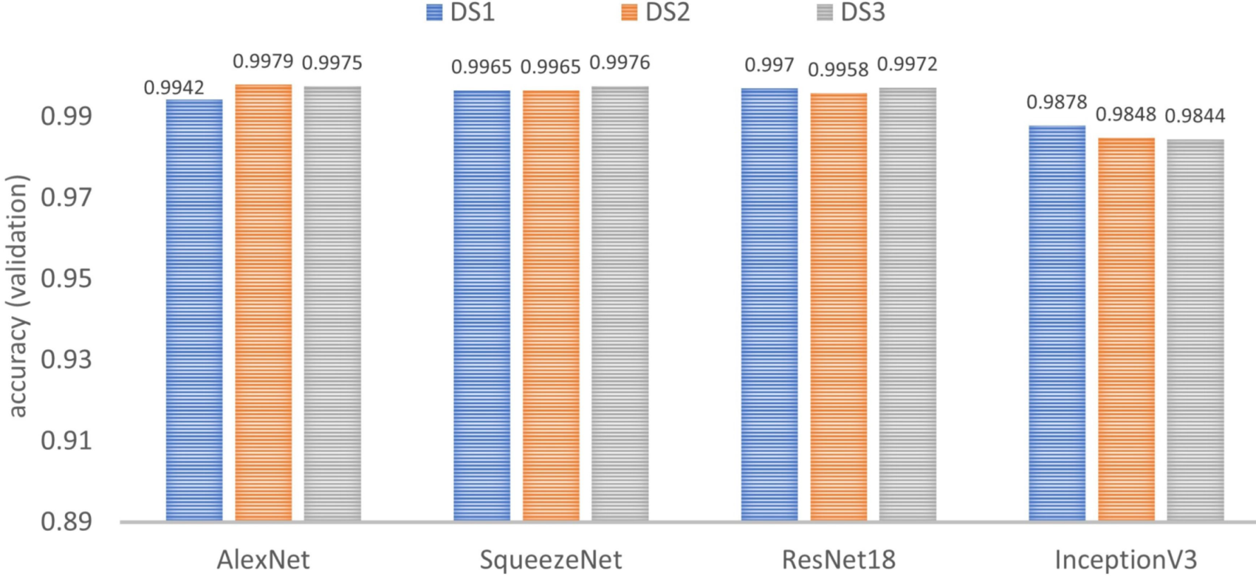
Similar to the previous test, nine models are trained and validated by network, but in this case, they are grouped three by three according to the dataset (see
Figure 16). For all the networks, it is noticeable that the results do not depend significantly on the selected DS. This means that all datasets have good image diversity in all three groups: training, validation and test.
6.3. Custom Model Validation
The Algorithm 1 was also used in the training of the custom model, except for the freezing point.
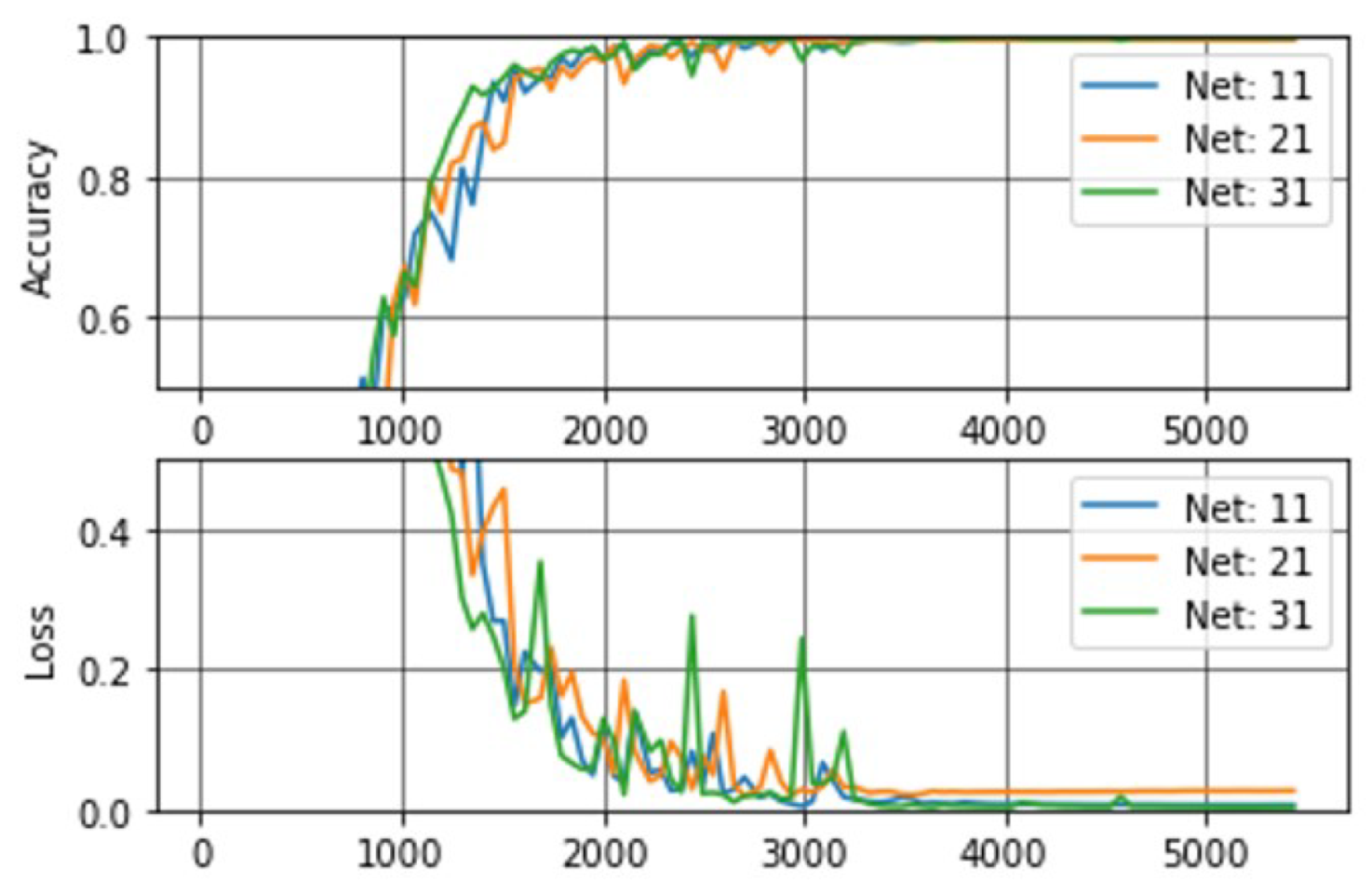
Figure 17 shows the training curves for a total of 10 epochs (i.e., +5000 iterations), where accuracy and loss converge to ideal values as the number of iterations increases. Once again, the independence of the results in relation to the DS used for training is noticeable.
6.4. Comparison between the Proposed Custom Model and the Models by Transfer Learning
The aim of this section is to compare the best model obtained from each pre-trained network with the best model obtained in the custom architecture, in terms of accuracy, inference time, and number of parameters.
6.4.1. Comparison in Terms of Accuracy
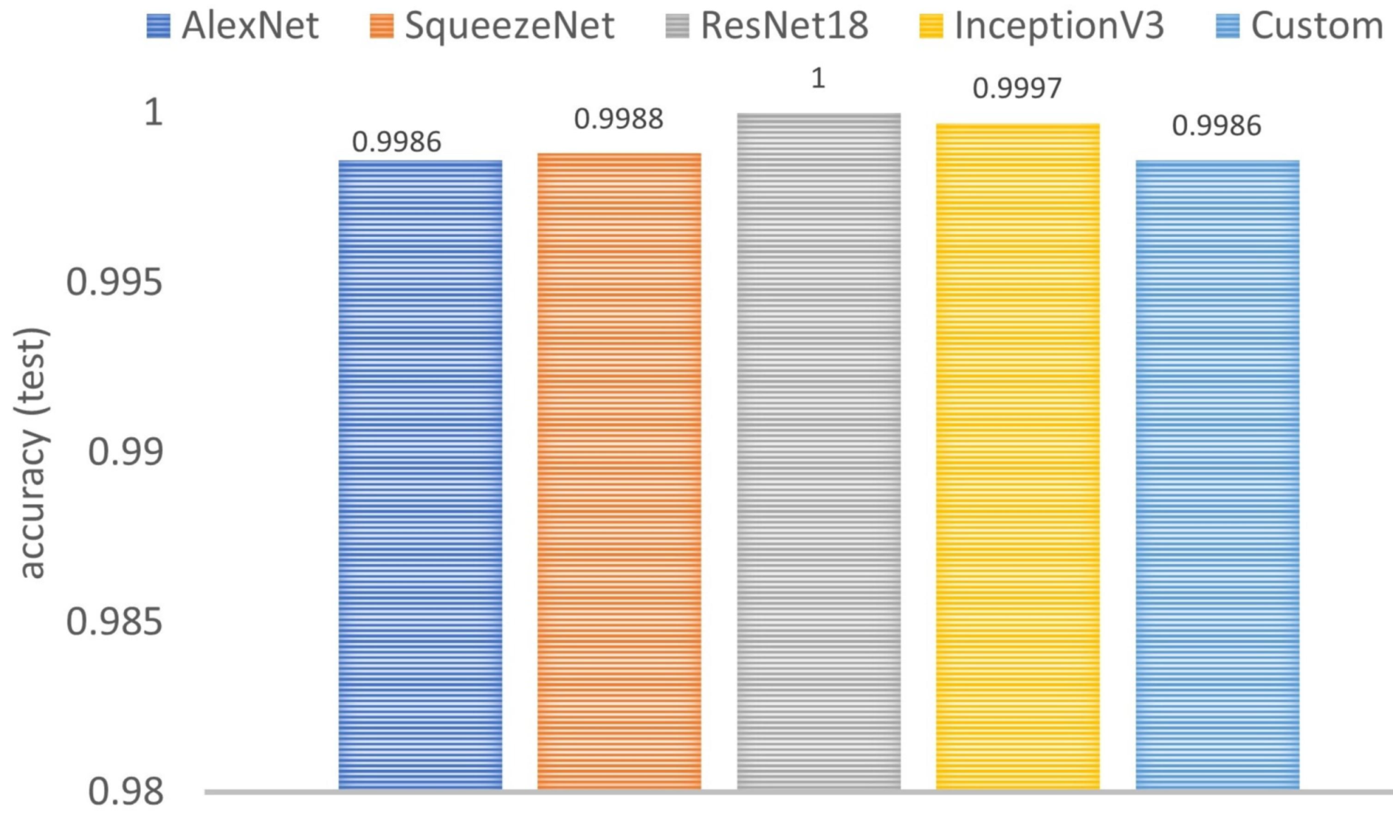
Figure 18 shows the comparison of five models: the custom model from scratch and the four TL-based models. In all cases, the performance is high, since the accuracy is higher than 0.9986. It should be noted that the custom model whose architecture was inspired by AlexNet obtains the same accuracy as that of the model by transfer learning using AlexNet.
6.4.2. Comparison in Terms of the Number of Parameters
Figure 19 shows the results in terms of number of parameters (see
Figure 19a) and file size (see
Figure 19b), which are two important requirements for massive data analysis in low-capacity systems. As expected, these two metrics are closely related. The best model is the one obtained from SqueezNet, followed by the proposed custom model. Our model from scratch is 8× smaller than AlexNet, 3× smaller than InceptionV3 and 1.5× smaller than ResNet18.
6.4.3. Comparison in Terms of Inference Time
Another criterion that was also used in the comparison was the inference time on both CPU (see
Figure 20a) and GPU (see
Figure 20b). When selecting the CPU, the proposed model is the best option because it is faster than its competitors, as follows: 6.48× than InceptionV3, 2.48× than ResNet18, 2.2× than AlexNet and 1.8× than SqueezeNet. In addition, when selecting the CPU, the inference time in the proposed model is very close to AlexNet, 16.3× faster than InceptionV3, 4.2× faster than ResNet18 and 3.1× faster than SqueezeNet.
6.5. Architecture Recommendation
According to the results reported in the previous subsections, there is no model that has the best results in all the comparison criteria, so the following recommendations are made for each criterion,
Accuracy: According to the results, the freezing point TF is not recommended in any of the modelss. It occurs as a consequence of freezing the weights (kernels) of all the layers in the CNNs does not allow them to adjust to the features of the new dataset. Therefore, as a first option, we suggest a model by transfer learning from ResNet18, with freezing point of UF or MF. However, the other models also reported very high accuracy values.
Inference time in CPU: Two factors directly affect inference times. The first corresponds to the number of network parameters, and the second to the complexity of the network. When the number of parameters increases, there is a direct increase in the inference time; while, complex networks with non-sequential operations (such as Inception or ResNet) also increase the inference times in relation to non-complex networks but with a similar amount of parameters. As a result, networks such as Alexnet, ResNet18 and InceptionV3 can be affected by these factors when the inference is performed in CPU. Therefore, as a first option, we suggest the custom model followed by the model obtained from SqueezeNet.
Inference time in GPU: For concatenation operations or addition of tensors, it can take a GPU more time than just performing convolution and pooling operations. Therefore, the more complex the network is (not only its number of parameters), the more time it will take to make inferences per image. Therefore, as a first option, we suggest the custom model followed by the model obtained from AlexNet.
Number of parameters and file size: The file size is related proportionally to the number of network parameters and is not influenced by the type of architecture used. If the device has little storage capacity, we recommend SqueezeNet or the custom model.
6.6. Custom Model vs. State-of-the-Art
Finally, the custom model is compared with some state-of-the-art banknote recognition works in terms of inference time, specifically frames per second (FPS). The results are shown in
Table 4. It can be noted that in terms of CPU inference times, the custom model can analyze a larger amount of images in a shorter period of time, being up to 6.26× faster than the best of the implementations in a Raspberry Pi 3 and up to 17× faster than the one implemented in a computer. On the other hand, in terms of GPU inference times, the proposed model exceeds other networks such as the CNN GoogleNet, which used a Jetson Xavier with better specifications. The proposed custom model was only outperformed by one of the works.
7. Conclusions
This work introduced a comparison between custom models and models by transfer learning in the task of banknote recognition and counterfeit detection. In addition, the impact of the freezing point of models by transfer learning on the performance of the classifier was analyzed, obtaining that unfreezing the weights (UF) or only freezing those of the first half of the network (MF) are the best design alternatives. The proposed custom model was the best in terms of inference times for both CPU and GPU and was very close to being the best in terms of accuracy (i.e., ResNet18). Finally, we present some recommendations to select the most appropriate model for this type of classification task, taking into account different selection criteria.
The design of a custom model in the task of recognizing banknotes and counterfeits, allows it to learn specialized features that help to differentiate between different denominations of banknotes and their corresponding counterfeits. In addition, the custom model can achieve similar results in terms of accuracy compared to those trained by TL and even improve inference times. The main disadvantage of a custom model is the training time and the need for a sufficiently diverse dataset to facilitate its generalization during training.
For future developments, we will seek to apply the same methodology in other datasets of the state-of-the-art, in order to identify if the behavior can be affected according to the distribution of the dataset, architectures to be used, and the established freezing points (FP).
Author Contributions
Conceptualization, C.G.P. and D.M.B.; methodology, C.G.P. and D.M.B. and D.R.; software, C.G.P.; validation, D.M.B. and D.R., C.G.P.; formal analysis, D.M.B.; investigation, D.M.B. and D.R., C.G.P.; data curation, C.G.P. and D.M.B.; writing–original draft preparation, C.G.P.; writing–review and editing, D.M.B. and D.R.; visualization, C.G.P. and D.M.B.; supervision, D.R.; All authors have read and agreed to the published version of the manuscript.
Funding
This research was funded by “Vicerrectoría de Investigaciones—Universidad Militar Nueva Granada”, grant number IMP-ING-2936.
Institutional Review Board Statement
Not applicable.
Informed Consent Statement
Not applicable.
Data Availability Statement
The images of the dataset "Original and counterfeit Colombian peso banknotes" are openly available at [
28] under license CC-BY-4.0.
Conflicts of Interest
The authors declare no conflict of interest.
References
- Lundblad, L.J.; Vedin, L.; Bjorkman, C. Method for a Banknote Detector Device, and a Banknote Detector Device. US Patent 8,942,461, 27 January 2015. [Google Scholar]
- Lee, S.H.; Lee, H.Y. Counterfeit Bill Detection Algorithm using Deep Learning. Int. J. Appl. Eng. Res. 2018, 13, 304–310. [Google Scholar]
- Manikandan, K.; Sumithra, T. Currency recognition in mobile application for visually challenged. Discovery 2015, 30, 245–248. [Google Scholar]
- Youn, S.; Choi, E.; Baek, Y.; Lee, C. Efficient multi-currency classification of CIS banknotes. Neurocomputing 2015, 156, 22–32. [Google Scholar] [CrossRef]
- Cao, B.Q.; Liu, J.X. Currency recognition modeling research based on BP neural network improved by gene algorithm. In Proceedings of the 2010 Second International Conference on Computer Modeling and Simulation, Sanya, China, 22–24 January 2010; Volume 2, pp. 246–250. [Google Scholar] [CrossRef]
- AL-Gawda, M.; Beiji, Z.; Mohammed, N. Yemeni mobile counterfeit detection system using support vector machines, fuzzy logic and image processing techniques. J. Comput. Theor. Nanosci. 2016, 13, 2965–2977. [Google Scholar] [CrossRef]
- Podgorelec, V.; Pečnik, Š.; Vrbančič, G. Classification of Similar Sports Images Using Convolutional Neural Network with Hyper-Parameter Optimization. Appl. Sci. 2020, 10, 8494. [Google Scholar] [CrossRef]
- Hameed, K.; Chai, D.; Rassau, A. A Sample Weight and AdaBoost CNN-Based Coarse to Fine Classification of Fruit and Vegetables at a Supermarket Self-Checkout. Appl. Sci. 2020, 10, 8667. [Google Scholar] [CrossRef]
- Ulloa, C.; Ballesteros, D.M.; Renza, D. Video Forensics: Identifying Colorized Images Using Deep Learning. Appl. Sci. 2021, 11, 476. [Google Scholar] [CrossRef]
- Krizhevsky, A.; Sutskever, I.; Hinton, G.E. Imagenet classification with deep convolutional neural networks. Commun. ACM 2017, 60, 84–90. [Google Scholar] [CrossRef]
- He, K.; Zhang, X.; Ren, S.; Sun, J. Deep Residual Learning for Image Recognition. In Proceedings of the IEEE Conference on Computer Vision and Pattern Recognition (CVPR), Las Vegas, NV, USA, 27–30 June 2016. [Google Scholar]
- Berenguel, A.; Terrades, O.R.; Lladós i, J.; Cañero, C. Evaluation of Texture Descriptors for Validation of Counterfeit Documents. In Proceedings of the 2017 14th IAPR International Conference on Document Analysis and Recognition (ICDAR), Las Vegas, NV, USA, 27–30 June 2017; Volume 1, pp. 1237–1242. [Google Scholar] [CrossRef]
- Galeana Pérez, D.; Bayro Corrochano, E. Recognition system for euro and Mexican banknotes based on deep learning with real scene images. Comput. Sist. 2018, 22, 1065–1076. [Google Scholar] [CrossRef]
- Park, C.; Cho, S.W.; Baek, N.R.; Choi, J.; Park, K.R. Deep Feature-Based Three-Stage Detection of Banknotes and Coins for Assisting Visually Impaired People. IEEE Access 2020, 8, 184598–184613. [Google Scholar] [CrossRef]
- Pham, T.D.; Park, C.; Nguyen, D.T.; Batchuluun, G.; Park, K.R. Deep Learning-Based Fake-Banknote Detection for the Visually Impaired People Using Visible-Light Images Captured by Smartphone Cameras. IEEE Access 2020, 8, 63144–63161. [Google Scholar] [CrossRef]
- Kuo, C.C.J. Understanding convolutional neural networks with a mathematical model. J. Vis. Commun. Image Represent. 2016, 41, 406–413. [Google Scholar] [CrossRef]
- Goodfellow, I.; Bengio, Y.; Courville, A.; Bengio, Y. Deep Learning; MIT Press: Cambridge, UK, 2016; Volume 1. [Google Scholar]
- Zeiler, M.D.; Fergus, R. Visualizing and Understanding Convolutional Networks. In Computer Vision—ECCV 2014; Fleet, D., Pajdla, T., Schiele, B., Tuytelaars, T., Eds.; Springer International Publishing: Cham, Switzerland, 2014; pp. 818–833. [Google Scholar] [CrossRef]
- LeCun, Y.; Bengio, Y.; Hinton, G. Deep learning. Nature 2015, 521, 436–444. [Google Scholar] [CrossRef]
- Lecun, Y.; Bottou, L.; Bengio, Y.; Haffner, P. Gradient-based learning applied to document recognition. Proc. IEEE 1998, 86, 2278–2324. [Google Scholar] [CrossRef]
- LeNail, A. Nn-svg: Publication-ready neural network architecture schematics. J. Open Source Softw. 2019, 4, 747. [Google Scholar] [CrossRef]
- Szegedy, C.; Liu, W.; Jia, Y.; Sermanet, P.; Reed, S.; Anguelov, D.; Erhan, D.; Vanhoucke, V.; Rabinovich, A. Going Deeper with Convolutions. In Proceedings of the IEEE Conference on Computer Vision and Pattern Recognition (CVPR), Boston, MA, USA, 7–12 June 2015. [Google Scholar]
- Deng, J.; Dong, W.; Socher, R.; Li, L.; Li, K.; Li, F.-F. ImageNet: A large-scale hierarchical image database. In Proceedings of the 2009 IEEE Conference on Computer Vision and Pattern Recognition, Miami, FL, USA, 20–25 June 2009; pp. 248–255. [Google Scholar] [CrossRef]
- Lin, T.Y.; Maire, M.; Belongie, S.; Hays, J.; Perona, P.; Ramanan, D.; Dollár, P.; Zitnick, C.L. Microsoft COCO: Common Objects in Context. In Computer Vision–ECCV 2014; Fleet, D., Pajdla, T., Schiele, B., Tuytelaars, T., Eds.; Springer International Publishing: Cham, Switzerland, 2014; pp. 740–755. [Google Scholar]
- Zhuang, F.; Qi, Z.; Duan, K.; Xi, D.; Zhu, Y.; Zhu, H.; Xiong, H.; He, Q. A Comprehensive Survey on Transfer Learning. Proc. IEEE 2021, 109, 43–76. [Google Scholar] [CrossRef]
- Baek, S.; Choi, E.; Baek, Y.; Lee, C. Detection of counterfeit banknotes using multispectral images. Digit. Signal Process. 2018, 78, 294–304. [Google Scholar] [CrossRef]
- Perez, L.; Wang, J. The effectiveness of data augmentation in image classification using deep learning. arXiv 2017, arXiv:1712.04621. [Google Scholar]
- Pachon Suescun, C.G.; Ballesteros L, D.M.; Renza, D. Original and counterfeit Colombian peso banknotes. Mendeley Data V2 2021. [Google Scholar] [CrossRef]
- Bonafilia, D.; Tellman, B.; Anderson, T.; Issenberg, E. Sen1Floods11: A georeferenced dataset to train and test deep learning flood algorithms for Sentinel-1. In Proceedings of the IEEE/CVF Conference on Computer Vision and Pattern Recognition (CVPRW) Workshops, Seattle, WA, USA, 14–19 June 2020; pp. 835–845. [Google Scholar] [CrossRef]
- Gurpinar, F.; Kaya, H.; Dibeklioglu, H.; Salah, A. Kernel ELM and CNN Based Facial Age Estimation. In Proceedings of the IEEE Conference on Computer Vision and Pattern Recognition (CVPR) Workshops, Las Vegas, NV, USA, 26 June–1 July 2016. [Google Scholar]
- Shin, H.; Roth, H.R.; Gao, M.; Lu, L.; Xu, Z.; Nogues, I.; Yao, J.; Mollura, D.; Summers, R.M. Deep Convolutional Neural Networks for Computer-Aided Detection: CNN Architectures, Dataset Characteristics and Transfer Learning. IEEE Trans. Med. Imaging 2016, 35, 1285–1298. [Google Scholar] [CrossRef] [PubMed]
- Iandola, F.N.; Han, S.; Moskewicz, M.W.; Ashraf, K.; Dally, W.J.; Keutzer, K. SqueezeNet: AlexNet-level accuracy with 50x fewer parameters and <0.5 MB model size. arXiv 2016, arXiv:1602.07360. [Google Scholar]
- Szegedy, C.; Vanhoucke, V.; Ioffe, S.; Shlens, J.; Wojna, Z. Rethinking the Inception Architecture for Computer Vision. In Proceedings of the IEEE Conference on Computer Vision and Pattern Recognition (CVPR), Las Vegas, NV, USA, 27–30 June 2016. [Google Scholar]
- Joulin, A.; Cissé, M.; Grangier, D.; Jégou, H. Efficient softmax approximation for gpus. In Proceedings of the International Conference on Machine Learning (PMLR), Sydney, Australia, 6–1 August 2017; pp. 1302–1310. [Google Scholar]
- Glorot, X.; Bengio, Y. Understanding the difficulty of training deep feedforward neural networks. In Proceedings of the Thirteenth International Conference on Artificial Intelligence and Statistics, Sardinia, Italy, 13–15 May 2010; pp. 249–256. [Google Scholar]
- Bergstra, J.; Bengio, Y. Random search for hyper-parameter optimization. J. Mach. Learn. Res. 2012, 13, 281–305. [Google Scholar]
- Torres, J.F.; Gutiérrez-Avilés, D.; Troncoso, A.; Martínez-Álvarez, F. Random hyper-parameter search-based deep neural network for power consumption forecasting. In International Work-Conference on Artificial Neural Networks; Springer: Cham, Switzerland, 2019; pp. 259–269. [Google Scholar] [CrossRef]
- Dunai Dunai, L.; Chillarón Pérez, M.; Peris-Fajarnés, G.; Lengua Lengua, I. Euro banknote recognition system for blind people. Sensors 2017, 17, 184. [Google Scholar] [CrossRef]
- Ayalew Tessfaw, E.; Ramani, B.; Kebede Bahiru, T. Ethiopian Banknote Recognition and Fake Detection Using Support Vector Machine. In Proceedings of the 2018 Second International Conference on Inventive Communication and Computational Technologies (ICICCT), Coimbatore, India, 20–21 April 2018; pp. 1354–1359. [Google Scholar] [CrossRef]
- Moreno H, G.A.; Forero, M.G.; Tamayo Z, K. Banknotes classification system through image processing and pattern recognition for people with visual impairment. In Proceedings of the Applications of Digital Image Processing XLII, San Diego, CA, USA, 11–15 August 2019. [Google Scholar] [CrossRef]
- Han, M.; Kim, J. Joint banknote recognition and counterfeit detection using explainable artificial intelligence. Sensors 2019, 19, 3607. [Google Scholar] [CrossRef]
- Hasanuzzaman, F.M.; Yang, X.; Tian, Y. Robust and Effective Component-Based Banknote Recognition for the Blind. IEEE Trans. Syst. Man Cybern. Syst. Part C (Appl. Rev.) 2012, 42, 1021–1030. [Google Scholar] [CrossRef]
Figure 1.
Example of a sequential convolutional neural network (CNN) architecture. The figure was generated using NN-SVG [
21].
Figure 1.
Example of a sequential convolutional neural network (CNN) architecture. The figure was generated using NN-SVG [
21].
Figure 2.
Example of a residual CNN architecture. The figure was generated using NN-SVG [
21].
Figure 2.
Example of a residual CNN architecture. The figure was generated using NN-SVG [
21].
Figure 3.
Example of inception module in CNN architectures.
Figure 3.
Example of inception module in CNN architectures.
Figure 4.
Example of transfer Learning in a sequential CNN by replacing the last layer. Numbers in square brackets correspond to [Channels × Height × Width]. It was generated using NN-SVG [
21].
Figure 4.
Example of transfer Learning in a sequential CNN by replacing the last layer. Numbers in square brackets correspond to [Channels × Height × Width]. It was generated using NN-SVG [
21].
Figure 5.
Proposed capture module for the detection of denominations and counterfeit banknotes using a CNN.
Figure 5.
Proposed capture module for the detection of denominations and counterfeit banknotes using a CNN.
Figure 6.
Examples of images of Colombian banknotes. Available at [
28] under license CC-BY-4.0.
Figure 6.
Examples of images of Colombian banknotes. Available at [
28] under license CC-BY-4.0.
Figure 7.
Characteristics of the dataset used (Colombian banknotes): number of images, image distribution and classes.
Figure 7.
Characteristics of the dataset used (Colombian banknotes): number of images, image distribution and classes.
Figure 8.
Image distribution in each of the datasets (DS).
Figure 8.
Image distribution in each of the datasets (DS).
Figure 9.
Transfer learning options. UF (not frozen weights), MF (medium freezing point), TF (totally frozen, except for the last fully connected (FC) layer). The image was generated using NN-SVG [
21].
Figure 9.
Transfer learning options. UF (not frozen weights), MF (medium freezing point), TF (totally frozen, except for the last fully connected (FC) layer). The image was generated using NN-SVG [
21].
Figure 10.
Proposed network for the task of fake banknote recognition, (S:Stride). The figure was generated using NN-SVG [
21].
Figure 10.
Proposed network for the task of fake banknote recognition, (S:Stride). The figure was generated using NN-SVG [
21].
Figure 11.
Comparison between training the custom model with randomized weight initialization or Xavier method.
Figure 11.
Comparison between training the custom model with randomized weight initialization or Xavier method.
Figure 12.
Example of feature maps for some banknotes (original and fake).
Figure 12.
Example of feature maps for some banknotes (original and fake).
Figure 13.
Examples of feature maps for original banknotes.
Figure 13.
Examples of feature maps for original banknotes.
Figure 14.
Convergence comparison for different TL-based models. The first index in each network corresponds to the dataset (i.e., 1 = DS1, 2 = DS2, 3 = DS3), while the second index corresponds to the freezing point (i.e., 1 = UF, 2 = MF, 3 = TF).
Figure 14.
Convergence comparison for different TL-based models. The first index in each network corresponds to the dataset (i.e., 1 = DS1, 2 = DS2, 3 = DS3), while the second index corresponds to the freezing point (i.e., 1 = UF, 2 = MF, 3 = TF).
Figure 15.
Comparison of four TL-based models in terms of Freezing Point. UF (not frozen weights), MF (medium freezing point), TF (totally frozen, except for the last FC layer).
Figure 15.
Comparison of four TL-based models in terms of Freezing Point. UF (not frozen weights), MF (medium freezing point), TF (totally frozen, except for the last FC layer).
Figure 16.
Comparison of four TL-based models in terms of dataset organization (DS1, DS2, DS3).
Figure 16.
Comparison of four TL-based models in terms of dataset organization (DS1, DS2, DS3).
Figure 17.
Accuracy and loss graphs during custom model trainings. The first index in each network corresponds to the dataset (i.e., 1 = DS1, 2 = DS2, 3 = DS3), while the second index corresponds to the freezing point (i.e., 1 = UF, 2 = MF, 3 = TF).
Figure 17.
Accuracy and loss graphs during custom model trainings. The first index in each network corresponds to the dataset (i.e., 1 = DS1, 2 = DS2, 3 = DS3), while the second index corresponds to the freezing point (i.e., 1 = UF, 2 = MF, 3 = TF).
Figure 18.
Comparison of the custom model and the four TL-based models in terms of accuracy (the higher the better).
Figure 18.
Comparison of the custom model and the four TL-based models in terms of accuracy (the higher the better).
Figure 19.
Comparison of the custom model and the four TL-based models in terms of number of parameters and in terms of file size.
Figure 19.
Comparison of the custom model and the four TL-based models in terms of number of parameters and in terms of file size.
Figure 20.
Comparison of the custom model and the four TL-based models in terms of CPU and GPU inference time.
Figure 20.
Comparison of the custom model and the four TL-based models in terms of CPU and GPU inference time.
Table 1.
Summary of the proposed network (K: Kernel, S: Stride, P: Padding).
Table 1.
Summary of the proposed network (K: Kernel, S: Stride, P: Padding).
| Layer | No. of Filters | K | S | P | Output Shape | Trainable Parameters |
|---|
| Input | - | - | - | - | (224, 224, 3) | 0 |
| Conv-1 | 64 | 11 | 4 | 2 | (55, 55, 64) | 23,296 |
| ReLu | - | - | - | - | (55, 55, 64) | 0 |
| MaxPooling-1 | 64 | 3 | 2 | 0 | (27, 27, 64) | 0 |
| Conv-2 | 192 | 5 | 1 | same | (27, 27, 192) | 307,392 |
| ReLu | - | - | - | - | (27, 27, 192) | 0 |
| MaxPooling-2 | 192 | 3 | 2 | 0 | (13, 13, 192) | 0 |
| Conv-3 | 384 | 3 | 1 | same | (13, 13, 384) | 663,936 |
| ReLu | - | - | - | - | (13, 13, 384) | 0 |
| Conv-4 | 256 | 3 | 1 | same | (13, 13, 256) | 884,992 |
| ReLu | - | - | - | - | (13, 13, 256) | 0 |
| Conv-5 | 256 | 3 | 1 | same | (13, 13, 256) | 590,080 |
| ReLu | - | - | - | - | (13, 13, 256) | 0 |
| MaxPooling-3 | 256 | 3 | 2 | 0 | (6, 6, 256) | 0 |
| Adaptative Pooling 6 × 6 | - | - | - | - | (6, 6, 256) | 0 |
| Flattening | - | - | - | - | (9216, 1) | 0 |
| Dropout 0.5 | - | - | - | - | (9216, 1) | 0 |
| FC-1 | 512 | - | - | - | (512, 1) | 4, 719,104 |
| Dropout 0.5 | - | - | - | - | (512, 1) | 0 |
| FC-2 | 512 | - | - | - | (512, 1) | 262,656 |
| FC-3 | 13 | - | - | - | (13, 1) | 6669 |
| Softmax/Classification |
| | | | | | Total parameters: | 7,458,125 |
Table 2.
Hyperparameters of the training stage: transfer leaning (TL)-based models and custom model.
Table 2.
Hyperparameters of the training stage: transfer leaning (TL)-based models and custom model.
| Batch Size | Epoch | Optimizer | Momentum | Learning Rate | Loss |
|---|
| 24 | 3/10 | SGDM | 0.9 | 0.003 | Cross-Entropy |
Table 3.
Hardware specifications for the training and inference stages.
Table 3.
Hardware specifications for the training and inference stages.
| Device | RAM | CPU | GPU |
|---|
| Computer | 16 GB DDR4 | Core i7-6700HQ | NVIDIA® GeForce® GTX 960M/640 Cuda Cores |
| Jetson Nano | 4 GB DDR4 | Quad-core ARM® A57 | 128-core NVIDIA Maxwell™ architecture |
Table 4.
Comparison of the proposed model with similar systems in the state-of-the-art.
Table 4.
Comparison of the proposed model with similar systems in the state-of-the-art.
| Research | Method | CPU (FPS) | GPU (FPS) | Hardware |
|---|
| [38] | Haar techniques | 0.11–0.07 | – | Raspberry Pi 3 |
| [39] | Support Vector Machine | 0.16 | – | |
| [40] | Neural Networks (MLP) | 1.1 | – | |
| | CNN GoogleNet | – | 123.15 | Jetson Xavier |
| [41] | Two sequential neural networks | – | 1.05 | |
| | CNN with Gaussian smoothing operator | – | 229.35 | |
| [42] | SURF descriptors | 0.4 | - | PC with 3-GHz CPU |
| Proposed custom model | Sequential CNN | 6.89 | 185.18 | Jetson Nano |
| Publisher’s Note: MDPI stays neutral with regard to jurisdictional claims in published maps and institutional affiliations. |
© 2021 by the authors. Licensee MDPI, Basel, Switzerland. This article is an open access article distributed under the terms and conditions of the Creative Commons Attribution (CC BY) license (http://creativecommons.org/licenses/by/4.0/).
