Article

Learning to Localise Automated Vehicles in Challenging Environments Using Inertial Navigation Systems (INS)

1
Institute for Future Transport and Cities, Coventry University, Gulson Road, Coventry CV1 5FB, UK
2
Research Centre for Data Science, Coventry University, Priory Road, Coventry CV1 5FB, UK
3
Faculty of Engineering, Coventry University, Priory Road, Coventry CV1 5 FB, UK
*
Author to whom correspondence should be addressed.
Appl. Sci. 2021, 11(3), 1270; https://doi.org/10.3390/app11031270
Submission received: 21 December 2020 / Revised: 19 January 2021 / Accepted: 25 January 2021 / Published: 30 January 2021
(This article belongs to the Special Issue Artificial Intelligence for Connected and Automated Vehicles)

Abstract

:
An approach based on Artificial Neural Networks is proposed in this paper to improve the localisation accuracy of Inertial Navigation Systems (INS)/Global Navigation Satellite System (GNSS) based aided navigation during the absence of GNSS signals. The INS can be used to continuously position autonomous vehicles during GNSS signal losses around urban canyons, bridges, tunnels and trees, however, it suffers from unbounded exponential error drifts cascaded over time during the multiple integrations of the accelerometer and gyroscope measurements to position. More so, the error drift is characterised by a pattern dependent on time. This paper proposes several efficient neural network-based solutions to estimate the error drifts using Recurrent Neural Networks, such as the Input Delay Neural Network (IDNN), Long Short-Term Memory (LSTM), Vanilla Recurrent Neural Network (vRNN), and Gated Recurrent Unit (GRU). In contrast to previous papers published in literature, which focused on travel routes that do not take complex driving scenarios into consideration, this paper investigates the performance of the proposed methods on challenging scenarios, such as hard brake, roundabouts, sharp cornering, successive left and right turns and quick changes in vehicular acceleration across numerous test sequences. The results obtained show that the Neural Network-based approaches are able to provide up to 89.55% improvement on the INS displacement estimation and 93.35% on the INS orientation rate estimation.

1. Introduction

The safe navigation of autonomous vehicles and robots alike is dependent on fast and accurate positioning solutions. Autonomous vehicles are commonly localised within a lane using sensors such as cameras, LIDARS and radars, whilst road localisation is achieved through the use of information provided by a Global Navigation Satellite System (GNSS). There are, however, times when the LIDAR or/and camera might be unavailable for use [1,2]. The GNSS, which operates through the trilateration of signals obtained from at least three satellites, is also unreliable. The accuracy of the GNSS deteriorates due to multi-path reflections and visibility issues under bridges and trees, in tunnels and urban canyons [3]. An Inertial Navigation System (INS) can be used to estimate the position and orientation of the vehicle during the GNSS outage periods provided the availability of initial orientation information [4]. Nevertheless, the INS, which is made up of sensors such as the accelerometer and gyroscope, suffers from an exponential error-drift during the double integration of the accelerometer’s measurement to position and the integration of the gyroscopes attitude rate to orientation [5]. These errors are cascaded unboundedly over time to provide a poor positioning solution within the navigation time window [5]. A common approach towards reducing the error drifts involves calibrating the INS periodically with the GNSS. The challenge, therefore, becomes one of accurately predicting the position of the vehicle in the absence of the GNSS signal needed for positioning and correction. Traditionally, Kalman filters are used in modelling the error between the Global Positioning System (GPS) and INS positions [6,7,8]. However, they have limitations when modelling highly non-linear dependencies, stochastic relationships and non-Gaussian noise measurements [6].
Over the years, other methods based on artificial intelligence have been proposed by a number of researchers to learn the error-drift within the sensors’ measurements [9,10,11,12,13,14]. The use of the sigma pi neural network on the positioning problem was explored by Malleswaran et al. in Reference [15]. Noureldin et al. investigated the use of the Input Delay Neural Network (IDNN) to model the INS/GPS positional error [6]. A Multi-Layer Feed-Forward Neural Network (MFNN) was applied in Reference [16] on a single point positioning INS/GPS integrated architecture. Reference [17] employed the MFNN on an integrated tactical grade INS and a Differential GPS architecture for a better position estimation solution. More so, Recurrent Neural Networks, which are distinguishable from other neural networks due to their ability to make nodal connections in temporal sequences, have been proven to model the time-dependent error drift of the INS more accurately compared to other neural network techniques [18]. In Reference [19], Fang et al. compared the performance of the Long Short-Term Memory (LSTM) algorithm to the Multi-Layer Perceptron (MLP) and showed the superiority of the LSTM over the MLP. Similarly, in Reference [1], Onyekpe et al. investigated the performance of the LSTM algorithm for high data rate positioning and compared it to other techniques, such as the IDNN, MLP and Kalman filter.
Nevertheless, we observe that despite the number of techniques investigated on the INS/GPS error drift modelling, there lacks an investigation into the performances of the techniques on complex driving scenarios and environments experienced in everyday driving. Such scenarios range from hard brakes on regular, wet, or muddy roads to sharp cornering scenarios, heavy traffic, roundabouts, etc. We thus set out to investigate the performances of neural network-based approaches on such complex driving environments and show that these scenarios prove rather more challenging for the INS. We propose an approach based on neural networks with inspiration drawn from the operation of the feedback control system, in order to improve the estimation of the neural networks (NN) for the short-term tracking of the vehicles’ displacement in these scenarios.
The rest of the paper is structured as follows. In Section 2, we describe the challenging navigation problem, formulate the inertial navigation mathematical model and describe the structure of the proposed NN approach. In Section 3, we describe the Inertia and Odometry Vehicle Navigation Dataset (IO-VNBD) used as well as the setup of the experiment. In addition, we also define the metrics used to evaluate the performance of the NN technique and furthermore perform a comparative analysis of the IDNN, LSTM, Gated Recurrent Unit (GRU), Vanilla Recurrent Neural Network (vRNN) and MLP in terms of accuracy and computational efficiency. In Section 4, we discuss the results obtained and we conclude our work in Section 5.

2. Problem Description and Formulation (INS Motion Model)

Most of the previous research on vehicle positioning does not take into consideration complex scenarios such as hard brake, sharp cornering or roundabouts. Hence, the evaluation of the performance of positioning algorithms present in most published works may not accurately reflect real-life vehicular driving experience. Moreover, as those complex scenarios present strong challenges for INS tracking, it seems essential for the reliability of the algorithms to be assessed under such scenarios:
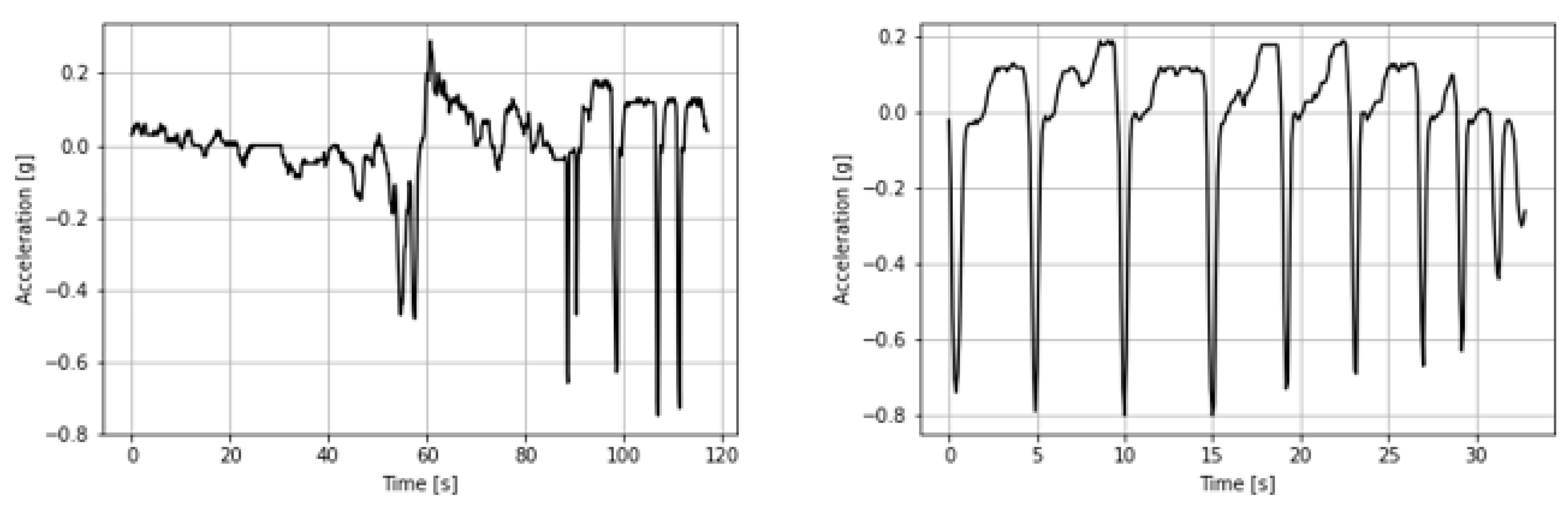
  • Hard brake—According to Reference [20], hard brakes are characterised by a longitudinal deceleration of ≤−0.45 g. They occur when the brake pad of the vehicle has a large force applied to it. The sudden halt to the motion of the vehicle leads to a steep decline in the velocity of the vehicle, thus making it difficult to predict the vehicle coming to a stop and to track the motion of the vehicle thereafter. This scenario poses a major challenge to the displacement estimation of the vehicle.
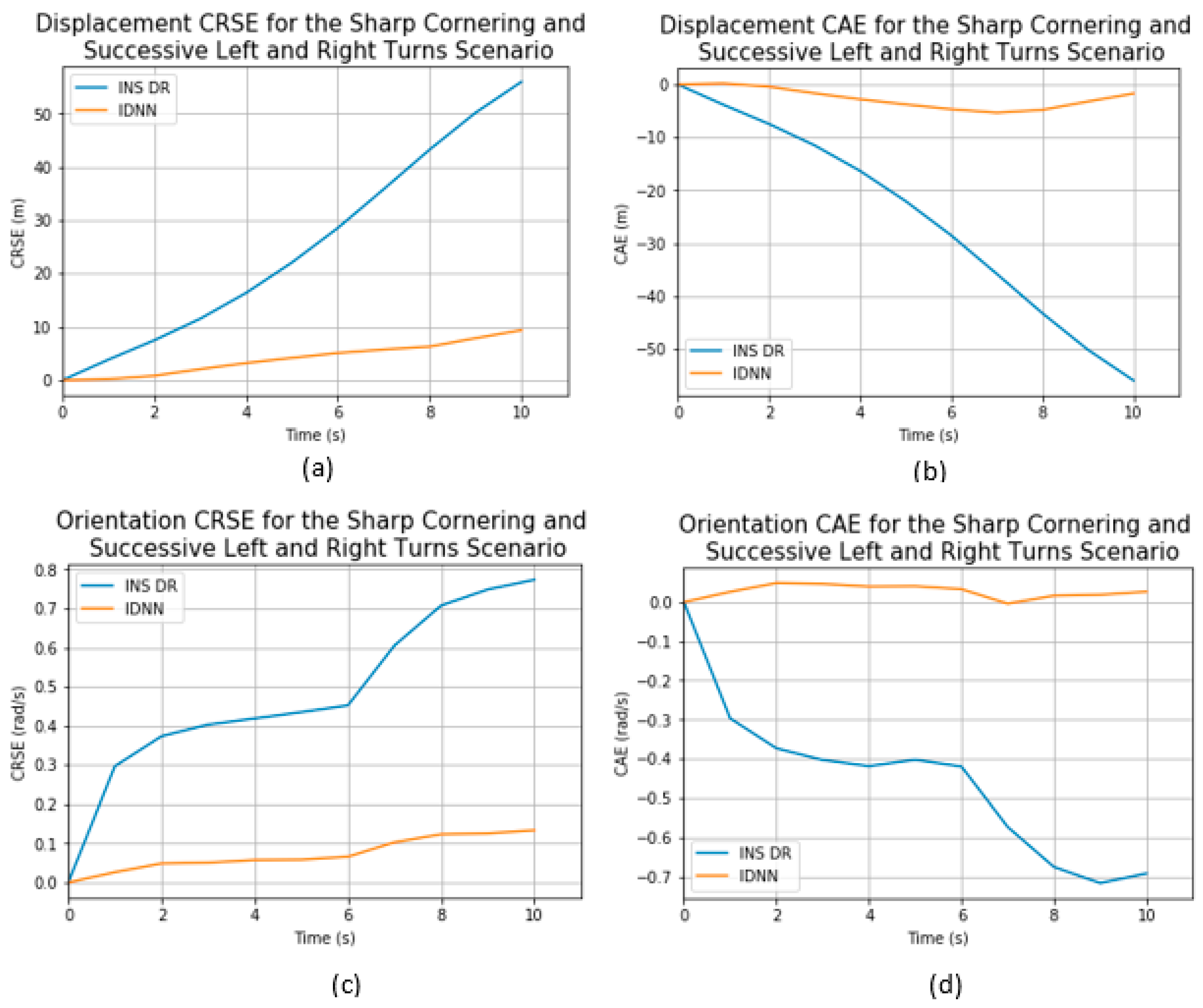
  • Sharp cornering and successive left and right turn—The sudden and consecutive change in the direction of the vehicle also poses a challenge to the orientation estimation of the vehicle. The INS struggles to accurately capture the sudden sharp changes to the orientation of the vehicle as well as continuous consecutive changes to the vehicle in relatively short periods of time.
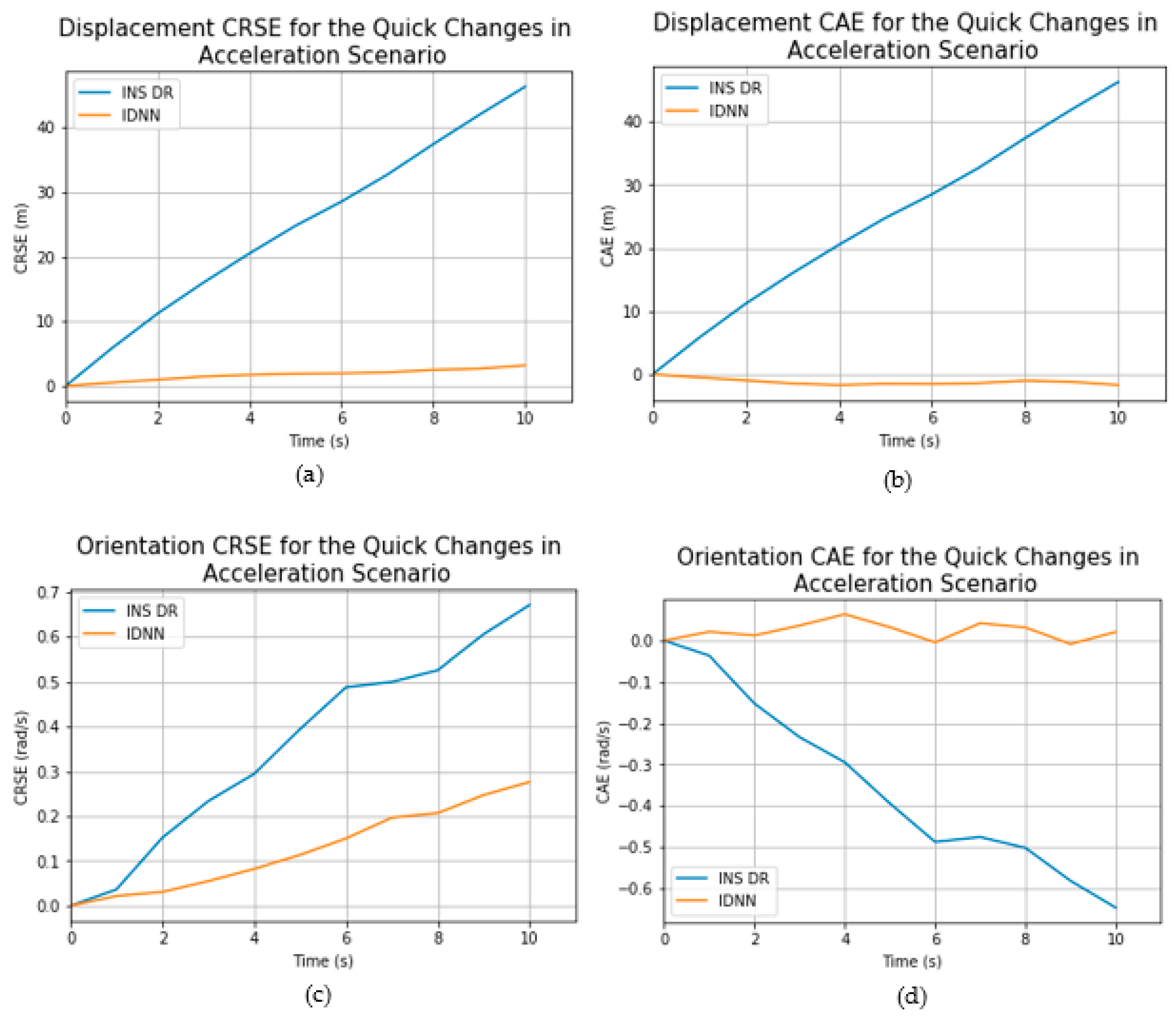
  • Changes in acceleration (Jerk)—The accuracy of the displacement estimation of the INS is affected by quick and varied changes to the acceleration of the vehicle within a short period of time. This is particularly a challenge as the INS struggles to capture the quick change in the vehicle’s displacement thereafter.
  • Roundabout—Roundabouts present a particular struggle due to its shape. The circular and unidirectional traffic flow makes it a challenge to track the vehicle’s orientation and displacement particularly due to the continuous change in the vehicle’s direction whilst navigating the roundabout. Different roundabout sizes were considered in this study.

2.1. INS/GNSS Motion Model

Tracking the position of a vehicle is usually done relative to a reference. The INS’s measurements usually provided in the body (sensors) frame would need to be transformed into the navigation frame for tracking purposes [21]. In this study, we adopt the North-East-Down convention in defining the navigation frame. The transformation matrix R n b from the body frame to navigation frame is as shown in Equation   ( 1 )
R n b = [ c o s θ c o s Ψ   c o s θ   s i n Ψ + s i n ϕ   s i n θ   c o s Ψ s i n ϕ   s i n Ψ + c o s ϕ   s i n θ   c o s Ψ c o s θ   s i n Ψ     c o s ϕ   c o s Ψ +   s i n ϕ   s i n θ   s i n Ψ s i n ϕ   c o s Ψ + c o s ϕ   s i n θ   s i n Ψ s i n θ s i n ϕ c o s θ c o s ϕ c o s θ   ] .
where ϕ is the roll, θ is the pitch and Ψ is the yaw. However, as our study is limited to the two-dimensional tracking of vehicles, ϕ and θ are thus considered to be zero, thus the rotation matrix R n b   becomes:
R n b = [ c o s Ψ   s i n Ψ 0 s i n Ψ     c o s Ψ 0 0 0 1 ]
The gyroscope measures the rate of change of attitude (angular velocity) in yaw, roll and pitch with respect to the inertial frame as expressed in the body frame [1,21]. Giving initial orientation information Ψ 0 , the attitude rate ω b can be integrated to provide continuous orientation Ψ I N S information in the absence of the GNSS signal.
Ψ I N S = Ψ 0 + t 1 t ω b
The accelerometer measures the specific force (In the vehicle tracking application, the centrifugal acceleration is considered absorbed in the local gravity sector and the centrifugal acceleration considered negligible due to its small magnitude.) f b on the sensor in the body frame and is as expressed in Equation (4); where g n represents the gravity vector, R b n is the rotation matrix from the navigation frame to the body frame and a n denotes the linear acceleration of the sensor expressed in the navigation frame.
f b = R b n ( a n g n )
However, the accelerometer measurements at each time t are usually corrupted by a bias δ I N S b and noise ε a b , and is thus represented by F I N S b , as shown in Equation   ( 5 ) .
F I N S b = f I N S b + δ I N S b + ε a b
More so, the accelerometer’s bias varies slowly with time and as such can be modelled as a constant parameter; whilst the accelerometer’s noise is somewhat characterised by a Gaussian distribution and modelled as ε a b ~ N ( 0 , Σ a ) . Therefore, the specific measurement equation as expressed in Equation (4) can be expanded as shown below, where a b is the linear acceleration in the body frame and g b is the gravity vector in the body frame.
from   Equation   ( 4 ) ,   a b = f b + g b ,
from   Equation   ( 5 ) ,    F I N S b = a I N S b + δ I N S ,   a b + ε a b
a b = F I N S b δ I N S ,   a b ε   a b
a b + ε a b =   F I N S b δ I N S ,   a b
However ,   a I N S b = F I N S b δ I N S ,   a b
a I N S b = a b + ε a b
where a I N S b is the bias and gravity compensated acceleration measurement. The vehicle’s velocity in the body frame can be estimated through the integration of Equation   ( 11 ) as shown below:
v I N S b = t 1 t a b + ε v b
Through the double integration of Equation   ( 11 ) , the displacement of the vehicle in the body frame at time t from t 1 , x I N S b , can also be determined as shown in Equation   ( 13 ) .
x I N S b = t 1 t a b + ε   x b
where ε   x b and ε   v b are the noise characterising the INS’s displacement and velocity information formulation derived from ε   a b , δ I N S ,   a b is the sensors bias in the body frame calculated as a constant parameter from the average reading of a stationary accelerometer ran for 20 min, F I N S b is the corrupted measurement of the accelerometer sensor at time t (sampling time), g is the gravity vector and t 1 t a b , t 1 t a b and a b are the uncorrupted (true) displacement, velocity and acceleration, respectively, of the vehicle.
Thus, the vehicle’s true displacement is expressed as x G N S S b t 1 t a b .
Furthermore, ε   x b can be obtained by:
ε   x b   x G N S S b   x I N S b
Using the North-East-Down (NED) system, the noise ε   x b , displacement x I N S b , velocity v I N S b and acceleration a I N S b of the vehicle in the body frame within the window t 1 to t can be transformed into the navigation frame using R n b as shown in Equations (15)–(19). However, the down axis is not considered in this study. More so, the window size in this study is defined as 1 s.
R I N S n b   .   a I N S b       a I N S n   a I N S b   .   c o s Ψ ,   a I N S b   .   s i n Ψ ,
R I N S n b   .   v I N S b   v I N S n   v I N S b   .   c o s Ψ I N S ,   v I N S b   .   s i n Ψ ,
R I N S n b   .   x I N S b     x I N S n   x I N S b   .   c o s Ψ ,   x I N S b   .   s i n Ψ ,
Where :   R I N S n b = [ c o s Ψ I N S   s i n Ψ I N S 0 s i n Ψ I N S     c o s Ψ I N S 0 0 0 1 ] ,
[ a I N S n ,   N o r t h a I N S n ,   N o r t h v I N S n ,   N o r t h v I N S n ,   N o r t h x I N S n ,   N o r t h x I N S n ,   E a s t ] = [ a I N S b   .   c o s Ψ I N S a I N S b   .   s i n Ψ I N S v I N S b   .   c o s Ψ I N S v I N S b   .   s i n Ψ I N S x I N S b   .   c o s Ψ I N S x I N S b   .   s i n Ψ I N S ]
The vehicle’s true displacement x G N S S b is estimated as the distance between two points on the surface of the earth specified in longitude and latitude. The accuracy of x G N S S b is limited to the precision and accuracy of the GNSS, which is defined as ± 3   according to Reference [22]. There is the possibility to improve the accuracy of x G P S b using approaches such as in Reference [3]). x G N S S b is determined using the Vincenty’s Inverse and applied according to Reference [1] using the Python implementation in Reference [23].

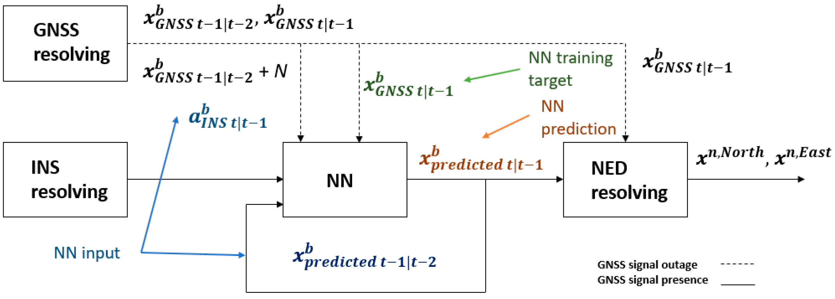
2.2. Neural Network Localisation Scheme Set-Up

We propose a displacement estimation model to minimise the effect of the noise in the accelerometer, as illustrated in Figure 1. The proposed model, which is analogous to the functioning of a closed-loop or feedback control system, operates in prediction mode by feeding back the output of the neural network at t 1 / t 2   and the vehicles’ acceleration at time window t / t 1 into the neural network in order to estimate the distance covered by the vehicle within the current window t / t 1 , as shown in Figure 2.
However, as presented in Figure 1, during the training phase, the NN is fed with the GNSS estimated displacement rather than the output of the NN. Both models (training and prediction) are structured this way due to the availability of the GNSS signal during the training phase and its absence in the prediction phase. The NN’s output is thus setup to mimic the functionality of the GNSS resolved displacement at window t 1 / t 2 during the prediction operation.
Howbeit, as the NN’s output never matches the GNSS displacement, the challenge becomes one of minimising the effect of the inexactness of the previous NN’s estimation on the performance of the prediction model. We set about to address this by introducing a controlled random white Gaussian noise N with a normal distribution N ~   N   ( μ ,   σ 2 ) to one of the inputs of the NN; the GNSS resolved displacement within the previous time window, during the training phase. Where the mean μ , and the and the variance σ 2 , are determined experimentally from a sample displacement resolving of the GNSS and INS signals. This approach attempts to aid the NN to account for the impreciseness in the prediction output. Figure 1 and Figure 2 shows the training and prediction set-up of the displacement model, respectively.
Furthermore, we adopt a much simpler approach towards the estimation of the vehicles orientation rate as we found no performance benefit in utilising the feedback approach presented in the previous paragraphs. On the orientation rate estimation, the NN is made to learn the relationship between the yaw rate as provided by the gyroscope and the ground truth (yaw rate) calculated from the information provided by the GNSS.

3. Data Collection, Experimental Setup and NN Model Selection

3.1. Dataset

The IO-VNBD dataset, consisting of 98 h of driving data collected over 5700 km of travel and characterised by diverse driving scenarios (publicly available at https://github.com/onyekpeu/IO-VNBD) was used in this study [24]. The dataset captures information such as the vehicle’s longitudinal acceleration, yaw rate, heading, GPS co-ordinates (latitude, longitude) at each time instance from the Electric Control Unit (ECU) of the vehicle with a sampling interval of 10 Hz. Details of the sensors used in our research can be found in Reference [24]. A Ford Fiesta Titanium was used for the data collection as shown in Figure 3. Table 1, Table 2 and Table 3 present the data subsets used in this study.

3.1.1. Performance Evaluation Metrics

The performance of both the INS- and NN-based approaches are evaluated using the metrics defined below:
Cumulative Root Squared Error (CRSE)—The CRSE measures the cumulative root squared of the prediction error every second for the total duration of the GNSS outage defined as 10 s. It ignores the contributions of the negative sign of the error estimations, enabling a better understanding of the performance of the positioning techniques.
CRSE =   t = 1 N t e p r e d 2
Cumulative Absolute Error (CAE)—The CAE measures the absolute error of the prediction every second and summates the values throughout the duration of the GNSS outage, contrastingly to the CRSE, signs are not ignored. This tool is useful to better understand if the position technique is generally under or over predicting points and how prediction variance affects the overall positioning of the vehicle after the 10 s outage period.
CAE =   t = 1 N t e p r e d .
Average Error Per Second (AEPS)—The AEPS measures the average error of the prediction every second of the GNSS outage. It is useful to compare the general performance of the models and has uses in showing any significant outliers.
A EPS =   1 N t   .   t = 1 N t e p r e d .
Mean ( μ )—The mean of the CRSE, CAE and AEPS across all test sequences within each scenario is evaluated to reveal the average performance of the positioning technique in each scenario.
μ C R S E =     1 N s i = 1 N s C R S E ,   μ C A E =     1 N s i = 1 N s C A E ,   μ A E P S =     1 N s i = 1 N s A E P S .
Standard Deviation ( σ )—The standard deviation measures the variation of the CRSEs, CAEs and AEPSs of the sequences of each test scenario.
σ C R S E = ( C R S E i μ ) 2 N s   ,   σ C A E = ( C R S E i μ ) 2 N s ,   σ A E P S = ( C R S E i μ ) 2 N s .
where N t is GNSS outage length of 10 s,   t is the sampling period, e p r e d is the prediction error and N s is the total number of test sequences in each scenario.
Minimum (min)—The minimum metric informs of the minimum CRSE, CAE and AEPS of all sequences evaluated in each test scenario.
Maximum (max)—The maximum CRSE, CAE and AEPS provide information of the maximum CRSE of all sequences evaluated in each test scenario. It provides information on the possible accuracy of the positioning techniques in such scenarios. It is our rational that the max metric holds more significance compared to the μ and min, as it captures the performance of the vehicle in each challenging scenario explored and further informs on the accuracy of the investigated techniques in each scenario.

3.1.2. Neural Network Comparative Analysis

The proliferation of Deep Learning and the internet of things on low memory devices, increasing sensing and computing applications and capabilities promise to transform the performance of such devices on complex sensing tasks. The key impediment to the wider adoption and deployment of neural network-based sensing application is their high computation cost. Therefore, there is the need to have a more compact parameterization of the neural network models. To this end, we evaluate the performance of the MLP, IDNN, vanilla RNN (vRNN), GRU and LSTM on the roundabout scenario across different parameterization for model efficiency.
From our study, we observe that the IDNN, vRNN and GRU achieves a max CRSE orientation rate of 0.34, followed by the LSTM recording a max C R S E of 0.35 rad/s, whilst the MLP provided the worst performance of them all with a max C R S E of 0.97 rad/s. In an almost similar fashion, the IDNN, vRNN, LSTM and GRU obtain a max CRSE displacement of 17.96 m, whilst the MLP obtains a max C R S E of 156.23 m. However, as the IDNN is characterised by a significantly lower number of parameters compared to the GRU, LSTM and vRNN whilst providing similar CRSE scores across all NN studied and weight connections explored, we adopt it for use in learning the sensor noise in the accelerometer and gyroscope in this study. Table 4 shows the number of parameters characterizing each NN across the various weights investigated; 8, 16, 32, 64, 96, 128, 192, 256 and 320.
Furthermore, we observe that the number of weighted parameters has little influence on the performance of the displacement and orientation rate estimation model. However, we notice that the number of time steps in the recurrent NN models (recurrent in both layer architecture and input structure such as the IDNN) significantly influences the accuracy of the model’s prediction in both the orientation and displacement estimation. The performance of the IDNN across several time steps ranging from 2–14 are presented in Table 5 and Table 6.

3.1.3. Training of the IDNN Model

The displacement and orientation model were trained using the Keras–Tensorflow platform on the data subsets presented in Table 1, characterised by 800 min of drive time over a total travel distance of 760 km. The models are trained using a mean absolute error loss function and an adamax optimiser. In the hidden layers, 10% of units were dropped from the hidden layers in the IDNN to avoid overfitting. Furthermore, to avoid learning bias, all the features that were fed to the neural network were standardised between 0 and 1. Table 7 highlights the parameters characterising the training of the neural network approaches investigated.

3.1.4. Testing of the IDNN Model

The data subsets used to investigate the performance of the INS and Neural Networks on the challenging scenarios are presented in Table 2 and Table 3. Although then evaluated on complex scenarios as previously mentioned, such as illustrated in Figure A1, Figure A2 and Figure A3 in Appendix A, the performance of the INS and NN modelling technique is first examined on the V-Vw12 dataset, which presents a relatively easier scenario; i.e., an approximate straight-line travel on the motorway. The evaluation of the latter scenario aims at gauging the performance of the technique in a relatively simpler driving situation. Nonetheless, the Motorway scenario could be challenging to track due to the huge distance covered per second. The evaluation is conducted on sequences of 10 s with a prediction frequency of 1 s. GPS outages are assumed on the test scenarios, for the purpose of the investigation.

4. Results and Discussion

The performance of the dead reckoned INS (INS DR) and proposed NN approaches are analysed comparatively across several GPS outage simulated sequences, each of 10 s length. The positioning techniques are first analysed on a less challenging scenario involving vehicle travel on an approximate straight line on the motorway. Further analysis is then done on more challenging scenarios such as hard brake, roundabouts, quick changes in acceleration and sharp cornering and successive left and right turns using the performance metrics defined in Section 3.1.

4.1. Motorway Scenario

In evaluating the performance of the INS and the NN approaches on vehicular motion tracking, both techniques are investigated on a less challenging trajectory characterised by an approximate straight-line drive on the motorway. The results, as shown on Table 8, show that across all 9 test sequences, the INS records its best and average displacement and orientation rate CRSE of 1.63 m, 15.01 m, and 0.08 rad/s, 0.13 rad/s, respectively. However, we observe that the NN outperforms the INS significantly on the displacement and orientation estimation across all metrics, as illustrated in Figure 4. Comparatively, the best and average displacement and orientation rate CRSE of the NN approach is recorded as 0.84 m and 1.93 m, and 0.08 rad/s and 0.13 rad/s. Essentially, this shows that the NN is able to offer up to an 89% improvement on the displacement max CRSE metric after about 268 m of travel. Achieving a CAE best of 0.16 m Northwards and 0.016 m Eastwards, the results also indicate that it is possible to estimate the vehicle position with lane-level accuracy using the proposed approach. Being the lowest errors across all scenarios evaluated as shown in Figure 4, Figure 5, Figure 6 and Figure 7, we can infer that this was the least challenging scenario due to minimal accelerations and directional change. Furthermore, the reliability of the NN in consistently tracking the vehicles’ motion with such accuracy is highlighted by its low standard deviation of 0.84. Figure 8b shows the trajectory of the vehicle along the motorway.

4.2. Roundabout Scenario

The roundabout scenario is one of the most challenging for both the vehicular displacement and orientation rate estimation. The difficulty encountered by the INS and NN in accurately tracking the vehicle’s motion is graphically shown in Figure 9 with a comparative illustration to other investigated scenarios presented in Figure 5, Figure 6 and Figure 7. The results so obtained as presented on Table 9 show that the NN recorded a lower displacement (maximum CRSE and CAE of 17.96 m and 16.80 m) than the INS (maximum CRSE and CAE displacement of 171.92 m) as well as a lower orientation rate (maximum CRSE and CAE of 0.38 rad/s and 0.05 rad/s, respectively) compared to the INS (maximum CRSE and CAE of 5.71 rad/s and 2.14 rad/s, respectively). The relatively lower standard deviation across all analysed metrics is evidence that the NN is able to more consistently track the vehicles position and orientation on the roundabout scenario but less consistently on other investigated scenarios. The roundabout scenario study was carried out across 11 test sequences over a maximum travel distance of approximately 197 m. Figure 8a shows a sample trajectory of the vehicle on the roundabout scenario analysis.

4.3. Quick Changes in Vehicles Acceleration Scenario

The results presented in Table 10 illustrate the performance of the NN-based approached over the INS in the quick changes in acceleration scenario. From observation, it can be seen that the neural network significantly outperforms the INS across all metrics employed, with a maximum CRSE of 8.62 m, 0.33 rad/s for the INS against 79.05 m and 0.67 rad/s for the INS over a maximum distance of approximately 220 m covered. This shows, as expected, that the INS and NN found it more challenging to estimate the displacement of the vehicle compared to the orientation rate. On other metrics, the NN obtains an average CAE, CRSE and AEPS of 5.30 m, 0.93 m and 0.05 m/s compared to that of the INS recorded as 38.92 m, 26.23 m and 0.43 m/s2 across all 13 test sequences evaluated offering up to a 92% improvement on the INS orientation rate estimation. Figure 10 graphically illustrates the evolution of the error across sample sequences on the CRSE and CAE metrics. A comparison of the performance of both approaches across all scenarios investigated is further presented in Figure 5, Figure 6 and Figure 7.

4.4. Hard Brake Scenario

The performance of the NN over the INS in the hard-brake scenario is evaluated over 17 test sequences averaging 188 m of travel with a 259 m maximum journey length. From Table 11, we observe that much to our expectations, the hard brake scenario proves to be more of a challenge for the accelerometer than the gyroscope as the INS struggles to accurately estimate the displacement and orientation rate of the vehicle within the simulated GPS outage period. As further emphasized on Figure 11 and Figure 5, Figure 6 and Figure 7, the NN significantly outperforms the INS DR across all performance metrics employed by max and average CRSE of 15.80 m, 0.25 rad/s and 6.82 m, 0.09 rad/s for the NN compared to 133.12 m, 1.89 rad/s and 41.07 m and 0.37 rad/s, respectively, of the INS DR. The reliability of the NN in consistently correcting the INSs estimations to such accuracy is further established by its σ value of 4.23 and 0.08.

4.5. Sharp Cornering and Successive Left–Right Turns Scenario

The sharp cornering and successive right–left turn scenario appears to be one of the most challenging for the INS on the CAE metric (see Figure 5, Figure 6 and Figure 7 and Figure 12). This scenario investigation involves analysis on 40 test sequences over a maximum travel distance of approximately 109 m. Reporting on the results presented in Table 12, it can be observed that the INS has a maximum CRSE and CAE displacement of 92.06 m compared to 12.71 m and 8.49 m, respectively, of the NN. On the orientation rate, the NN performs significantly better than the INS with a maximum CRSE and CAE of 0.41 rad/s and 0.13 rad/s against the INS’s performance of 4.29 rad/s and 3.47 rad/s. These results further highlight the capability of the NN to significantly improve vehicular localisation during GPS outages with its reliability assured by its relatively low standard division. An example trajectory of the vehicle during the sharp cornering and successive left and right turn is shown in Figure 13.

5. Conclusions

We propose a Neural Network-based approach inspired by the operation of the feedback control system to improve the localisation of autonomous vehicles and robots alike in challenging GPS deprived environments. The proposed approach is analytically compared to the INS specifically in scenarios characterised by hard braking, roundabouts, quick changes in vehicular acceleration, motorway, sharp cornering and successive left and right turns. By estimating the displacement and orientation rate of the vehicle within a GPS outage period, we showed that the Neural Network-based positioning approach outperforms the INS significantly in all investigated scenarios, by providing up to 89.55% improvement on the displacement estimation and 93.35% on the orientation rate estimation.
Nevertheless, we encountered the problem of poor model generalisation due to the varying characteristics of the sensor noise and bias in different journey domains as well as slight variations in the vehicular environment, trajectory and dynamics. These factors cause discrepancies between the training data and test data, hindering better estimations. There is, therefore, the need to create a model capable of accounting for the variations in the sensor’s characteristics and environments towards the end purpose of robustly and accurately tracking the motion of the vehicle in various terrains. This will be the subject of our future research.

Author Contributions

Conceptualization, U.O. and S.K.; methodology, U.O.; validation, U.O.; formal analysis, U.O.; resources, U.O. and S.K.; writing—original draft preparation, U.O.; writing—review and editing, S.K. and V.P.; visualization, U.O.; supervision, S.K. and V.P. All authors have read and agreed to the published version of the manuscript.

Funding

This research received no external funding.

Institutional Review Board Statement

Not applicable.

Informed Consent Statement

Not applicable.

Data Availability Statement

The dataset used in this study is available at https://github.com/onyekpeu/IO-VNBD and described in [24].

Conflicts of Interest

The authors declare no conflict of interest.

Appendix A

Figure A1. The variations in the (a) vehicle’s angular velocity in the roundabout scenario and (b) vehicle’s acceleration in the quick changes in acceleration scenario.
Applsci 11 01270 g0a1
Figure A2. The variations in the vehicle’s acceleration in the hard brake scenario.
Applsci 11 01270 g0a2
Figure A3. The variations in the vehicle’s angular velocity in the sharp cornering and successive left and right turn scenario.
Applsci 11 01270 g0a3

References

  1. Onyekpe, U.; Kanarachos, S.; Palade, V.; Christopoulos, S.G. Vehicular Localisation at High and Low Estimation Rates during GNSS Outages: A Deep Learning Approach. Deep Learning Applications, Volume 2. Advances in Intelligent Systems and Computing, Vol 1232; Arif Wani, V.P.M., Taghi, K., Eds.; Springer Singapore: Singapore, 2020; pp. 229–248. [Google Scholar]
  2. Teschler, L. Inertial Measurement Units will Keep Self-Driving Cars on Track. 2018. Available online: https://www.microcontrollertips.com/inertial-measurement-units-will-keep-self-driving-cars-on-track-faq/ (accessed on 5 June 2019).
  3. Santos, G.A.; Da Costa, J.P.C.L.; De Lima, D.V.; Zanatta, M.D.R.; Praciano, B.J.G.; Pinheiro, G.P.M.; De Mendonca, F.L.L.; De Sousa, R.T. Improved localization framework for autonomous vehicles via tensor and antenna array based GNSS receivers. In Proceedings of the 2020 Workshop on Communication Networks and Power Systems (WCNPS), Brasilia, Brazil, 12–13 November 2020; pp. 1–6. [Google Scholar] [CrossRef]
  4. Nawrat, A.; Jedrasiak, K.; Daniec, K.; Koteras, R. Inertial Navigation Systems and Its Practical Applications. In New Approach of Indoor and Outdoor Localization Systems; Elbakhar, F., Ed.; InTechOpen: London, UK, 2012. [Google Scholar]
  5. Chen, C.; Lu, X.; Markham, A.; Trigoni, N. IONet: Learning to Cure the Curse of Drift in Inertial Odometry. arXiv 2018, arXiv:1802.02209. [Google Scholar]
  6. Noureldin, A.; El-Shafie, A.; Bayoumi, M. GPS/INS integration utilizing dynamic neural networks for vehicular navigation. Inf. Fusion 2011, 12, 48–57. [Google Scholar] [CrossRef]
  7. Aftatah, M.; Lahrech, A.; Abounada, A.; Soulhi, A. GPS/INS/Odometer Data Fusion for Land Vehicle Localization in GPS Denied Environment. Mod. Appl. Sci. 2016, 11, 62. [Google Scholar] [CrossRef]
  8. Mikov, A.; Panyov, A.; Kosyanchuk, V.; Prikhodko, I. Sensor Fusion For Land Vehicle Localization Using Inertial MEMS and Odometry. In Proceedings of the 2019 IEEE International Symposium on Inertial Sensors and Systems (INERTIAL), Naples, FL, USA, 1–5 April 2019; pp. 1–2. [Google Scholar] [CrossRef]
  9. Malleswaran, M.; Vaidehi, V.; Jebarsi, M. Neural networks review for performance enhancement in GPS/INS integration. In Proceedings of the 2012 International Conference on Recent Trends in Information Technology, Chennai, India, 19–21 April 2012; pp. 34–39. [Google Scholar] [CrossRef]
  10. Malleswaran, M.; Vaidehi, V.; Mohankumar, M. A hybrid approach for GPS/INS integration using Kalman filter and IDNN. In Proceedings of the 2011 Third International Conference on Advanced Computing, Chennai, India, 14–16 December 2011; pp. 378–383. [Google Scholar] [CrossRef]
  11. Malleswaran, M.; Vaidehi, V.; Sivasankari, N. A novel approach to the integration of GPS and INS using recurrent neural networks with evolutionary optimization techniques. Aerosp. Sci. Technol. 2014, 32, 169–179. [Google Scholar] [CrossRef]
  12. Malleswaran, M.; Vaidehi, V.; Deborah, S.A. CNN based GPS/INS data integration using new dynamic learning algorithm. In Proceedings of the 2011 International Conference on Recent Trends in Information Technology (ICRTIT) 2011, Chennai, India, 3–5 June 2011; pp. 211–216. [Google Scholar] [CrossRef]
  13. Chen, C.; Lu, X.; Wahlstrom, J.; Markham, A.; Trigoni, N. Deep Neural Network Based Inertial Odometry Using Low-cost Inertial Measurement Units. IEEE Trans. Mob. Comput. 2019, 1. [Google Scholar] [CrossRef]
  14. Brossard, M.; Barrau, A.; Bonnabel, S. AI-IMU Dead-Reckoning. IEEE Trans. Intell. Veh. 2020, 5, 585–595. [Google Scholar] [CrossRef]
  15. Malleswaran, M.; Vaidehi, V.; Saravanaselvan, A.; Mohankumar, M. Performance analysis of various artificial intelligent neural networks for gps/ins integration. Appl. Artif. Intell. 2013, 27, 367–407. [Google Scholar] [CrossRef]
  16. Chiang, K.-W. The Utilization of Single Point Positioning and Multi-Layers Feed-Forward Network for INS/GPS Integration. Available online: https://www.ion.org/publications/abstract.cfm?articleID=5201 (accessed on 5 June 2019).
  17. Sharaf, R.; Noureldin, A.; Osman, A.; El-Sheimy, N. Online INS/GPS integration with a radial basis function neural network. IEEE Aerosp. Electron. Syst. Mag. 2005, 20, 8–14. [Google Scholar] [CrossRef]
  18. Dai, H.-F.; Bian, H.-W.; Wang, R.-Y.; Ma, H. An INS/GNSS integrated navigation in GNSS denied environment using recurrent neural network. Def. Technol. 2020, 16, 334–340. [Google Scholar] [CrossRef]
  19. Fang, W.; Jiang, J.; Lu, S.; Gong, Y.; Tao, Y.; Tang, Y.; Yan, P.; Luo, H.; Liu, J. A LSTM Algorithm Estimating Pseudo Measurements for Aiding INS during GNSS Signal Outages. Remote. Sens. 2020, 12, 256. [Google Scholar] [CrossRef] [Green Version]
  20. Simons-Morton, B.G.; Ouimet, M.C.; Wang, J.; Klauer, S.G.; Lee, S.E.; Dingus, T.A. Hard Braking Events Among Novice Teenage Drivers By Passenger Characteristics. In Proceedings of the International Driving Symposium on Human Factors in Driver Assessment, Training, and Vehicle Design, Santa Fe, NM, USA, 24–27 June 2009; Volume 2009, pp. 236–242. [Google Scholar] [CrossRef]
  21. Kok, M.; Hol, J.D.; Schön, T.B. Using Inertial Sensors for Position and Orientation Estimation. Found. Trends Signal Process. 2017, 11, 1–153. [Google Scholar] [CrossRef] [Green Version]
  22. VBOX Video HD2. Available online: https://www.vboxmotorsport.co.uk/index.php/en/products/video-loggers/vbox-video (accessed on 26 February 2020).
  23. Pietrzak, M. Vincenty · PyPI. Available online: https://pypi.org/project/vincenty/ (accessed on 12 April 2019).
  24. Onyekpe, U.; Palade, V.; Kanarachos, S.; Szkolnik, A. IO-VNBD: Inertial and Odometry Benchmark Dataset for Ground Vehicle Positioning. arXiv 2020, arXiv:2005.01701. [Google Scholar]
Figure 1. Training set-up of the proposed displacement estimation model.
Applsci 11 01270 g001
Figure 2. Prediction set-up of the proposed displacement estimation model.
Applsci 11 01270 g002
Figure 3. Data collection vehicle, showing sensor locations [2].
Applsci 11 01270 g003
Figure 4. Showing the evolution of the estimation error over time in the motorway scenario based on the (a) Displacement CRSE, (b) Displacement cumulative absolute error (CAE), (c) Orientation rate CRSE and (d) Orientation rate CAE.
Applsci 11 01270 g004
Figure 5. Showing the comparison of the CAE performance of the IDNN and INS DR across all investigated scenarios on the (a) displacement estimation and (b) orientation rate estimation.
Applsci 11 01270 g005
Figure 6. Showing the comparison of the average error per second (AEPS) performance of the IDNN and INS DR across all investigated scenarios on the (a) displacement estimation and (b) orientation rate estimation.
Applsci 11 01270 g006
Figure 7. Showing the comparison of the CRSE performance of the IDNN and INS DR across all investigated scenarios on the (a) displacement estimation and (b) orientation rate estimation.
Applsci 11 01270 g007
Figure 8. Sample trajectory of the (a) V-Vta11 roundabout data subset of the Inertia and Odometry Vehicle Navigation Dataset (IO-VNBD) and (b) V-Vw12 motorway data subset of the IOVNBD.
Applsci 11 01270 g008
Figure 9. Showing the evolution of the estimation error over time in the roundabout scenario based on the (a) Displacement CRSE, (b) Displacement CAE, (c) Orientation rate CRSE and (d) Orientation rate CAE.
Applsci 11 01270 g009
Figure 10. Showing the evolution of the estimation error over time in the quick changes in acceleration scenario based on the (a) Displacement CRSE, (b) Displacement CAE, (c) Orientation rate CRSE and (d) Orientation rate CAE.
Applsci 11 01270 g010
Figure 11. Showing the evolution of the estimation error over time in the hard brake scenario based on the (a) Displacement CRSE, (b) Displacement CAE, (c) Orientation rate CRSE and (d) Orientation rate CAE.
Applsci 11 01270 g011
Figure 12. Showing the evolution of the estimation error over time in the hard brake scenario based on the (a) Displacement CRSE, (b) Displacement CAE, (c) Orientation rate CRSE and (d) Orientation rate CAE.
Applsci 11 01270 g012
Figure 13. Trajectory of V-Vw8 sharp cornering and successive left and right turns data subset of the IO-VNBD.
Applsci 11 01270 g013
Table 1. Inertia and Odometry Vehicle Navigation (IO-VNB) data subsets used for the model training [24].
IO-VNB DatasetFeatures
V-Vta1aWet Road, Gravel Road, Country Road, Sloppy Roads, Round About (×3), Hard Brake on wet road, Tyre Pressure A
V-Vta2Round About (×2), A Road (A511, A5121, A444), Country Road, Hard Brake, Tyre Pressure A
V-Vta8Town Roads (Build-up), A-Roads (A511), Tyre Pressure A
V-Vta10Round About (×1), A—Road (A50), Tyre Pressure A
V-Vta16Round-About (×3), Hilly Road, Country Road, A-Road (A515), Tyre Pressure A
V-Vta17Hilly Road, Hard-Brake, Stationary (No Motion), Tyre Pressure A
V-Vta20Hilly Road, Approximate Straight-line travel, Tyre Pressure A
V-Vta21Hilly Road, Tyre Pressure A
V-Vta22Hilly Road, Hard Brake, Tyre Pressure A
V-Vta27Gravel Road, Several Hilly Road, Potholes, Country Road, A-Road (A515), Tyre Pressure A
V-Vta28Country Road, Hard Brake, Valley, A-Road (A515)
V-Vta29Hard Brake, Country Road, Hilly Road, Windy Road, Dirt Road, Wet Road, Reverse (×2), Bumps, Rain, B-Road (B5053), Country Road, U-Turn (×3), Windy Road, Valley, Tyre Pressure A
V-Vta30Rain, Wet Road, U-Turn (×2), A-Road (A53, A515), Inner Town Driving, B-Road (B5053), Tyre Pressure A
V-Vtb1Valley, rain, Wet-Road, Country Road, U-T urn (×2), Hard-Brake, Swift-Manoeuvre, A—Road (A6, A6020, A623, A515), B-Road (B6405), Round About (×3), day Time, Tyre Pressure A
V-Vtb2Country Road, Wet Road, Dirt Road, Tyre Pressure A
V-Vtb3 Reverse, Wet Road, Dirt Road, Gravel Road, Night-time, Tyre Pressure A
V-Vtb5Dirt Road, Country Road, Gravel Road, Hard Brake, Wet Road, B Road (B6405, B6012, B5056), Inner Town Driving, A-Road, Motorway (M42, M1), Rush hour(Traffic) Round-About (×6), A-Road (A5, A42, A38, A615, A6), Tyre Pressure A
V-Vw4Round-About (×77), Swift-Manoeuvres, Hard-Brake, Inner City Driving, Reverse, A-Road, Motorway (M5, M40, M42), Country Road, Successive Left-Right Turns, Daytime, U-Turn (×3), Tyre Pressure D
V-Vw5Successive Left-Right Turns, Daytime, Sharp Turn Left/Right, Tyre Pressure D
V-Vw14bMotorway (M42), Night-time, Tyre Pressure D
V-Vw14cMotorway (M42), Round About (×2), A-Road (A446), Night-time, Hard Brake, Tyre Pressure D
V-Vfa01A-Road (A444), Round About (×1), B–Road (B4116) Day Time, Hard Brake, Tyre Pressure A
V-Vfa02B-Road (B4116), Round About (×5), A Road (A42, A641), Motorway (M1, M62) High Rise Buildings, Hard Brake, Tyre Pressure C
V-Vfb01aCity Centre Driving, Round-About (×1), Wet Road, Ring Road, Night, Tyre Pressure C
V-Vfb01bMotorway (M606), Round-About (×1), City Roads Traffic, Wet Road, Changes in Acceleration in Short Periods of Time, Night, Tyre Pressure C
V-Vfb02bRound About (×1), Bumps, Successive Left Right Turns, Hard-Brake (×7), Zig-zag (×6), Night, Tyre Pressure D
Table 2. IO-VNB data test subset used in the less challenging scenario.
ScenarioIO-VNB Data SubsetTotal Time Driven, Distance Covered, Velocity and Acceleration
MotorwayV-Vw121.75 min, 2.64 km, 82.6–97.4 km/h, −0.06 to +0.07 g
Table 3. IO-VNB data test subset used in the challenging scenarios.
Challenging ScenariosIO-VNB Data SubsetTotal Time Driven, Distance Covered, Velocity and Acceleration
RoundaboutV-Vta111.0 min, 0.92 km, 26.8–97.7 km/h, −0.45 to +0.15 g
V-Vfb02d1.5 min, 0.84 km, 0.0–57.3 km/h, −0.33 to +0.31 g
Changes in accelerationV-Vfb02e1.6 min, 1.52 km, 37.4–73.9 km/h, −0.24 to +0.19 g
V-Vta121.0 min, 1.27 km, 44.7–85.3 km/h, 0.44 to +0.13 g
Hard BrakeV-Vw16b2.0 min, 1.99 km, 1.3–86.3 km/h, −0.75 to +0.29 g
V-Vw170.5 min, 0.54 km, 31.5–72.7 km/h, −0.8 to +0.19 g
V-Vta90.4 min, 0.43 km, 48.9–87.7 km/h, −0.6 to +0.14 g
Sharp Cornering and Successive left and right turns V-Vw62.1 min, 1.08 km, 3.3–40.7 km/h, −0.34 to +0.26 g
V-Vw72.8 min, 1.23 km, 0.4–42.2 km/h, −0.37 to +0.37 g
V-Vw82.7 min, 1.12 km, 0.0–46.4 km/h, −0.37 to +0.27 g
Table 4. Number of trainable parameters in each neural network (NN) across various weighted connections.
Number of Weighted Connections Number of Trainable Parameters
MLNN
(2-Layer)
vRNN
(2-Layer)
GRU
(2-Layer)
LSTM
(2-Layer)
IDNN
(2-Layer)
8336518524565
1697225657873161
3232183324653281449
6411533201953727051409
128435312,54537,50549,9854865
192960128,03383,905111,84110,369
25616,89749,665148,737198,27317,921
32026,24177,441232,001309,28127,521
Table 5. The performance evaluation based on the Cumulative Root Squared Error (CRSE) metric of the Input Delay Neural Network (IDNN) in each investigated scenario across several time steps on the orientation rate estimation.
Number of Time StepsMotorway (Rad/s)Roundabout (Rad/s)Quick Changes in Vehicle Acceleration (Rad/s)Hard Brake (Rad/s)Sharp Cornering (Rad/s)
20.050.410.380.280.52
30.060.620.330.330.56
40.060.590.340.350.51
50.060.600.380.340.41
60.050.610.390.350.43
70.050.630.370.320.47
80.050.600.370.320.46
90.050.600.350.340.45
100.060.610.350.280.51
110.060.580.360.250.50
120.050.380.380.280.51
130.060.620.330.320.51
140.060.590.340.350.49
Table 6. Showing the performance evaluation based on the CRSE metric of the IDNN in each investigated scenario across several time steps on the displacement estimation.
NNNumber of Time StepsMotorway (m)Roundabout (m)Quick Changes in Vehicle Acceleration (m)Hard Brake (m)Sharp Cornering (m)
IDNN2651.41702.17571.99648.57425.56
4616.60655.22546.76580.01373.03
6610.61599.22524.41577.19346.92
8592.27595.09474.55557.50292.78
103.6017.968.7115.8014.55
123.2319.528.6219.3614.43
143.6320.539.5820.4512.71
vRNN217.1155.5833.3064.0942.64
47.8747.9222.4551.8125.95
67.2829.1016.5625.2822.58
83.8321.0810.2716.3914.02
103.6017.968.7115.8014.55
123.2319.528.6219.3614.43
143.6320.539.5820.4512.71
GRU221.1951.5436.6662.0445.82
425.0142.6230.1145.0526.19
620.2433.7224.6423.8722.20
811.3324.1415.1617.5915.47
103.6017.968.7115.8014.55
123.2319.528.6219.3614.43
143.6320.539.5820.4512.71
LSTM232.9754.2134.7460.7837.53
418.2041.6226.7351.9428.21
66.1933.8216.4834.6820.39
84.1221.7511.4916.1813.8227
103.6017.968.7115.8014.55
123.2319.528.6219.3614.43
143.6320.539.5820.4512.71
Table 7. Training parameters for the IDNN.
ParametersDisplacement EstimationOrientation Estimation
Learning rate0.0040.001
Dropout10%10%
Sequence LengthSee Table 3See Table 2
Hidden layers22
Hidden neurons32 per layer32 per layer
Batch Size256256
Epochs4060
Table 8. Showing the performance of the IDNN and dead reckoned Inertial Navigation Systems (INS DR) on the motorway scenario.
IDNN (m)INS DR (m)IDNN (Rad/s)INS DR (Rad/s)
CRSE max3.2330.110.050.21
min0.841.630.020.08
μ1.9315.010.040.13
σ0.849.120.010.03
CAE max2.5630.110.020.13
min0.190.040.000.04
μ0.9613.330.010.10
σ0.8410.170.010.03
AEPS (/s)max0.060.300.000.00
min0.000.010.000.00
μ0.020.150.000.00
σ0.020.100.000.00
Total Distance Covered by vehiclemax268.40
min234.47
μ251.29
Number of Sequences evaluated9
Table 9. Showing the performance of the IDNN and INS DR on the roundabout scenario.
IDNN (m)INS DR (m)IDNN (Rad/s)INS DR (Rad/s)
CRSEmax17.96 171.92 0.385.71
min2.3619.420.020.17
μ8.6378.320.171.48
σ5.5152.330.131.77
CAE max16.80171.920.052.14
min0.519.420.000.03
μ5.47−57.600.010.62
σ5.3554.200.020.76
AEPS (/s)max0.341.760.010.08
min0.000.230.000.00
μ0.100.890.000.02
σ0.100.490.000.03
Total Distance Covered by vehicle max196.71
min19.89
μ104.93
Number of Sequences evaluated11
Table 10. Showing the performance of the IDNN and INS DR on the quick changes in acceleration scenario.
IDNN (m)INS DR (m)IDNN (Rad/s)INS DR (Rad/s)
CRSEmax8.6279.050.330.67
min2.3717.720.030.15
μ5.3038.920.160.28
σ2.1916.720.100.13
CAEmax3.9579.050.050.65
min2.3717.720.000.00
μ0.9326.230.020.18
σ2.8332.440.010.17
AEPS (/s)max0.150.910.010.02
min0.010.020.000.00
μ0.050.430.000.00
σ0.030.250.000.00
Total Distance Covered max220.08
min137.72
μ168.62
Number of Sequences evaluated13
Table 11. Showing the performance of the IDNN and INS DR on the hard brake scenario.
IDNN (m)INS DR (m)IDNN (Rad/s)INS DR (Rad/s)
CRSE max15.80133.120.251.89
min1.155.740.030.06
μ6.8241.070.090.37
σ4.2333.750.080.48
CAE max14.75133.120.051.17
min0.081.370.000.01
μ0.4426.500.020.21
σ3.8934.700.010.33
AEPS (/s)max0.211.970.000.01
min0.010.010.000.00
μ0.060.470.000.00
σ0.060.430.000.00
Total Distance Covered max258.79
min73.39
μ188.48
Number of Sequences evaluated17
Table 12. Showing the performance of the IDNN and INS DR on the sharp cornering and successive left and right turns scenario.
IDNN (m)INS DR (m)IDNN (Rad/s)INS DR (Rad/s)
CRSE max12.7192.060.414.29
min1.435.200.060.19
μ6.7739.350.191.99
σ2.8326.910.091.42
CAE max8.4992.060.133.47
min0.102.020.000.01
μ0.0111.34−0.01−0.07
σ2.2928.840.042.03
AEPS (/s)max0.250.940.020.16
min0.000.000.000.00
μ0.060.380.000.02
σ0.070.300.000.04
Total Distance Covered max109
min21
μ75
Number of Sequences evaluated40
Publisher’s Note: MDPI stays neutral with regard to jurisdictional claims in published maps and institutional affiliations.

