Featured Application
This work uses AFRBF-SMC to achieve the vehicle stability control after the estimation of the sideslip angle by ADUKF.
Abstract
This study is targeted at the key state parameters of vehicle stability controllers, the controlled vehicle model, and the nonlinearity and uncertainty of external disturbance. An adaptive double-layer unscented Kalman filter (ADUKF) is used to compute the sideslip angle, and a vehicle stability control algorithm adaptive fuzzy radial basis function neural network sliding mode control (AFRBF-SMC) is proposed. Since the sideslip angle cannot be directly determined, a 7-degrees-of-freedom (DOF) nonlinear vehicle dynamic model is established and combined with ADUKF to estimate the sideslip angle. After that, a vehicle stability sliding mode controller is designed and used to trace the ideal values of the vehicle stability parameters. To handle the severe system vibration due to the large robustness coefficient in the sliding mode controller, we use a fuzzy radial basis function neural network (FRBFNN) algorithm to approximate the uncertain disturbance of the system. Then the adaptive rate of the system is solved using the Lyapunov algorithm, and the systemic stability and convergence of this algorithm are validated. Finally, the controlling algorithm is verified through joint simulation on MATLAB/Simulink-Carsim. ADUKF can estimate the sideslip angle with high precision. The AFRBF-SMC vehicle stability controller performs well with high precision and low vibration and can ensure the driving stability of vehicles.
1. Introduction
With the intellectualizing of vehicles, the active safety control system becomes particularly important in ensuring human-vehicle safety. As an important component of this system, the vehicle stability controller can effectively prevent vehicles from sharp steering, sideslip, and overturn when additional yaw moment is needed (e.g., Active steering, anti-collision upon emergency, path planning, tracking control), and thus is critical in guaranteeing human-vehicle safety [1,2,3,4,5]. Despite the many studies on vehicle stability control, modeling of the vehicle, which is a highly nonlinear system, cannot accurately or quantitatively describe the disturbance caused by parameter perturbation, external environment, and other factors during real-world driving. The sideslip angle, a key parameter of vehicle stability control, cannot be directly determined by sensors given the consideration of costs and thus, is estimated by building observers based on multi-information fusion [6,7,8,9,10]. If a vehicle model cannot well reflect the real vehicle status or if the measured sideslip angle is largely different from the real value, the vehicle stability control quality will be lowered and vehicle instability cannot be effectively avoided.
Determination of the sideslip angle is the basis to develop stability control algorithms. In this field, Kalman filtering and its suboptimal filtering algorithms can well estimate the status of nonlinear systems and thus are widely applied [11]. When the model errors caused by inaccurate estimation of road surface friction are compensated by using sideslip angle speed feedback, the sideslip angle can be computed by combining the variable-structure extended Kalman filtering [12]. Based on the status constraints during estimation, the constrained unscented Kalman filtering was used to determine the sideslip angle by considering the measured noise and nonlinearity of the system [13]. An unscented Kalman filter based on the ANFIS observer was proposed and used to introduce the measurable parameters of the vehicle sensor into the unscented Kalman filter, which thereby computed the sideslip angle [14]. A body sideslip angle adaptive dynamic calibrated variable structure observer based on unscented Kalman filtering was proposed and used to compensate the model uncertainty by using the parameter adaptive unscented Kalman observer. Then the variable structure observer was used to compensate the errors in the strongly nonlinear zone, and thereby the sideslip angle was determined [15]. Based on the Rational tire model, the tire characteristics under different driving conditions were described by online estimation and updating tire parameters, and the sideslip angle was estimated using the extended Kalman filtering algorithm [16]. A novel sideslip angle algorithm integrating deep neural network and nonlinear Kalman filtering was proposed and used to estimate sideslip angle [17]. The above algorithms based on Kalman filtering and its suboptimal filtering algorithms can be well used to estimate the vehicle sideslip angle, but the unscented Kalman filtering algorithms are limited by the low effectiveness for highly nonlinear systems. Moreover, extended Kalman filtering needs to calculate estimating the Jacobian matrix, which is very complex computationally. The adaptive double-layer unscented Kalman filter (ADUKF), because of high filtering precision, is applicable to the status estimation of highly nonlinear systems [18], and thus was selected here to compute vehicle sideslip angle.
During the design and development of vehicle stability control algorithms, it is needed to build a dynamic model which can reflect the real vehicles. However, the existing vehicle models cannot accurately represent real vehicles, owing to parameter perturbation, environmental complexity and variability, simplification of modeling, and other factors. The sliding mode controller (SMC), because of its high robustness and finite time convergence, can converge in uncertain disturbance systems and has been applied into practical engineering [19,20,21]. However, in the case of severe system disturbance, a large robustness coefficient should be selected during the design of smcs, but this will cause serious vibration. To solve this problem, researchers have changed the criterion of robustness coefficient selection from uncertainty disturbance to the approximation error of system disturbance, which will reduce the robustness coefficient and system vibration. Recently, the uncertainty disturbance during practical engineering modeling has been extensively studied. The uncertainty of tire rigidity upon vehicle steering can be described by the norm constraint [22]. The nonlinear disturbance of systems was handled by combining the robust integration of an error controller with the adaptive controller [23]. During wheel slip tracking control, a radial basis function neural network (RBFNN) was used as an uncertainty observer to estimate the uncertainty during modeling [24]. A linear uncertainty vehicle model with steering rigidity uncertainty was built [25]. A function recursive fuzzy neural network uncertainty estimator [26] and a self-organizing function-link fuzzy cerebellar model articulation controller [27] were used to approximate the unknown nonlinear terms of vehicle dynamics during ABS control. Nonlinear adaptive backstepping control algorithms based on model parameter adaptive controller with slide mode observer [28] and on dynamic recursive radial basis function network uncertainty observer [29] were designed and used to observe the nonlinear uncertainty of permanent magnet direct-current generators. The above studies about uncertainty approximation are focused on a certain aspect of uncertainty, and the algorithms still should be improved further. As for systemic uncertainty, it can be approximated in both fuzzy systems and RBFNN systems. The advantage of fuzzy systems lies in the strong ability of fuzzy language utilization, which endows fuzzy systems with high inferring ability. In comparison, RBFNN systems possess strong generalization ability and simple network structures and can avoid unnecessary or redundant computation. By integrating the strong inferring ability of fuzzy systems and the strong learning ability of rbfnns, we proposed a fuzzy radial basis function neural network (FRBFNN) for uncertainty approximation.
The vehicle stability control algorithm proposed in this study is structurally illustrated in Figure 1. Firstly, a 7-degrees-of-freedom (DOF) nonlinear dynamic vehicle model based on the unitire model was built. Based on the parameters directly monitored by vehicle sensors and the 7-DOF model, we designed an ADUKF algorithm and used it to estimate the sideslip angle. Secondly, based on a 2-DOF linear vehicle reference model, the ideal values of the stability control parameters were outputted. Given the uncertainty of system modeling, we adopted a 2-DOF nonlinear vehicle model involving system uncertainty and additional yaw moment, and established an adaptive fuzzy radial basis function neural network sliding mode control (AFRBF-SMC), which was used to trace and control the ideal values of the control parameters. After the additional yaw moment was calculated by the controller, the braking torque was allocated according to the judgement of vehicle status, and the wheel cylinder pressure was outputted via the execution layer to the vehicle model. Thereby, closed-loop control of the vehicle stability system was accomplished.
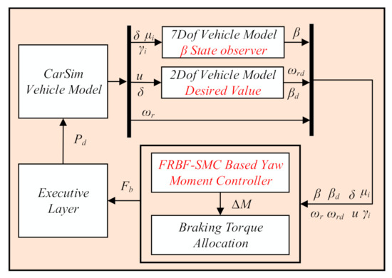
Figure 1.
The overall structure of the vehicle dynamics stability controller.
2. Estimation of Sideslip Angle
During the vehicle stability control, the sideslip angle is a key control parameter, and its estimation accuracy can directly affect the controlling quality. So far, the sideslip angle is mostly determined by estimation. For accurate estimation of this angle, we established a 7-DOF nonlinear vehicle dynamic model involving tire force, which was computed using the unitire model.
2.1. The 7-DOF Nonlinear Vehicle Dynamic Model
To fully reflect the state information of a driving vehicle, we built a 7-DOF nonlinear vehicle dynamic model involving the vehicle longitudinal movement, lateral movement, and yawing in the tire model (Figure 2). It is supposed that the center-of-mass of the vehicle is superposed with the origin of its driving coordinates, and the action of the steering system is ignored. Let the direction of its longitudinal motion be X-axis, the forward direction be positive; let the Y-axis pass the center-of-mass, the leftward direction be positive; let the torque and rolling angle on the horizontal plane pointing to the anticlockwise direction as positive.
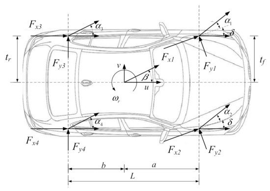
Figure 2.
Seven-degrees-of-freedom vehicle dynamic model.
The longitudinal movement, lateral movement and yawing of the vehicle are shown below.
The accelerations in the body coordinate system are converted to the accelerations and sideslip angle in the inertia coordinate system:
The sideslip angles and vertical loads of the four tires are shown below:
where is the entire vertical mass; is the distance from the center-of-mass to the front axle; is the distance from the center-of-mass to the rear axle; is the between-axle distance; and are half of the front-wheel distance and the rear wheel distance; is the above-ground height of the center-of-mass; and are the longitudinal and lateral velocity; and are the longitudinal and lateral accelerations in the inertia coordinate system; is the rotary inertia around the z-axis; is the yaw rate; is the front-wheel steering angle; is the sideslip angle; and are the longitudinal and lateral forces of tires; is the sideslip angle of tires; is the vertical loading of tires (where , 1, 2, 3, and 4 represent the left front wheel; right front wheel, left rear wheel, and right rear wheel respectively).
2.2. The Unitire Model
During practical driving, owing to the time-variable road conditions and driving environment, the tires are under an unstable status, which complicates the modeling of tires. Thus, building a tire model that can accurately describe the real movements of tires is the basis for research on vehicle dynamics. The unitire model featured by high modeling precision, excellent theoretical boundaries, and whole working condition coverage [30,31] was selected here and used to compute tire forces.
The longitudinal slip rate and lateral slip rate of the tire model are:
where is the longitudinal velocity at the center of a tire; is the lateral velocity at the center of the tire; is the valid rolling radius of the tire; is its rotating speed.
The relative longitudinal slip rate , relative lateral slip rate , and relative total slip rate of a tire are:
where is the vertical loading of a tire; and are the longitudinal friction factor and lateral friction factor; and are the longitudinal rigidity and lateral rigidity.
The longitudinal force , lateral force , and aligning torque of the tire are:
where and are the dimensionless longitudinal force and lateral force; is the longitudinal curvature factor or lateral curvature factor; is the aligning force arm;, , , and are the structural parameters of . The main parameters of the Unitire model are listed in Appendix A.
2.3. Design of Sideslip Angle Algorithm
The ADUKF algorithm was used to estimate the vehicle status parameters. This algorithm consists of an upper-layer UKF and a lower-layer UKF. ADUKF samples twice at time (k-1), including primary sampling and secondary sampling. Firstly, with an appropriate sampling strategy, N primary sampling points are selected, and then M secondary sampling points from each primary sampling point are chosen. The secondary sampling is a re-sampling of the results from the primary sampling. In the lower-layer UKF, the secondary sampling points with weights are predicted and updated. After that, the weights of the primary sampling points are updated. The updated secondary sampling points are weighted by the weights of the updated primary sampling points. The weighted status is considered as a prior status of the upper-layer UKF, and the primary sampling points are predicted and updated. Thereby, the whole ADUKF is finished.
According to the 7-DOF nonlinear vehicle dynamic model, we select:
- System status vector: ;
- Measuring status vector: ;
- Control input: ,
where is a wheel tire; is the road surface adhesion coefficient where the four tires are, where .
According to Equations (1)–(4), the state equation and observation equation of the vehicle system can be set up:
where is the nonlinear state equation; is the nonlinear observation equation; and are the status noise and observation noise with Gaussian white noise and are mutually independent from the status vector, and their covariance matrices are Q and R.
The system initial status is the initial value , and the initial covariance is . Owing to the presence of noise, the initial status should be dimension-expanded:
The specific steps for ADUKF are as follows:
(1) Initialize.
(2) Select Sigma sampling points by using the symmetrical sampling strategy and calculate corresponding weights.
Weights of sampling points are:
where is the number of sampling points; n is the number of status vector dimensions; is the status vector variance; is the ratio parameter used to lower the total prediction error.
(3) Update the lower-layer UKF.
At time , N sampling points are chosen by symmetrical sampling, and the sum of their weights and are determined. From each primary sampling point, M secondary sampling points are selected by using the same strategy, and the sum of their weights and is determined, where .
① update time:
② update measurement:
③ calculate covariance matrix:
④ compute lower-layer Kalman gain:
⑤ update status estimated values and covariance matrix:
(4) update upper-layer UKF.
① update weights:
where p is the importance density function; q is the suggested distribution function.
The updated weights are normalized:
② compute the initial value and covariance at time k:
③ update measurement:
Based on the prediction status and prediction covariance matrix at time k determined from the above equation, N weighted sampling points x are selected by using symmetrical sampling and their measurements are updated again:
④ calculate covariance matrix:
⑤ compute upper-layer Kalman gain:
⑥ update status estimated values and covariance matrix:
Through the above repetitions, the estimated value of the system at any time can be computed. The convergence of ADUKF is guaranteed by adjusting Q and R.
3. Design of Vehicle Stability Controller
After the estimation of sideslip angle, it was compared with the ideal value of controlled variables outputted from the 2-DOF linear reference model, which showed whether or not the vehicle needed intervention of stability control. Given the time variability of external disturbance and parameter input during real-world driving, the 2-DOF nonlinear vehicle dynamic model involving an uncertainty term and additional yaw moment is introduced to deduce the additional yaw moment controlling rate. Moreover, a FRBFNN system was adopted to estimate the uncertainty, which will lower the system shaking during the controlling process.
3.1. Two-DOF Linear Reference Model
The 2-DOF reference model is illustrated in Figure 3.
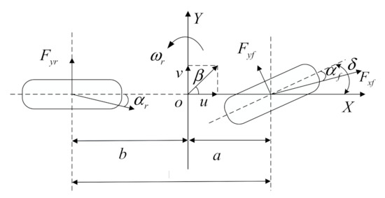
Figure 3.
Two-degrees-of-freedom vehicle dynamic model.
Where Fyf is the lateral force of the front wheel; Fyr is the lateral force of the rear wheel; v is the lateral velocity of the vehicle; u is the longitudinal velocity of the vehicle; is the sideslip angle of the front wheel; is the sideslip angle of the rear wheel; a is the distance from the front axle to the vehicle center-of-mass; b is the distance from the rear axle to the center-of-mass; is the steering angle of the front wheel; is the sideslip angle of center-of-mass; Is the yaw rate of the vehicle.
The dynamics equation of the 2-DOF model (Figure 3) is deduced as follows:
where Cf is the equivalent lateral stiffness of front axle tires; Cr is the equivalent lateral stiffness of rear axle tires; m is the whole vehicle mass; Iz is the rotary inertia of the vehicle around z-axis. The selection of tire lateral stiffness is based on the tire lateral characteristics. When the tire sideslip angle is small, the lateral force and the cornering angle are linear. It is considered that the ratio of cornering force and cornering angle is the lateral stiffness of vehicle tire under linear condition.
Figure 3 shows the dynamics model when the 2-DOF linear reference model is the ideal condition. The real vehicle is a highly nonlinear body under machine-electricity-liquid coupling. During vehicle modeling, the uncertainty caused by model simplification during the driving process and the disturbance induced by variation in the external environment both will affect the design and development of control algorithms. For this reason, disturbance is integrated as a nonlinear uncertainty term. Thus, the 2-DOF model involving a nonlinear uncertainty term and additional yaw moment is shown below:
where D1 is the integrated nonlinear disturbance term from lateral movement; D2 is the integrated nonlinear disturbance term from yawing; is the additional yaw moment; D1 and D2 are both bounded.
3.2. Expected Values of Control Variables
During the steady-state driving, , and , and from Equation (1), it is known that the yaw rate of the vehicle under ideal movement status is:
where is the desired yaw rate; L is the axel distance, ; K is the stability factor.
During real-world driving, the road surface adhesion coefficient will affect the driving status, so the maximum lateral acceleration should meet , where is the maximum lateral acceleration; is the road surface adhesion coefficient; g is the gravitational acceleration. The lateral acceleration can be expressed as:
By combining Equations (27) and (28), it is known that:
By combining Equations (27) and (29), the expected yaw rate is calibrated as follows:
During practical vehicle control, drivers hope that the sideslip angle is minimally small and can be maintained within a small range. For computational simplification, we define the expected value of sideslip angle as 0: .
3.3. Design of RBFNN-SMC Controller
As for synchronous control of yaw rate and sideslip angle, we design an SMC:
where is the weight coefficient of joint control of yaw rate and sideslip angle. During the convergence of the control system, the sliding mode function should meet: when , , namely: , , which ensures the convergence of the system.
Derivation of Equation (31) yields:
Substituting it into Equation (26), we have:
For simplification of computation, Equation (33) is rewritten as:
where:
In the above equation, since D1 and D2 are both bounded, then is bounded, or namely , then .
The SMC law of additional yaw moment is designed:
where , is the equivalent term; , is the robust term, .
By substituting Equation (36) to Equation (34), then:
Namely:
Since is the uncertainty disturbance, its value is affected by multiple factors. When is large, the robustness coefficient of the controller is also large, which will lead to severe vibration. Hence, to ensure the system vibration is small, we adopt an approximation function to approximate the nonlinear disturbance .
As for a nonlinear approximation problem, we combine the merits of RBFNN and fuzzy systems, and integrate them to approximate the nonlinear uncertainty .
The structure of a FRBFNN is shown in Figure 4, which consists of an input layer, a fuzzification layer, a fuzzy reasoning layer, and an output layer. After the input components are entered into the input layer, they are transferred to the fuzzification layer, and after connection with the fuzzy reasoning layer, the fuzzy rule matching is finished before fuzzy computation. Finally, the nodes in the output layer are weighed and outputted.
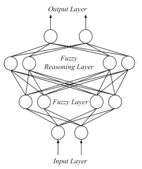
Figure 4.
Fuzzy radial basis function neural network structure diagram.
The first layer: the input layer.
The input and output of each node in this layer can be expressed as:
The second layer: the fuzzification layer.
Each node of this layer has a membership function, which is a Gaussian basis function. For the j-th node:
where is the central vector value of the j-th neuron in the hidden layer; is the Gaussian basis function width of neuron j in the hidden layer.
The third layer: the fuzzy reasoning layer.
This layer is connected to the fuzzification layer, so the fuzzy-rule matching and between-node fuzzy operation are realized. The output from each node j is the product of the inputted signals of this node:
where , is the number of i-th membership functions in the input layer, and the number of nodes in the fuzzification layer.
The fourth layer: the output layer.
The output in each node of this layer is the weighted sum of the inputted signals:
where l is the number of nodes in the output layer; is the connection matrix between the output nodes and the third-layer nodes.
The structure of the FRBFNN is 2-25-25-1 (input layer- fuzzification layer- fuzzy reasoning layer- fuzzy reasoning layer). Let the input be . Let , then and are the network output value and the actual value respectively, so the approximation error of the network is:
The adjustable parameters are calibrated using the gradient descent method. The target function is defined as:
The learning algorithm of the FRBFNN is:
Adjust the weights of the output layer:
The learning algorithm of the output layer is:
where is the learning rate, , and is the momentum factor, .
The membership function parameters of the input layer are adjusted as follows:
where:
The learning process of membership function parameters is:
From the above equation, the output of the FRBFNN system is:
where is the ideal network weight.
Then:
where .
In all, the additional yaw moment sliding mode control rate based on the FRBFNN is:
Substituting the above equation into Equation (34), we have:
With the above controller, the Lyapunov stability of the system is proved, and then a Lyapunov function is set up:
where . By deriving the Lyapunov function, we have:
Based on the Lyapunov stability, for the above equation, let , and the adaptive rules be , then:
The system satisfies the Lyapunov stability.
In all, when the system is under the AFRBF-SMC, the condition that the system meets Lyapunov stability is . The approximation error of the FRBFNN nonlinear estimator is far smaller than the upper boundary d of the disturbance term. Compared with SMC, the controller with additional yaw moment and based on AFRBF-SMC only needs a very small positive number . While the system meets convergence, it decreases slip mode vibration.
3.4. Allocation of Extra Yaw Moment
As for the additional yaw moment outputted from the controller, the rule of single-wheel braking force allocation is adopted, and it is allocated in the form of longitudinal braking force into the corresponding wheel, which is utilized in differential braking. The driver’s intention of steering is identified according to the steering wheel rolling angle and yaw rate. Together with the steering characteristics, the braking wheel is selected. The concrete selection of braking wheels is listed in Appendix B.
After the allocation of additional yaw moment, the target additional yaw moment is computed by the execution layer, so the target braking pressure needed by the braking wheel is determined. A hydraulic pressure braking is adopted in the actuator. The pressure control of the execution layer is not elaborated here.
4. Simulated Results and Analysis
MSC Carsim is a vehicle dynamics simulation software that can most accurately and effectively simulate the entire car kinetics. In this section, MATLAB/Simulink and MSC Carsim are combined for simulation to validate the new control algorithm. In MATLAB/Simulink, AFRBF-SMC vehicle stability controller is established. The initial weight of the FRBFNN is a random number within [−1, 1], the central vector cij is [−2 −1 0 1 2; −5 −2 0 2 5], and the Gaussian basis function width bj is 5. An entire vehicle model is built on MSC Carsim. The control effect of the controller is validated by using the front-wheel sine steering condition and double lane change (DLC). During the simulation, MSC Carsim inputs the real-time state parameters of the vehicle into the controller built by Simulink, and calculates the output control rate through the controller to the MSC Carsim vehicle model to realize the closed-loop control of the system. During the simulation, the simulation step taken as 0.001 s. The main parameters of the vehicle and the controller are listed in Appendix C.
4.1. Sinusoidal Steering Condition
On carsim, the road surface adhesion coefficient is set as 0.6, the initial vehicle speed is 108 km/h, the simulation time is 10 s, the steering wheel rolling angle is 0.25 Hz, and the amplitude 1 rad means sinusoidal driving. The steering wheel input is shown in Figure 5. The simulation results are shown in Figure 6a–j.
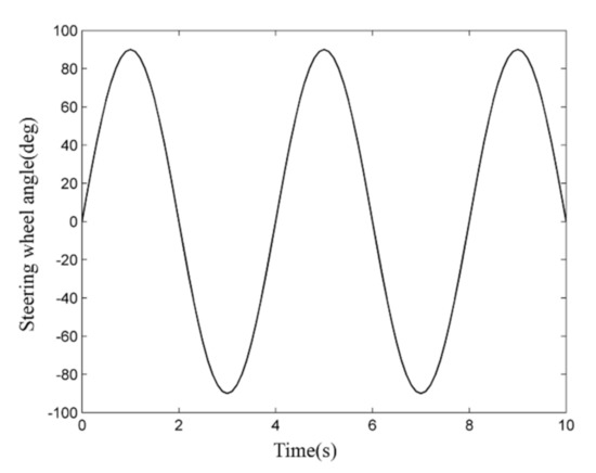
Figure 5.
The front wheel steering angle input.
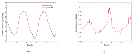
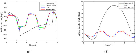
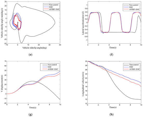
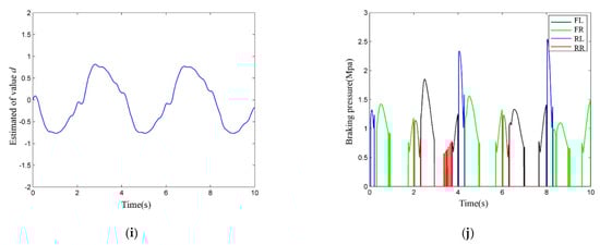
Figure 6.
The simulation results of the front wheel sinusoidal steering test: (a) the comparison of estimated sideslip angle and real value; (b) the sideslip angle estimation error; (c)the vehicle yaw rates; (d) the vehicle sideslip angle; (e) the phase plane of the vehicle sideslip angle and the vehicle sideslip angle rate; (f) the vehicle lateral acceleration; (g) the vehicle lateral displacement; (h) the vehicle longitudinal velocity; (i)the estimated of value d; (j) brake pressure of the braking wheels by adaptive fuzzy radial basis function neural network sliding mode control (AFRBF-SMC) controller.
The ADUKF can well estimate the sideslip angle with low errors and can meet the demand for vehicle stability control (Figure 6a,b). When the vehicle is under control without controller intervention, the yaw rate and sideslip angle both severely fluctuate, and after about 2.7 s, the expected value cannot be traced, so the vehicle enters an unstable status (Figure 6c–e). With the intervention by AFRBF-SMC and by SMC, both controllers can effectively ensure the stability of the target vehicle. The AFRBF-SMC can better trace the ideal value and causes less fluctuation compared with SMC, and the yaw rate and sideslip angle are closer to the ideal values. AFRBF-SMC, compared with SMC and the control-less status, makes the vehicle have better dynamics performance (Figure 6e–j). Clearly, with AFRBF-SMC, the certainty term and the cylinder pressure both change (Figure 6i,j). This is because when AFRBF-SMC is used to estimate the disturbance term, the vibration control effect is better than SMC, and the control rate of additional yaw moment is finer. Nevertheless, AFRBF-SMC causes more longitudinal dynamics interventions. As for lateral dynamics, AFRBF-SMC can ensure smaller lateral displacement and lower-fluctuation lateral acceleration. During sinusoidal steering, the overall performance of AFRBF-SMC is better.
4.2. Double Lane Change (DLC) Condition
The DLC test is used here [32]. The testing paths are set in Carsim. The road surface adhesion coefficient is 0.4, initial vehicle speed is 80 km/h, and simulation time is 10 s (Figure 7). The simulation results are shown in Figure 8a–j.
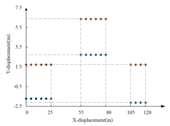
Figure 7.
The double lane change (DLC) test Lane layout.
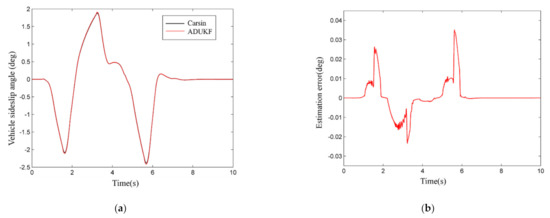
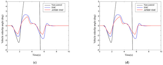
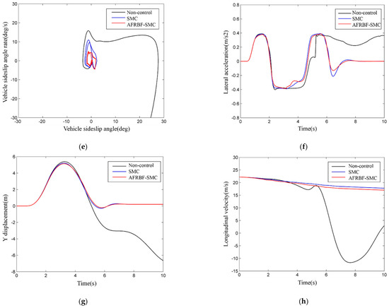
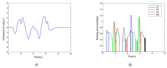
Figure 8.
The simulation results of the front wheel sinusoidal steering test: (a) the comparison of estimated sideslip angle and real value; (b) the sideslip angle estimation error; (c) the vehicle yaw rates; (d) the vehicle sideslip angle; (e) the phase plane of the vehicle sideslip angle and the vehicle sideslip angle rate; (f) the vehicle lateral acceleration; (g) the vehicle lateral displacement; (h) the vehicle longitudinal velocity; (i) the estimated of value d; (j) brake pressure of the braking wheels by AFRBF-SMC controller.
The ADUKF can well estimate the vehicle sideslip angle with low errors and can meet the demand for vehicle stability control (Figure 8a,b). With the absence of controller intervention, the yaw rate and sideslip angle both severely fluctuate, and after about 4.9 s, the yaw rate quickly increases and diverges, but the sideslip angle rapidly rises and diverges after about 2.3 s (Figure 8c–d). With the intervention by AFRBF-SMC and by SMC, the yaw rate and sideslip angle of the vehicle both follow the ideal values. The AFRBF-SMC can better trace compared with SMC, and the yaw rate and sideslip angle are closer to the ideal values. With the absence of controllers, the phase trajectory of the sideslip angle gradually diverges from convergence, but with the presence of controllers, the sideslip angle fluctuates slightly and is under the stable converging state (Figure 8e). Moreover, the phase trajectory of the sideslip angle under the control by AFRBF-SMC is more convergent than that under the control by SMC. AFRBF-SMC, compared with SMC and the control-less status, makes the vehicle have better dynamics performance (Figure 8e–j). Figure 8i,j visually shows the changes of the uncertainty term and vehicle cylinder pressure under the control by AFRBF-SMC. When AFRBF-SMC is used to estimate the uncertainty term of the vehicle, the controlled vibration is less compared with SMC, and the additional yaw moment controlling rate is finer. As a result, the longitudinal vehicle speed under the control by AFRBF-SMC is smaller than that of SMC. As for lateral kinetics, AFRBF-SMC can ensure smaller lateral displacement and lower-fluctuation lateral acceleration. During DLC condition, the overall performance of AFRBF-SMC is better.
5. Summary
An AFRBF-SMC vehicle stability control uncertainty term based on ADUKF sideslip angle estimation is proposed. Given the difficulty in estimating vehicle sideslip angle, we use ADUKF to compute sideslip angle. After that, given the vehicle uncertain disturbance caused by parameter perturbation or the external environment, a nonlinear vehicle dynamic model involving system uncertainty disturbance and additional yaw moment is established. A vehicle stability SMC based on the SMC theory is designed. Given the severe system vibration due to the large robustness in the SMC, a FRBFNN is designed and used to approximate the uncertainty, which thereby decreases the robustness in SMC and lowers the system vibration, making the controlling process more stable. The adaptive rate of the system is solved using the Lyapunov algorithm, and the systemic stability and convergence of the system are validated. Simulations under the steering wheel sinusoidal input condition and the DLC condition are conducted on MATLAB/Simulink-carsim and compared with SMC and the control-less condition. (1) As for estimation of sideslip angle, ADUKF is precise and can meet the demand of vehicle stability control. (2) When a stability controller is needed, SMC and AFRBF-SMC both can ensure vehicle stability compared with the absence of controllers, but AFRBF-SMC can better trace the ideal values of the control parameters and decrease the system vibration. The overall control effect of AFRBF-SMC is better than traditional vehicle stability smcs.
Author Contributions
Conceptualization, Z.Z. and J.L.; methodology, Z.Z.; validation, Z.Z., C.G. and J.Z.; formal analysis, J.Z. and Z.Z.; resources, L.C. and J.L.; funding acquisition, J.L.; supervision, L.C.; writing—original draft preparation, Z.Z.; writing—review and editing, C.G. and L.C. All authors have read and agreed to the published version of the manuscript.
Funding
This research was funded by the National Key R & D Plan of China, grant number 2018YFB0105905-02.
Institutional Review Board Statement
Not applicable.
Informed Consent Statement
Not applicable.
Data Availability Statement
The data presented in this study are available on request from the corresponding author.
Conflicts of Interest
The authors declare no conflict of interest.
Appendix A. Parameters of the Unitire Model

Table A1.
Parameters of the Unitire model.
Table A1.
Parameters of the Unitire model.
| Parament | Symbol | Units |
|---|---|---|
| Longitudinal slip rate | Sx | null |
| Lateral slip rate | Sy | null |
| Longitudinal velocity at the center of a tire | Vx | m/s |
| Lateral velocity at the center of the tire | Vy | m/s |
| Valid rolling radius of the tire | R | m |
| Rotating speed | Ω | rad/s |
| Relative longitudinal slip rate | null | |
| Relative lateral slip rate | null | |
| Relative total slip rate | null | |
| Vertical loading of a tire | Fz | N |
| Longitudinal friction factor | μx | null |
| Lateral friction factor | μy | null |
| Longitudinal rigidity | Kx | N/unit slip |
| Lateral rigidity | Ky | N/rad |
| Longitudinal force | Fx | N |
| Lateral force | Fy | N |
| Aligning torque | Mz | N/m |
| Dimensionless longitudinal force | null | |
| Dimensionless lateral force | null |
Appendix B. The Selection Logic of the Controlled Wheel
Table A2.
The selection logic of the controlled wheel.
Table A2.
The selection logic of the controlled wheel.
| Δ | ωr-ωrd | dδ/dt | Steering Character | Object of Action |
|---|---|---|---|---|
| Δ ≥ 0 | >0 | >0 | oversteer | fr |
| <0 | oversteer | fr | ||
| <0 | >0 | understeer | rl | |
| <0 | — | — | ||
| Δ < 0 | >0 | >0 | — | — |
| <0 | understeer | rr | ||
| <0 | >0 | oversteer | fl | |
| <0 | oversteer | fl |
Appendix C. Parameters of the Test Vehicle Model and the Proposed Controller
Table A3.
Parameters of the test vehicle model and the proposed controller.
Table A3.
Parameters of the test vehicle model and the proposed controller.
| Parament | Symbol | Value | Units |
|---|---|---|---|
| Vehicle mass | m | 1230 | kg |
| Vehicle moment of inertia about z-axis | IZ | 1553 | kg.m2 |
| Distance from front axle to gravity center | a | 1.04 | m |
| Distance from rear axle to gravity center | b | 1.56 | m |
| Wheel base | L | 2.6 | m |
| Half of front track width | tf | 0.74 | m |
| Half of rear track width | tr | 0.74 | m |
| Height of gravity center | hg | 0.56 | m |
| Longitudinal velocity | u | - | m/s |
| Lateral velocity | v | - | m/s |
| Longitudinal accelerations | ax | - | m/s2 |
| Lateral accelerations | ay | - | m/s2 |
| Yaw rate | ωr | - | deg/s |
| Desired yaw rate | ωrd | - | deg/s |
| Front-wheel steering angle | δ | - | deg |
| Sideslip angle of center-of-mass | β | - | deg |
| Sideslip angle of tires | ai | - | deg |
| Longitudinal forces of tires | Fxi | - | N |
| Lateral forces of tires | Fyi | - | N |
| Vertical loading of tires | Fzi | - | N |
| Front tire cornering stiffness of reference model | Cf | 50,000 | N/rad |
| Rear tire cornering stiffness of reference model | Cr | 50,000 | N/rad |
| Learning rate | ϕ | 0.08 | null |
| Momentum factor | a | 0.6 | null |
References
- Huang, W.; Wong, P.K.; Wong, K.I.; Vong, C.M.; Zhao, J. Adaptive neural control of vehicle yaw stability with active front steering using an improved random projection neural network. Veh. Syst. Dyn. 2019, 1–19. [Google Scholar] [CrossRef]
- Cheng, S.; Li, L.; Guo, H.Q.; Chen, Z.G.; Song, P. Longitudinal Collision Avoidance and Lateral Stability Adaptive Control System Based on MPC of Autonomous Vehicles. IEEE Trans. Intell. Transp. Syst. 2020, 21, 2376–2385. [Google Scholar] [CrossRef]
- Peng, H.; Wang, W.; An, Q.; Xiang, C.; Li, L. Path Tracking and Direct Yaw Moment Coordinated Control Based on Robust MPC With the Finite Time Horizon for Autonomous Independent-Drive Vehicles. IEEE Trans. Veh. Technol. 2020, 69, 6053–6066. [Google Scholar] [CrossRef]
- Guo, N.; Zhang, X.; Zou, Y.; Lenzo, B.; Zhang, T. A Computationally Efficient Path-Following Control Strategy of Autonomous Electric Vehicles with Yaw Motion Stabilization. IEEE Trans. Transp. Electrif. 2020, 6, 728–739. [Google Scholar] [CrossRef]
- Zhang, W.; Drugge, L.; Nybacka, M.; Wang, Z. Active camber for enhancing path following and yaw stability of over-actuated autonomous electric vehicles. Veh. Syst. Dyn. 2020, 1–22. [Google Scholar] [CrossRef]
- Joanny, S.; Ali, C.; Dominique, M. Evaluation of a sliding mode observer for vehicle sideslip angle. Control. Eng. Pract. 2005, 38, 150–155. [Google Scholar] [CrossRef]
- Ma, B.; Liu, Y.; Gao, Y.; Yang, Y.; Ji, X.; Bo, Y. Estimation of vehicle sideslip angle based on steering torque. Int. J. Adv. Manuf. Technol. 2018, 94, 3229–3237. [Google Scholar] [CrossRef]
- Strano, S.; Terzo, M. Vehicle sideslip angle estimation via a Riccati equation based nonlinear filter. IEEE Access 2017, 8, 142120–142130. [Google Scholar] [CrossRef]
- Chen, T.; Chen, L.; Cai, Y.; Xu, X. Robust sideslip angle observer with regional stability constraint for an uncertain singular intelligent vehicle system. IET Control. Theory Appl. 2018, 12, 1802–1811. [Google Scholar] [CrossRef]
- Zhang, B.; Du, H.; Lam, J.; Zhang, N.; Li, W. A Novel Observer Design for Simultaneous Estimation of Vehicle Steering Angle and Sideslip Angle. IEEE Trans. Ind. Electron. 2016, 63, 4357–4366. [Google Scholar] [CrossRef]
- Basar, T. A New Approach to Linear Filtering and Prediction Problems; Wiley-IEEE Press: Hoboken, NJ, USA, 2009. [Google Scholar]
- Li, L.; Jia, G.; Ran, X.; Song, J.; Wu, K. A variable structure extended Kalman filter for vehicle sideslip angle estimation on a low friction road. Veh. Syst. Dyn. 2014, 52, 280–308. [Google Scholar] [CrossRef]
- Strano, S.; Terzo, M. Constrained nonlinear filter for vehicle sideslip angle estimation with no a priori knowledge of tyre characteristics. Control. Eng. Pract. 2017, 71, 10–17. [Google Scholar] [CrossRef]
- Boada, B.L.; Boada, M.J.L.; Diaz, V. Vehicle sideslip angle measurement based on sensor data fusion using an integrated ANFIS and an Unscented Kalman Filter algorithm. Mech. Syst. Signal Process 2016, 72, 832–845. [Google Scholar] [CrossRef]
- Chen, J.; Song, J.; Li, L.; Jia, G.; Ran, X.; Yang, C. UKF-based adaptive variable structure observer for vehicle sideslip with dynamic correction. IET Control. Theory Appl. 2016, 10, 1641–1652. [Google Scholar] [CrossRef]
- Di Biase, F.; Lenzo, B.; Timpone, F. Vehicle sideslip angle estimation for a heavy-duty vehicle via Extended Kalman Filter using a Rational tyre model. IEEE Access 2020, 8, 142120–142130. [Google Scholar] [CrossRef]
- Kim, D.; Min, K.; Kim, H.; Huh, K. Vehicle sideslip angle estimation using deep ensemble-based adaptive Kalman filter. Mech. Syst. Signal Process 2020, 144, 106862. [Google Scholar] [CrossRef]
- Yang, F.; Zheng, L.-T.; Wang, J.-Q.; Pan, Q. Double Layer Unscented Kalman Filter. Zidonghua Xuebao 2019, 45, 1386–1391. [Google Scholar] [CrossRef]
- Bartolini, G.; Fridman, L.; Pisano, A.; Usai, E. Modern Sliding Mode Control Theory: New Perspectives and Applications; Springer: Berlin/Heidelberg, Germany, 2008; Volume 375. [Google Scholar]
- Ferrara, A.; Incremona, G.P. Sliding modes control in vehicle longitudinal dynamics control. In Advances in Variable Structure Systems and Sliding Mode Control—Theory and Applications; Springer: Berlin/Heidelberg, Germany, 2018; pp. 357–383. [Google Scholar]
- Regolin, E.; Savitski, D.; Ivanov, V.; Augsburg, K.; Ferrara, A. Lateral vehicle dynamics control via sliding modes generation. In Sliding Mode Control of Vehicle Dynamics; IET Publisher: London, UK, 2017; pp. 121–159. [Google Scholar]
- Jin, X.J.; Yin, G.; Chen, N. Gain-scheduled robust control for lateral stability of four-wheel-independent-drive electric vehicles via linear parameter-varying technique. Mechatronics 2015, 30, 286–296. [Google Scholar] [CrossRef]
- Yao, J.; Jiao, Z.; Ma, D.; Yan, L. High-accuracy tracking control of hydraulic rotary actuators with modeling uncertainties. IEEE ASME Trans. Mechatron. 2013, 19, 633–641. [Google Scholar] [CrossRef]
- Zhang, J.; Li, J. Adaptive backstepping sliding mode control for wheel slip tracking of vehicle with uncertainty observer. Meas Control 2018, 51, 396–405. [Google Scholar] [CrossRef]
- Aripin, M.K.; Ghazali, R.; Sam, Y.M.; Danapalasingam, K.; Ismail, M.F. Uncertainty modelling and high performance robust controller for active front steering control. In Proceedings of the 2015 10th Asian Control. Conference (ASCC), Sabah, Malaysia, 31 May–3 June 2015; pp. 1–6. [Google Scholar] [CrossRef]
- Hsu, C.-F. Intelligent exponential sliding-mode control with uncertainty estimator for antilock braking systems. Neural Comput. Appl. 2016, 27, 1463–1475. [Google Scholar] [CrossRef]
- Lin, C.-M.; Li, H.-Y. Intelligent hybrid control system design for antilock braking systems using self-organizing function-link fuzzy cerebellar model articulation controller. IEEE Trans. Fuzzy Syst. 2013, 21, 1044–1055. [Google Scholar] [CrossRef]
- Rashidi, B.; Esmaeilpour, M.; Homaeinezhad, M.R. Precise angular speed control of permanent magnet DC motors in presence of high modeling uncertainties via sliding mode observer-based model reference adaptive algorithm. Mechatronics 2015, 28, 79–95. [Google Scholar] [CrossRef]
- El-Sousy, F.F.; Abuhasel, K.A. Nonlinear adaptive backstepping control-based dynamic recurrent RBFN uncertainty observer for high-speed micro permanent-magnet synchronous motor drive system. In Proceedings of the 2018 IEEE Energy Conversion Congress and Exposition (ECCE), Portland, OR, USA, 23–27 September 2018; pp. 1696–1703. [Google Scholar] [CrossRef]
- Guo, K.; Lu, D.; Chen, S.-K.; Lin, W.C.; Lu, X.-P. The UniTire model: A nonlinear and non-steady-state tyre model for vehicle dynamics simulation. Veh. Syst. Dyn. 2005, 43, 341–358. [Google Scholar] [CrossRef]
- Guo, K.; Lu, D. UniTire: Unified tire model for vehicle dynamic simulation. Veh. Syst. Dyn. 2007, 45, 79–99. [Google Scholar] [CrossRef]
- Hou, R.; Zhai, L.; Sun, T.; Hou, Y.; Hu, G. Steering stability control of a four in-wheel motor drive electric vehicle on a road with varying adhesion coefficient. IEEE Access 2019, 7, 32617–32627. [Google Scholar] [CrossRef]
Publisher’s Note: MDPI stays neutral with regard to jurisdictional claims in published maps and institutional affiliations. |
© 2021 by the authors. Licensee MDPI, Basel, Switzerland. This article is an open access article distributed under the terms and conditions of the Creative Commons Attribution (CC BY) license (http://creativecommons.org/licenses/by/4.0/).