Parameter Estimation of Compartmental Epidemiological Model Using Harmony Search Algorithm and Its Variants

Abstract

Epidemiological models play a vital role in understanding the spread and severity of a pandemic of infectious disease, such as the COVID-19 global pandemic. The mathematical modeling of infectious diseases in the form of compartmental models are often employed in studying the probable outbreak growth. Such models heavily rely on a good estimation of the epidemiological parameters for simulating the outbreak trajectory. In this paper, the parameter estimation is formulated as an optimization problem and a metaheuristic algorithm is applied, namely Harmony Search (HS), in order to obtain the optimized epidemiological parameters. The application of HS in epidemiological modeling is demonstrated by implementing ten variants of HS algorithm on five COVID-19 data sets that were calibrated with the prototypical Susceptible-Infectious-Removed (SIR) compartmental model. Computational experiments indicated the ability of HS to be successfully applied to epidemiological modeling and as an efficacious estimator for the model parameters. In essence, HS is proposed as a potential alternative estimation tool for parameters of interest in compartmental epidemiological models.

1. Introduction

Epidemiological models play a vital role in understanding the spread and severity of a pandemic (or epidemic) of infectious diseases [1]. During an outbreak of an infectious disease, it is crucial to simulate the potential outbreak growth for planning the outbreak control measures in order to provide useful insights into measurable outcome of existing interventions, predictions of subsequent growth, risk estimations, and guiding alternative interventions [2,3,4]. Epidemiological constraints, such as delays in symptom appearance (due to incubation period) and positive test confirmation (due to limited testing and detection resources), may limit the real-time use of epidemiological models [5,6]. In order to overcome such constraints, mathematical modeling of infectious diseases was employed in epidemiology, as recognized by WHO [7] and proven to be effective [8,9]. Compartmental modeling as a class of mathematical modeling was widely applied to infectious diseases modeling [10]. The Susceptible-Infectious-Removed (SIR) model is the first compartmental modeling approach for simulating the probable outbreak trajectory [11]. Besides the standard model, various extensions of SIR were developed in the recent past, mostly by including additional compartments, such as the Susceptible-Exposed-Infectious-Removed (SEIR) model. During the current COVID-19 global pandemic crisis, many studies (e.g., [12,13,14,15,16,17,18]) applied the SIR model and its extensions to analyze the dynamics of the disease. A recent review on SIR family of models used for studying, predicting, and managing COVID-19 is presented in [19].

1.1. The Susceptible-Infectious-Removed (SIR) Model

Despite the development of various extensions of the SIR model, the standard SIR model remains the preferred first approach for analyzing the spreading of an infectious disease (especially in the beginning or first phase) and it is reasonably predictive [11]. The SIR model splits a given population N into three compartments (non-intersecting classes) at any given time t (measured in days) namely, (i) susceptible (not yet infectious and disease free individuals at t) denoted $S_t$, (ii) infectious (confirmed or isolated individuals) denoted $I_t$, and (iii) removed (no longer infectious or dead) denoted $R_t$. The number of individuals in each compartment vary over time. In general, the dynamics is described with a large number of susceptible individuals at the beginning, since the entire population that is not infected is considered to be susceptible, while infectious individuals remain low at the beginning of a pandemic. At subsequent times, the number of infectious individuals will increase, the number of removed individuals will begin to gradually increase, and the number of susceptible individuals will decrease. Finally, towards the end of a pandemic, the number of removed individuals will increase, the number of infectious individuals will decrease gradually, while the number of susceptible individuals will remain the lowest. The disease dynamics according to SIR model can be visualized, as in Figure 1. The variation rate over time in each compartment is modeled using a system of non-linear ordinary differential equations (ODEs),

$$\frac{dS}{dt}=-\frac{\beta SI}{N},\frac{dI}{dt}=\frac{\beta SI}{N}-\gamma I,\frac{dR}{dt}=\gamma I.$$

(1)

The primary assumption of SIR model is that the population is closed and fixed, and it is the sum of individuals in all of t compartments i.e., $N=S+I+R$ for all t. The epidemiological parameters of interest are, i) the transmission rate $\beta$ and ii) the recovery rate $\gamma$. Accordingly, the average transmission (from an infectious individual to a susceptible individual) period is $1/\beta$ days and the average infectious period is $1/\gamma$ days. Estimation of the SIR parameters is a critical task, since there is no closed-form analytical solution to the SIR model. Numerical approximation methods, such the Runge–Kutta methods, are often employed in order to solve the SIR model with estimated parameters. Thus, the quality of the simulation heavily relies on the estimates of the epidemiological parameters. Apart from that, a good estimate of the parameters is crucial in assessing the transmissibility of an infectious diseases in real-time through the effective reproduction number ${\mathcal{R}}_t$. One of the approaches for inferring ${\mathcal{R}}_t$ is by using compartmental epidemiological models, in which ${\mathcal{R}}_t$ is treated at the deflation of the basic reproduction number ${\mathcal{R}}_0$ [20], which can be estimated using the relationship among the epidemiological parameters [21] that is given by:

$${\mathcal{R}}_0\approx \frac{\beta }{\gamma }.$$

(2)

1.2. Determining the SIR Parameters

The surging interest in infectious diseases modeling due to the COVID-19 pandemic has led to a different approach of compartmental modeling from the usual mathematical modeling strategy to statistical modeling strategy [22]. In the latter strategy, the model parameters are estimated instead of being specified by or adapted from certain subjective prior information as in the former strategy (usually from previous studies, previous pandemic or values estimated by WHO). The estimation of the SIR model parameters is essentially an optimization problem attempting to find a model that best fits the data. The estimated parameters are then used along with any numerical approximation methods to obtain the simulated SIR compartments’ trajectories. A least squares loss function in terms of the simulated and observed trajectories, such as the Sum of Squared Error (SSE), is usually applied to quantify the discrepancy that arises from the simulation. Hence, the objective of the optimization is to minimize the loss function by estimating the parameters that lead to the best fit curve through any standard optimization techniques.

Bayesian approach is becoming the popular optimization and estimation tool, as evidenced by the studies concerning COVID-19 pandemic. This approach is commonly employed by calibrating the available data while using Markov Chain Monte Carlo (MCMC) method with Metropolis–Hastings (MH) algorithm sampling as implemented in [6,12,13,14,18,23] to obtain posterior estimates and credible intervals of the epidemiological parameters. Although the estimation of the model parameters is an obvious optimization problem, the metaheuristics family of optimization techniques received very little attention in epidemiological modeling. The first metaheuristic algorithm used in estimating the parameters in ODEs in general, and infectious diseases specifically, is the Genetic Algorithm (GA) (e.g., [24,25,26]). Recently, the Particle Swarm Optimization (PSO) algorithm is implemented in order to estimate the parameters in ODEs governing the SIR model variants, as presented in [27]. As for COVID-19 pandemic, very few studies applied metaheuristic algorithms for estimating the epidemiological model parameters, such as GA in [28], PSO in [29,30], Stochastic Fractal Search in [31], Marine Predators Algorithm in [32], and Flower Pollination Algorithm with Salp Swarm Algorithm in [33]. In this regard, we are interested in applying a metaheuristic algorithm, namely the Harmony Search and its variants, to the optimization problem of estimating the SIR model parameters.

This paper is organized, as follows. Section 2 details the Harmony Search algorithms that were used in this study. Section 3 presents the experimental setup of estimating the epidemiological parameters of SIR model while using Harmony Search algorithms. Section 4 provides the simulation results with detailed discussions. Finally, Section 5 provides the conclusion and possible future works of this study.

2. Harmony Search Algorithm and Selected Variants

The Harmony Search (HS) algorithm [34] is a well-known population-based metaheuristic algorithm. The optimization process in HS is a mimicry of the underpinning principles of jazz music orchestra, where musicians attain a pleasant harmony through several improvisation steps. HS has been successfully applied to a wide variety of real-world optimization problems, such as system reliability, robot path planning, renewable energy systems, hyper-parameter tuning of deep neural networks, intelligent manufacturing, and credit scoring (see [35,36]); university timetabling, structural design, water distribution, and supply chain management (see [37,38]); and, music composition, Sudoku puzzle solving, tour planning, web page clustering, vehicle routing, dam scheduling, groundwater modeling, soil stability analysis, ecological conservation, heat exchanger design, transportation energy modeling, satellite heat pipe design, medical physics, medical imaging, RNA structure prediction, and image segmentation (see [39], among others). Besides that, the implementation of HS in various parameter estimation studies indicated the potentiality of HS as an effective parameter estimation tool. Some of the notable parameter estimation problems that applied HS include parameter estimation of the nonlinear Muskingum model [40,41], parameter estimation in vapor-liquid equilibrium modeling [42], parameter estimation in an electrochemical lithium-ion battery model [43], parameter identification of synthetic gene networks [44], and design storm estimation from probability distribution models [45]. In addition, HS was also successfully employed in human activity pattern modeling, such as disease spread and disaster response [46]. Hereinafter, the term HS represents the family of HS variants, while the standard HS is denoted SHS. The five primary steps in SHS, as outlined in [47], are as follows:

• Initialization of HS parameters and the objective function. The control parameters are Harmony Memory Size HMS, Harmony Memory Considering Rate HMCR, Pitch-Adjusting Rate PAR, bandwidth (now known as fret width) BW, and maximum improvisations MaxImp. If $f(·)$ is the objective function with n decision variables $\mathbf{x}=(x_1,...,x_n)$ in the range $(L{B}_i,U{B}_i)$, then the continuous optimization problem can be formulated as follows:

  $$\mathrm{minimize}f\left(\mathbf{x}\right)\mathrm{s}.\mathrm{t}{x}_i\in (L{B}_i,U{B}_i).$$

  (3)
• Initialization of Harmony Memory (HM). HM is a $HMS\times n$ dimensional matrix that consists of randomly generated harmonies (candidate solutions) from the uniform distribution $U(0,1)$ within the ranges of the decision variables. In general, it is more convenient to represent HM as an augmented matrix of order $HMS\times (n+1)$, as follows:

  $$HM= \left[\begin{array}{ccccc}{x}_1^1& \cdots & x_n^1& & f\left({\mathbf{x}}^1\right)\\ ⋮& \ddots & \cdots & |& ⋮\\ x_1^{HMS}& \cdots & x_n^{HMS}& & f\left({\mathbf{x}}^{HMS}\right)\end{array}\right],$$

  (4)

  where each row of the HM represents the solution vector ${\mathbf{x}}^j,(j=1,2,...,HMS)$ in the first $n-$columns, followed by the fitness that is generated from the solution vector, $f\left({\mathbf{x}}^j\right)$. It is also common to have HM as a sorted matrix in the ascending order of the fitness value (the last column of HM).
• Improvisation. Improvisation is performed to generate a new harmony by exploring and exploiting the search space. Thus, a new harmony is randomly selected from the HM with a probability of $HMCR$ or it is randomly generated outside of HM with probability $1-HMCR$. If a new harmony is obtained from HM, then the harmony may be improvised by adjusting the harmony with neighborhood values that are based on $BW$ with probability of $PAR$ or remain as is with probability $1-PAR$. Note that $HMCR$ is inversely proportional to the explorative power of different search spaces, while $PAR$ is directly proportional to the exploitation power of local search space.
• Update HM. New harmony from Step 3 is evaluated with the objective function to obtain the new fitness. If the new fitness is lower than the worst fitness, then the worst solution in HM will be replaced with the new harmony.
• Termination. Repeat Steps 3 and 4 until MaxImp has been reached or other termination criteria are satisfied.

The complete details of SHS are provided as in Algorithm 1. SHS is designed with fewer mathematical operations and it is relatively easy to code, but easily applicable to a wide variety of optimization problems. The advantages of HS are discussed in [37]. Over the two decades since the inception of HS, many HS variants have been developed to date. A majority of the variants modifies the improvisation procedures either by internal modification or hybridization with other heuristics. Some of the recent comprehensive reviews on HS variants are presented in [37,39,47,48,49]. In this study, only the internally modified HS variants were considered and selected on a minimal parameter setting requirement basis.

Algorithm 1: Standard Harmony Search
1: Set $HMS$, $HMCR$, $PAR$, $BW$, and $MaxImp$
2: $x_i^j=L{B}_i+U(0,1)\times (U{B}_i-L{B}_i),\forall i=1,2,...,n\mathrm{and}\forall j=1,2,...,HMS$	% generate HM
3: Compute $f\left({\mathbf{x}}^j\right),\forall j=1,2,...,HMS$	% compute fitness
4: while $(t\le MaxImp)$ or (any stopping criterion) do
5:     for each $i\in [1,n]$ do
6:        if $U(0,1)\le HMCR$ then
7:            $x_i^{\prime }=x_i^j$ where $j\sim U(1,HMS)$	% memory consideration
8:            if $U(0,1)\le PAR$ then
9:               $x_i^{\prime }=x_i^{\prime }+(2\times U(0,1)-1)\times BW$	% pitch adjustment
10:            end if
11:        else
12:            $x_i^{\prime }=L{B}_i+U(0,1)\times (U{B}_i-L{B}_i)$	% random generation
13:        end if
14:     end for
15:     if $f\left({\mathbf{x}}^{\prime }\right)<f\left({\mathbf{x}}^{worst}\right)$ then
16:        replace ${\mathbf{x}}^{worst}\mathrm{in}\mathrm{HM}\mathrm{with}{\mathbf{x}}^{\prime }$
17:     end if
18: end while

2.1. Improved Harmony Search (IHS)

The Improved Harmony Search (IHS) [50] is the prototypical HS variant. While still requiring to fine-tune the $HMCR$ parameter, the parameters $PAR$ and $BW$ are made dynamic in this variant with the introduction of the $PARmax$ ($BWmax$) and $PARmin$ ($BWmin$) iterative parameters. Although IHS has shown better performance than SHS, this variant increased the burdensome process of setting suitable values for four parameters instead of just two in SHS [51]. Nevertheless, IHS is considered to be a breakthrough that paved the way for the development of various HS variants to date. $PAR$ and $BW$ are adjusted at each iteration while using:

$$\begin{array}{cc}\hfill PA{R}_t& =PARmin+\frac{PARmax-PARmin}{MaxImp}\times t,\hfill \end{array}$$

(5)

$$\begin{array}{cc}\hfill B{W}_t& =BWmax\times {\left(\frac{BWmin}{BWmax}\right)}^{\frac{t}{MaxImp}}.\hfill \end{array}$$

(6)

The computational procedure of IHS is provided, as in Algorithm 2.

Algorithm 2: Improved Harmony Search
1: Set $HMS$, $HMCR$, $PAR$ using (5), $BW$ using (6), and $MaxImp$
2: $x_i^j=L{B}_i+U(0,1)\times (U{B}_i-L{B}_i),\forall i=1,2,...,n\mathrm{and}\forall j=1,2,...,HMS$
3: Compute $f\left({\mathbf{x}}^j\right),\forall j=1,2,...,HMS$
4: while $(t\le MaxImp)$ do
5:     for each $i\in [1,n]$ do
6:        if $U(0,1)\le HMCR$ then
7:            $x_i^{\prime }=x_i^j$ where $j\sim U(1,HMS)$
8:               if $U(0,1)\le PA{R}_t$ then
9:                   $x_i^{\prime }=x_i^{\prime }+(2\times U(0,1)-1)\times B{W}_t$
10:               end if
11:        else
12:            $x_i^{\prime }=L{B}_i+U(0,1)\times (U{B}_i-L{B}_i)$
13:        end if
14:     end for
15:     if $f\left({\mathbf{x}}^{\prime }\right)<f\left({\mathbf{x}}^{worst}\right)$ then
16:        replace ${\mathbf{x}}^{worst}\mathrm{in}\mathrm{HM}\mathrm{with}{\mathbf{x}}^{\prime }$
17:     end if
18: end while

A year later, a new variant that was inspired by the swarm intelligence concept of the PSO was introduced by the principal developer of IHS. This variant is known as Global Harmony Search (GHS) [52] and aims to mimic the best harmony in the HM. The parameter $PAR$ is adapted from IHS, while $BW$ is removed. Thus, the pitch adjustment step in SHS is replaced with a random selection of best harmony of any decision variable from the HM, as follows:

$$x_i^{\prime }=x_k^{best},i\in [1,n],k\sim U(1,n).$$

(7)

In general, GHS is claimed to perform better than SHS and IHS, especially in high-dimensional optimization problems. However, [53] asserted that GHS has flaws that will cause premature convergence and the name of this variant is also said to be misleading. The most serious flaw, as noted by [51], is the frequent generation of infeasible new harmonies, whenever the upper and lower bounds of each decision variable are not identical in the given optimization problem. Hence, GHS is not considered in this paper.

2.2. Novel Global Harmony Search (NGHS)

The Novel Global Harmony Search (NGHS) [54] adapts the swarm intelligence concept of the PSO algorithm in the improvisation step of the SHS. This approach enables the new harmony to mimic the global-best harmony in the HM. Thus, the $HMCR$ and $PAR$ parameters are removed and the improvisation is only dependent on the best and worst harmonies in HM. The random generation of harmony is, in fact, analogous to SHS, and the only difference is that, instead of randomly selecting a harmony with the probability of $1-HMCR$, NGHS performs genetic mutation with the probability of $Pm$, based on the ideas from evolutionary algorithms. NGHS is presented, as in Algorithm 3.

Algorithm 3: Novel Global Harmony Search
1: Set $HMS$, $Pm$, and $MaxImp$
2: $x_i^j=L{B}_i+U(0,1)\times (U{B}_i-L{B}_i),\forall i=1,2,...,n\mathrm{and}\forall j=1,2,...,HMS$
3: Compute $f\left({\mathbf{x}}^j\right),\forall j=1,2,...,HMS$
4: while $(t\le MaxImp)$ do
5:     for each $i\in [1,n]$ do
6:        $x_R=2\times x_i^{best}-x_i^{worst}$
7:        $x_i^{\prime }=min(max(x_i^{\prime },L{B}_i),U{B}_i)$
8:        $x_i^{\prime }=x_i^{worst}+U(0,1)\times (x_R-x_i^{worst})$	% position updating
9:        if $\left(U\right(0,1)\le Pm)$ then	% genetic mutation
10:            $x_i^{\prime }=L{B}_i+U(0,1)\times (U{B}_i-L{B}_i)$
11:        end if
12:     end for
13:     if $f\left({\mathbf{x}}^{\prime }\right)<f\left({\mathbf{x}}^{worst}\right)$ then
14:        replace ${\mathbf{x}}^{worst}\mathrm{in}\mathrm{HM}\mathrm{with}{\mathbf{x}}^{\prime }$
15:     end if
16: end while

2.3. Self-Adaptive Global Best Harmony Search (SGHS)

The Self-Adaptive Global Best Harmony Search (SGHS) [55] aims to improve the GHS [52] in terms of avoiding getting trapped at local optima. In this approach, $HMCR$ and $PAR$ are dynamically adjusted to a suitable range after a number of iterations by tracking their previous values that allowed for the replacement of new harmony in HM. Further, $HMCR$ and $PAR$ are assumed to be normally distributed where $HMCR\sim N(HMCRm,0.01),HMCR\in [0.9,1.0]$ and $PAR\sim N(PARm,0.05),PAR\in [0.0,1.0]$. The initial values of $HMCRm$ and $PARm$ are set at 0.98 and 0.9, respectively. Subsequently, SGHS begins with $HMCR$ and $PAR$ values being generated from the Normal distribution. During each iteration, the values of $HMCR$ and $PAR$ that corresponds to a replacement of new harmony in HM is recorded until a number of solutions are generated within the specified learning period $LP$. Once $LP$ is reached, the recorded $HMCR$ and $PAR$ values in previous iterations are averaged to obtain new $HMCRm$ and $PARm$ to be used in upcoming iterations. This process is repeated until the termination criterion is satisfied. As for $BW$, the values are dynamically adapted, as follows:

$$B{W}_t=\left\{\begin{array}{cc}BWmax-\frac{BWmax-BWmin}{MaxImp}\hfill & t<\frac{MaxImp}{2}\hfill \\ BWmin\hfill & t\ge \frac{MaxImp}{2}\hfill \end{array}\right..$$

(8)

SGHS is outlined, as in Algorithm 4.

Algorithm 4: Self-Adaptive Global Best Harmony Search
1: Set $HMS$, $HMCRm$, $PARm$, $BW$ using (8), $LP$, and $MaxImp$
2: $x_i^j=L{B}_i+U(0,1)\times (U{B}_i-L{B}_i),\forall i=1,2,...,n\mathrm{and}\forall j=1,2,...,HMS$
3: Compute $f\left({\mathbf{x}}^j\right),\forall j=1,2,...,HMS$
4: Initialize solution counter $lp=1$
5: Generate $HMCR$ and $PAR$ based on $HMCRm$ and $PARm$
6: while $(t\le MaxImp)$ do
7:     for each $i\in [1,n]$ do
8:        if $U(0,1)\le HMCR$ then
9:            $x_i^{\prime }=x_i^j\pm U(0,1)\times B{W}_t$ where $j\sim U(1,HMS)$
10:               if $U(0,1)\le PAR$ then
11:                   $x_i^{\prime }=x_i^{best}$
12:               end if
13:        else
14:            $x_i^{\prime }=L{B}_i+U(0,1)\times (U{B}_i-L{B}_i)$
15:        end if
16:     end for
17:     if $f\left({\mathbf{x}}^{\prime }\right)<f\left({\mathbf{x}}^{worst}\right)$ then
18:        replace ${\mathbf{x}}^{worst}\mathrm{in}\mathrm{HM}\mathrm{with}{\mathbf{x}}^{\prime }$
19:        record the values of $HMCR$ and $PAR$
20:     end if
21:     if $lp=LP$ then
22:        recompute $HMCRm$ and $PARm$ by averaging the recorded values of $HCMR$ and $PAR$
23:        reset $lp=1$
24:     else
25:        $lp=lp+1$
26:     end if
27: end while

2.4. Intelligent Tuned Harmony Search (ITHS)

Based on the idea of sub-population approach for optimization (such as [56]) and decision-making theory, the Intelligent Tuned Harmony Search (ITHS) [57] attempts to intelligently control the exploration and exploitation in HS based on consciousness or previous experience. This approach begins by assigning the ${\mathbf{x}}^{best}$ as the leader of the whole population. The leader divides the HM into two groups (sub-populations), say Group I and Group II, in order to achieve a good balance between exploration and exploitation. Group I consists of the harmonies with fitness less than or equal to average fitness and Group II vice-versa. In that sense, Group I will undergo both exploration and exploitation stages, while Group II will only undergo exploration stage. ITHS uses the same adaptation of dynamic $PAR$ as the Self-Adaptive Harmony Search (SAHS) [53] that is given by:

$$PA{R}_t=PARmax-(PARmax-PARmin)\times \frac{t}{MaxImp}.$$

(9)

Algorithm 5 presents the computational steps of ITHS.

2.5. Novel Self-Adaptive Harmony Search (NSHS)

The Novel Self-Adaptive Harmony Search (NSHS) is a HS variant that was developed by [51], being inspired by the defects that the creator found in SHS and other variants, namely IHS [50], GHS [52], SAHS [53], Dynamic Local Harmony Search (DLHS) [56], and SGHS [55]. In NSHS, the $HMCR$ parameter is constructed based on the dimension of the optimization problem to be solved,

$$HMCR=1-\frac{1}{n+1}.$$

(10)

With reference to Equation (10), $HMCR$ is set to be directly proportional to n, in order to use the HM more frequently, and it lies in the interval $(0.5,1)$. The parameter $PAR$ is removed. Furthermore, a dynamic fine-tuned $BW$ is introduced and it depends on the standard deviation S of the objective function, $f\mathrm{std}=S\left(f\left({\mathbf{x}}^j\right)\right),\forall j=1,2,...,HMS$. $BW$ diminishes in stages according to the iteration number t, while increasing with a larger range of decision variables. The improvisation step in NSHS generates a new harmony within the narrow range of $[x_i^{worst},x_i^{best}]$ based on conditions of $HMCR$ and fstd. Algorithm 6 outlines the computational procedure of NSHS.

Algorithm 5: Intelligent Tuned Harmony Search
1: Set $HMS$, $HMCR$, $PAR$ using (9), and $MaxImp$
2: $x_i^j=L{B}_i+U(0,1)\times (U{B}_i-L{B}_i),\forall i=1,2,...,n\mathrm{and}\forall j=1,2,...,HMS$
3: Compute $f\left({\mathbf{x}}^j\right),\forall j=1,2,...,HMS$
4: while $(t\le MaxImp)$ do
5:     for each $i\in [1,n]$ do
6:        if $U(0,1)\le HMCR$ then
7:            $x_i^{\prime }=x_i^j$ where $j\sim U(1,HMS)$
8:               if $U(0,1)\le PA{R}_t$ then
9:                   $f^{mean}=\mathrm{mean}\left(f\left({\mathbf{x}}^j\right)\right)$
10:                      if $(f\left(x_i^{\prime }\right)\le f^{mean})$ then	%Group 1
11:                          if $\left(U\right(0,1)\le 0.5)$ then
12:                             $x_i^{\prime }=x_i^{best}-(x_i^{best}-x_i^{\prime })\times U(0,1)$
13:                          else	%Group 2
14:                             $x_i^{\prime }=x_i^{best}+(x_i^{worst}-x_i^{\prime })\times U(0,1)$
15:                          end if
16:                      else
17:                          $m=integer(1+(n-1\left)\right)\times U(0,1)$
18:                          $x_m^{best}=x_m^{best}\times \frac{U{B}_i}{U{B}_m}$
19:                          $x_i^{\prime }=x_i^{\prime }+(x_m^{best}-x_i^{\prime })\times U(0,1)$
20:                      end if
21:                      $x_i^{\prime }=min(max(x_i^{\prime },L{B}_i),U{B}_i)$
22:               end if
23:        else
24:            $x_i^{\prime }=L{B}_i+U(0,1)\times (U{B}_i-L{B}_i)$
25:        end if
26:     end for
27:     if $f\left({\mathbf{x}}^{\prime }\right)<f\left({\mathbf{x}}^{worst}\right)$ then
28:        replace ${\mathbf{x}}^{worst}\mathrm{in}\mathrm{HM}\mathrm{with}{\mathbf{x}}^{\prime }$
29:     end if
30: end while

Algorithm 6: Novel Self-Adaptive Harmony Search
1: Set $HMS$, $HMCR$ using (10), and $MaxImp$
2: $x_i^j=L{B}_i+U(0,1)\times (U{B}_i-L{B}_i),\forall i=1,2,...,n\mathrm{and}\forall j=1,2,...,HMS$
3: Compute $f\left({\mathbf{x}}^j\right),\forall j=1,2,...,HMS$ and corresponding $f\mathrm{std}$
4: while $(t\le MaxImp)$ do
5:     for each $i\in [1,n]$ do
6:        if $U(0,1)\le HMCR$ then
7:            $x_i^{\prime }=x_i^j$ where $j\sim U(1,HMS)$
8:        else
9:            if $(f\mathrm{std}>0.0001)$ then
10:               $x_i^{\prime }=L{B}_i+U(0,1)\times (U{B}_i-L{B}_i)$
11:            else
12:               $x_i^{\prime }=x_i^{best}+U(0,1)\times (x_i^{worst}-x_i^{best})$
13:            end if
14:        end if
15:        if $(f\mathrm{std}>0.0001)$ then
16:            $x_i^{\prime }=x_i^{\prime }+(U{B}_i-L{B}_i)/100\times (1-t/MaxImp)\times U(-1,1)$
17:        else
18:            $x_i^{\prime }=x_i^{\prime }+0.0001\times U(-1,1)$
19:        end if
20:     end for
21:     if $f\left({\mathbf{x}}^{\prime }\right)<f\left({\mathbf{x}}^{worst}\right)$ then
22:        replace ${\mathbf{x}}^{worst}\mathrm{in}\mathrm{HM}\mathrm{with}{\mathbf{x}}^{\prime }$
23:     end if
24: end while

2.6. Global Dynamic Harmony Search (GDHS)

Based on IHS [50], the Global Dynamic Harmony Search (GDHS) [58] further improves the improvisation step of HS with dynamic parameters, as well as dynamic upper and lower bounds of the decision variables. The iterative values of $HMCR$ and $PAR$ are made to be both decreasing and increasing in the search of global optima, as given by:

$$\begin{array}{cc}\hfill HMC{R}_t& =0.9+0.2\times \sqrt{\left(\frac{t-1}{MaxImp-1}\right)\times (1-\frac{t-1}{MaxImp-1})},\hfill \end{array}$$

(11)

$$\begin{array}{cc}\hfill PA{R}_t& =0.85+0.3\times \sqrt{\left(\frac{t-1}{MaxImp-1}\right)\times (1-\frac{t-1}{MaxImp-1})}.\hfill \end{array}$$

(12)

For $BW$, the dynamic adjustment is adapted from IHS, but with a few modifications, as follows: -4.6cm0cm

$$BWden=20\times |1+{log}_{10}(U{B}_i-L{B}_i)|,BWmax=\frac{U{B}_i-L{B}_i}{BWden},BWmin=0.001\times BWmax,$$

(13)

and, based on Equation (6) from IHS, the equation reduces to,

$$B{W}_t={\left(0.001\right)}^{\frac{t}{MaxImp}}.$$

(14)

Next, a correction coefficient, $coef$, is introduced at each iteration by:

$$coe{f}_t=(1+(HMS-j))\times (1-\frac{t-1}{MaxImp-1}),$$

(15)

where j is the index of the selected harmony in the memory consideration step.

Finally, the dynamic lower and upper bounds are obtained for the random selection step. Algorithm 7 provides the computational steps of GDHS.

Algorithm 7: Global Dynamic Harmony Search
1: Set $HMS$, $HMCR$ using (11), $PAR$ using (12), $BW$ using (14), and $MaxImp$
2: $x_i^j=L{B}_i+U(0,1)\times (U{B}_i-L{B}_i),\forall i=1,2,...,n\mathrm{and}\forall j=1,2,...,HMS$
3: Compute $f\left({\mathbf{x}}^j\right),\forall j=1,2,...,HMS$
4: while $(t\le MaxImp)$ do
5:     for each $i\in [1,n]$ do
6:        if $U(0,1)\le HMC{R}_t$
7:            $x_i^{\prime }=x_i^j$ where $j\sim U(1,HMS)$
8:               if $U(0,1)\le PA{R}_t$
9:                   compute $coe{f}_t$ using (15)
10:                   $x_i^{\prime }=x_i^{\prime }\pm B{W}_t\times coe{f}_t$
11:                      if $(x_i^{\prime }>U{B}_i\mathrm{or}{x}_i^{\prime }<L{B}_i)$
12:                          $x_i^{\prime }=x_i^{\prime }\mp B{W}_t\times coe{f}_t$
13:                      end if
14:               end if
15:        else
16:             $U{B}_i^{HM}=x_i^{worst}$ and $L{B}_i^{HM}=x_i^{best}$
17:             $U{B}_i^{\prime }=U{B}_i^{HM}+BWmax\mathrm{and}L{B}_i^{\prime }=L{B}_i^{HM}-BWmax$
18:             $x_i^{\prime }=L{B}_i^{\prime }+U(0,1)\times (U{B}_i^{\prime }-L{B}_i^{\prime })$
19:         end if
20:     end for
21:     if $f\left({\mathbf{x}}^{\prime }\right)<f\left({\mathbf{x}}^{worst}\right)$ then
22:        replace ${\mathbf{x}}^{worst}\mathrm{in}\mathrm{HM}\mathrm{with}{\mathbf{x}}^{\prime }$
23:     end if
24: end while

2.7. Parameter Adaptive Harmony Search (PAHS)

The Parameter Adaptive Harmony Search (PAHS) [59] focused on the modification of the improvisation step of IHS [50]. The dynamic values of $HMCR$, $PAR$, and $BW$ are generated during each iteration to ensure the global optima is achieved. The authors explored four different combinations of dynamic $HMCR$ and $PAR$ iterative values i.e., (i) linear $HMCR$ and $PAR$; (ii) exponential $HMCR$ and linear $PAR$; (iii) linear $HMCR$ and exponential $PAR$; and, (iv) exponential $HMCR$ and $PAR$. Through computational experiments, it was concluded that linear $HMCR$ and exponential $PAR$ yields the best performance. In this way, $HMCR$ gradually increases, while $PAR$ exponentially decreases with respect to the iterations. $HMCR$ and $PAR$ at each iteration are computed using:

$$\begin{array}{cc}\hfill HMC{R}_t& =HMCRmin+(HMCRmax-HMCRmin)\times \frac{t}{MaxImp},\hfill \end{array}$$

(16)

$$\begin{array}{cc}\hfill PA{R}_t& =PARmax\times {\left(\frac{PARmin}{PARmax}\right)}^{\frac{t}{MaxImp}},\hfill \end{array}$$

(17)

whereas, $BW$ is adapted from IHS as it is. PAHS further aggravates the difficulty of finding suitable values as there are six parameters to be set now, rather than only four in IHS. PAHS is detailed in Algorithm 8.

Algorithm 8: Parameter Adaptive Harmony Search
1: Set $HMS$, $HMCR$ using (16), $PAR$ using (17), $BW$ using (6), and $MaxImp$
2: $x_i^j=L{B}_i+U(0,1)\times (U{B}_i-L{B}_i),\forall i=1,2,...,n\mathrm{and}\forall j=1,2,...,HMS$
3: Compute $f\left({\mathbf{x}}^j\right),\forall j=1,2,...,HMS$
4: while $(t\le MaxImp)$ do
5:     for each $i\in [1,n]$ do
6:        if $U(0,1)\le HMC{R}_t$ then
7:            $x_i^{\prime }=x_i^j$ where $j\sim U(1,HMS)$
8:        if $U(0,1)\le PA{R}_t$ then
9:            $x_i^{\prime }=x_i^{\prime }+(2\times U(0,1)-1)\times B{W}_t$
10:               end if
11:        else
12:            $x_i^{\prime }=L{B}_i+U(0,1)\times (U{B}_i-L{B}_i)$
13:        end if
14:     end for
15:     if $f\left({\mathbf{x}}^{\prime }\right)<f\left({\mathbf{x}}^{worst}\right)$ then
16:        replace ${\mathbf{x}}^{worst}\mathrm{in}\mathrm{HM}\mathrm{with}{\mathbf{x}}^{\prime }$
17:     end if
18: end while

2.8. Enhanced Self-Adaptive Global Best Harmony Search (ESHS)

The Enhanced Self-Adaptive Global Best Harmony Search (ESHS) [60] is one of the recent HS variants that retains the simplicity and distinctive framework of SHS. In order to eliminate the troublesome parameter fine-tuning process in SHS, a new parameter setting-free strategy is proposed without requiring any extra statistic and external archive. $HMCR$ is dynamically obtained at each iteration as a random normal number,

$$HMC{R}_t=N(\frac{n}{1+n},\frac{1}{1+n}),$$

(18)

while $PAR$ is given by:

$$PA{R}_t=1-\frac{t-1}{MaxImp},$$

(19)

and $BW$ is defined by:

$$B{W}_t=\left\{\begin{array}{cc}|x_i^h-x_i^{\prime }|\hfill & x_i^h\ne x_i^{\prime },h\sim U(1,HMS)\hfill \\ (U{B}_i-L{B}_i)\times e^{(L{B}_i-U{B}_i)\frac{t}{MaxImp}}\hfill & \mathrm{otherwise}\hfill \end{array}\right..$$

(20)

ESHS employs the Gaussian mutation technique in contrary to the uniform randomization in SHS. Gaussian mutation is claimed to be more efficient in exploring the global optimum solution as compared to uniform randomization. Thus, the random selection in ESHS is performed while using:

$$x_i^{\prime }=N({\mu }_i,\sigma ),{\mu }_i=x_i^{best},\sigma =1-(\frac{t-1}{MaxImp}{)}^2,$$

(21)

with the probability of $1-HMCR$. ESHS is detailed in Algorithm 9.

Algorithm 9: Enhanced Self-Adaptive Global Best Harmony Search
1: Set $HMS$, $HMCR$ using (18), $PAR$ using (19), $BW$ using (20), and $MaxImp$
2: $x_i^j=L{B}_i+U(0,1)\times (U{B}_i-L{B}_i),\forall i=1,2,...,n\mathrm{and}\forall j=1,2,...,HMS$
3: Compute $f\left({\mathbf{x}}^j\right),\forall j=1,2,...,HMS$
4: while$(t\le MaxImp)$ do
5:     for each $i\in [1,n]$ do
6:        if $U(0,1)<HMC{R}_t$ then
7:            $x_i^{\prime }=x_i^j$ where $j\sim U(1,HMS)$
8:               if $U(0,1)<PA{R}_t$ then
9:                   $x_i^{\prime }=x_i^{\prime }+U(-1,1)\times B{W}_t$
10:               end if
11:        else
12:            perform Gaussian mutation using (21)
13:        end if
14:        if $(x_i^{\prime }>U{B}_i\mathrm{or}{x}_i^{\prime }<L{B}_i)$ then
15:            $x_i^{\prime }=L{B}_i+U(0,1)\times (U{B}_i-L{B}_i)$
16:        end if
17:     end for
18:     if $f\left({\mathbf{x}}^{\prime }\right)<f\left({\mathbf{x}}^{worst}\right)$ then
19:        replace ${\mathbf{x}}^{worst}\mathrm{in}\mathrm{HM}\mathrm{with}{\mathbf{x}}^{\prime }$
20:     end if
21: end while

2.9. Improved Binary Global Harmony Search (IBGHS)

The Improved Binary Global Harmony Search (IBGHS) [61] is a binary variant of the NGHS [54] that aims to improve the two limitations of NGHS namely the local optima trap and slow convergence. The improvisation step is modified with the introduction of a control parameter $Pc$ in the place of $HMCR$ and a linear combination of the best and worst harmonies in order to improve the global search ability and convergence speed of NGHS. Algorithm 10 provides the computational procedure of IBGHS.

Algorithm 10: Improved Binary Global Harmony Search
1: Set $HMS$, $Pc$, $Pm$, $PAR$, $BW$, and $MaxImp$
2: $x_i^j=L{B}_i+U(0,1)\times (U{B}_i-L{B}_i),\forall i=1,2,...,n\mathrm{and}\forall j=1,2,...,HMS$
3: Compute $f\left({\mathbf{x}}^j\right),\forall j=1,2,...,HMS$
4: while $(t\le MaxImp)$ do
5:     for each $i\in [1,n]$ do
6:        if $\left(U\right(0,1)\le Pc)$ then	%control
7:            $x_R=2\times x_i^{best}-x_i^{worst}$
8:            $x_i^{\prime }=min(max(x_i^{\prime },L{B}_i),U{B}_i)$
9:            $x_i^{\prime }=x_i^{worst}+U(0,1)\times (x_R-x_i^{worst})$	%position updating
10:            if $\left(U\right(0,1)\le \mathrm{Pm})$ then	%genetic mutation
11:               $x_i^{\prime }=L{B}_i+U(0,1)\times (U{B}_i-L{B}_i)$
12:        else
13:            $x_i^{\prime }=0.7x_i^{best}+0.3x_i^{worst}$
14:            if $\left(U\right(0,1)\le PAR)$ then
15:               $x_i^{\prime }=x_i^{\prime }+U(0,1)\times BW$
16:               $x_i^{\prime }=min(max(x_i^{\prime },L{B}_i),U{B}_i)$
17:            end if
18:        end if
19:     end for
20:     if $f\left({\mathbf{x}}^{\prime }\right)<f\left({\mathbf{x}}^{worst}\right)$ then
21:        replace ${\mathbf{x}}^{worst}\mathrm{in}\mathrm{HM}\mathrm{with}{\mathbf{x}}^{\prime }$
22:     end if
23: end while

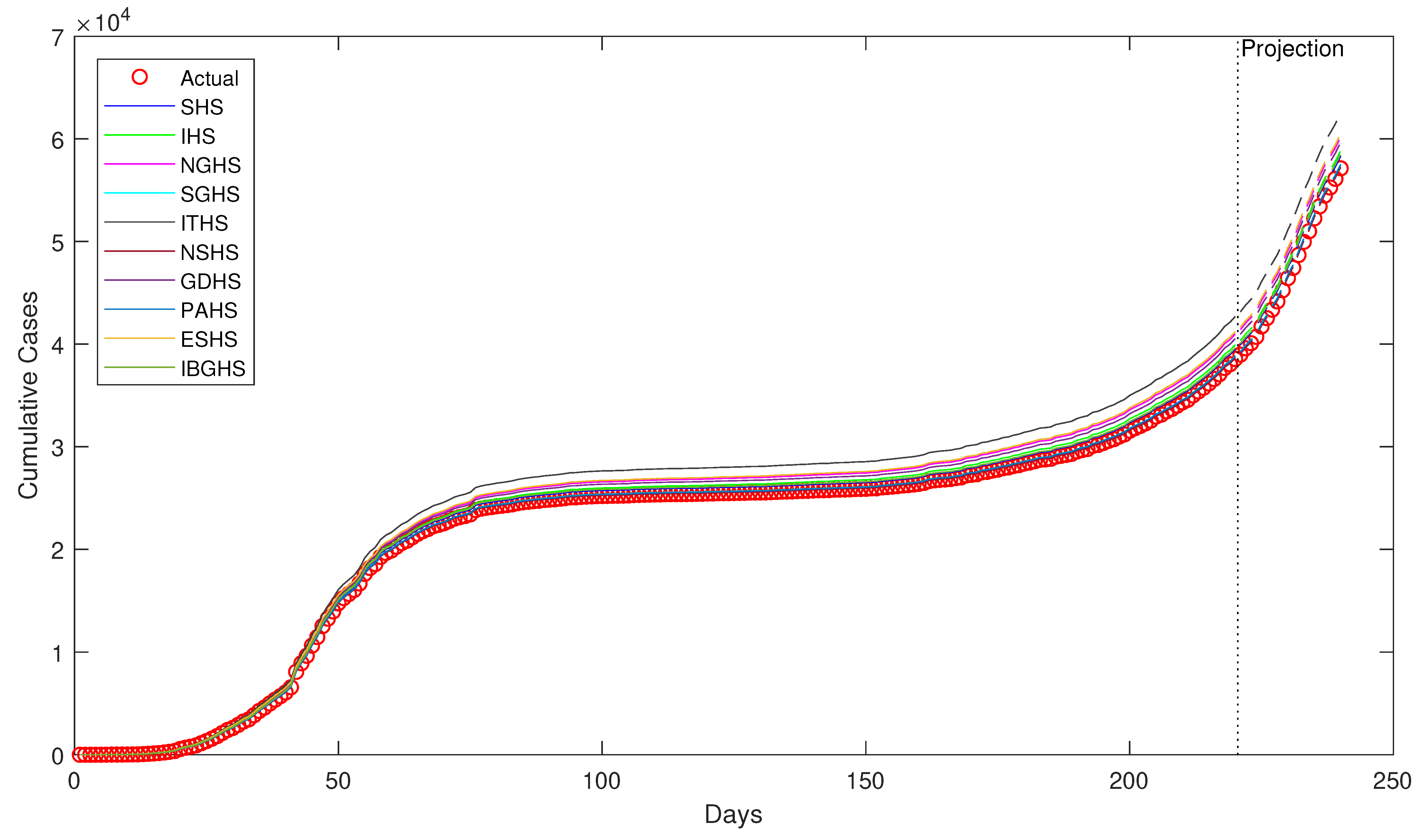
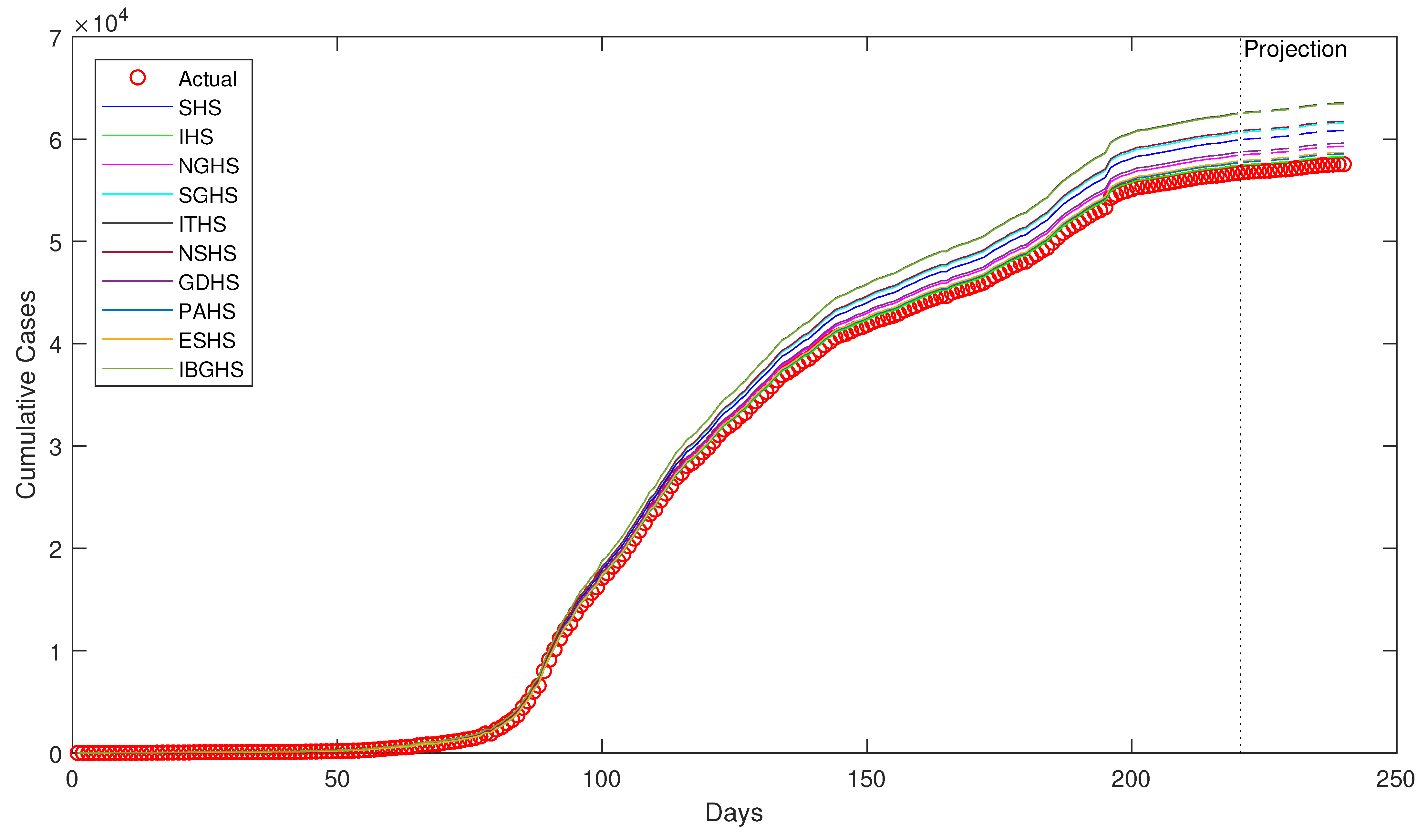
Despite being successfully applied in various fields, to the best of our knowledge, HS algorithms have yet to be applied in epidemiology, particularly in epidemiological modeling. Thus, in this study, ten variants of HS algorithm is proposed to be applied in order to estimate the epidemiological parameters of interest in the prototypical compartmental epidemiological SIR model and compare the estimation performance of each algorithm.

3. Estimating the Epidemiological Parameters of SIR Model

HS algorithms are applied to the SIR parameter estimation problem while using the cumulative infectious cases (total cases) of the COVID-19 pandemic as the use-case. The optimized (final) values of parameters $\beta$ and $\gamma$ are estimated by calibrating the available COVID-19 data and the SIR model with the generated harmonies (candidate solutions) from HM.

3.1. COVID-19 Data Sets

The authors obtain the time series of cumulative infectious cases per day for five countries, namely the United States of America (USA), France (FR), South Korea (SK), Ireland (IR), and Singapore (SG), by web scraping the figures in https://www.worldometers.info/coronavirus (which gathers data from various reliable sources including European Centre for Disease Prevention & Control and Johns Hopkins University & Medicine Coronavirus Resource Center). The data collected are for a period of 240 days, beginning from the first day of the outbreak in each country. Next, the first 220 days data is used for calibration to obtain the estimates of the parameters. The remaining 20 days of data are used for validation against the projection of simulation produced while using the HS optimized parameter values.

3.2. SIR Model Setup

The SIR compartments are initialized (at time $t=0$) with initial conditions $I_0\mathrm{and}{R}_0$, according to the actual number of infectious and removed cases, respectively, on the first day of the outbreak in each country. Meanwhile, $S_0$ is set as the remaining individuals in the population N who are yet to be infected and removed, i.e., $S_0=N-I_0-R_0$.

Table 1. Susceptible-Infectious-Removed (SIR) modeling initialization.

Data Set	Calibration Period	Projection Period	${\mathit{I}}_0$	${\mathit{R}}_0$	N *
(Country)	(220 Days)	(20 Days)
USA	21 January 2020–27 August 2020	28 August 2020–16 September 2020	1	0	331,002,651
FR	25 January 2020–31 August 2020	1 September 2020–20 September 2020	3	0	65,273,511
SK	20 January 2020–26 August 2020	27 August 2020–15 September 2020	1	0	51,269,185
IR	29 February 2020–5 October 2020	6 October 2020–25 October 2020	1	0	4,937,786
SG	24 January 2020–30 August 2020	31 August 2020–19 September 2020	3	0	5,850,342

* estimated at mid year according to UN data.

provides the modeling initialization.

3.3. SIR Parameters Estimation as Optimization Problem

The estimation of SIR parameters is formulated as an optimization problem with decision variables $\mathbf{x}=\{x_1,x_2\}$, where $\beta =x_1$ and $\gamma =x_2$. The upper and lower bounds of the decision variables are set according to the complete possible ranges of $\beta$ and $\gamma$, which are essentially the epidemiological dynamics’ rates and, hence, they share the same bounds, i.e., $\beta ,\gamma \in (0,1)$. The objective function is formulated, as follows:

• Let $C_T={\sum }_{t=0}^{t=T}{I}_t$ be the observed cumulative infectious cases on day $t=T,(t,T\in [0,219\left]\right)$, where $I_t$ is the observed infectious cases on day t.
• Let ${\widehat{C}}_T={\sum }_{t=0}^{t=T}{\widehat{I}}_t$ be the simulated cumulative infectious cases (rounded to the corresponding integers) on day $t=T,(t,T\in [0,219\left]\right)$, where ${\widehat{I}}_t$ is the SIR model simulated infectious cases on (rounded to the corresponding integers) day t while using $\mathbf{x}\in$ HM.
• Subsequently, an objective function $f(·)$ that minimizes the SSE between $C_T$ and ${\widehat{C}}_T$ can be formulated as:

  $$\mathrm{minimize}f\left(\mathbf{x}\right)=\sum _{T=0}^{T=219}{(C_T-{\widehat{C}}_T)}^2\mathrm{s}.\mathrm{t}\mathbf{x}\in (0,1).$$

  (22)

A set of ten independent runs is performed for each HS algorithm while using each of the data sets. The optimization steps are detailed, as follows:

• The common control parameters shared among all ten algorithms are set to be identical, $HMS=30$ and $MaxImp=50,000$, following the recommendation in [47].
• Ten initial HMs $(H{M}_1,H{M}_2,\cdots ,H{M}_{10})$ and ten corresponding initial fitness vectors $(f_1,f_2,\cdots ,f_{10})$ are generated to be used in each run according to the initialization of HM (Step 2) in Section 2.
• Optimization is performed for ten independent runs for each data set while using the identical $HM$ and f using each of the algorithms (Algorithm 1 to Algorithm 10), as described in Section 2. For instance, the first run for the USA data set will be performed while using the same $H{M}_1$ and $f_1$ for all ten HS algorithms. The specific control parameters that are shared among some algorithms are also set to be identical as displayed in

  Table 2. Specific control parameters of Harmony Search (HS) algorithms.

  Algorithm	HMCR	PAR	PAR	HMCRmin	HMCRmax	PARmin	PARmax	BWmin	BWmax	Pm	Pc	LP	HMCRm	PARm
  SHS	0.95	0.3	0.01	-	-	-	-	-	-	-	-	-	-	-
  IHS	0.95	-	-	-	-	0.99	0.01	0.001	1/(20x(UB-LB))	-	-	-	-	-
  NGHS	-	-	-	-	-	-	-	-	-	0.005	-	-	-	-
  SGHS	-	-	-	-	-	-	-	0.001	1/(20x(UB-LB))	-	-	100	0.98	0.9
  ITHS	0.95	-	-	-	-	0.99	0.01	-	-	-	-	-	-	-
  NSHS	-	-	-	-	-	-	-	-	-	-	-	-	-	-
  GDHS	-	-	-	-	-	-	-	-	-	-	-	-	-	-
  PAHS	-	-	-	0.99	0.7	0.99	0.01	0.001	1/(20x(UB-LB))	-	-	-	-	-
  ESHS	-	-	-	-	-	-	-	-	-	-	-	-	-	-
  IBGHS	-	0.3	0.01	-	-	-	-	-	-	0.005	0.9	-	-	-

  .
• Repeat Step 3 until the runs are completed for all five data sets. The combination of parameters’ values that yields the best fitness (lowest SSE) are designated as the optimized parameters.
• The average values of $\{{\mathbf{x}}_1,{\mathbf{x}}_2\}=\{{\overline{x}}_1,{\overline{x}}_2\}$ from each run for each HS algorithm are obtained, where,

  $${\overline{x}}_i=\frac{{\sum }_{k=1}^{k=10}{x}_{ik}}{10},(i=1,2),(k=1,2,\dots ,10).$$

  (23)
  Subsequently, $\{{\overline{x}}_1,{\overline{x}}_2\}$ are designated as the overall optimized SIR parameters with respect to each algorithm, thus ${\mathbf{x}}_{optimized}=\{{\overline{x}}_1,{\overline{x}}_2\}$. Note that the identical common and specific control parameters, as well as the identical HM and f, are used in this study to ensure a fair comparison among the HS algorithms.

3.4. Evaluation of HS Estimation and Performance Comparison

The accuracy of the SIR parameter estimates is deduced from the fitness values (SSE), where the algorithm with lowest fitness is designated as the best performing estimator and vice-versa. The optimized epidemiological parameters ${\mathbf{x}}_{optimized}$ are supplied to the SIR model once again to produce a projection of simulation for a period of 20 subsequent days from the end date of calibration period in order to evaluate the predictive capability of SIR model while using the parameters that were estimated from HS algorithms. Let $C_T$ be the observed cumulative infectious cases on the projection period and ${\widehat{C}}_T$ be the projected SIR model simulated cumulative infectious cases using ${\mathbf{x}}_{optimized}$, then the accuracy of estimation is evaluated by computing the Root Mean Squared Error (RMSE) between $C_T$ and ${\widehat{C}}_T$ in the period of projection using:

$$RMSE=\sqrt{\frac{{\sum }_{T=220}^{T=239}{(C_T-{\widehat{C}}_T)}^2}{20}}.$$

(24)

The accuracy of the SIR model’s projected simulation is decided based on the RMSE value, where a lower RMSE value indicates a better prediction and vice-versa. Eventually, the predictive capability indicates the parameter estimation accuracy of the HS variants. The corresponding RMSE for each algorithm within the same data set will be statistically compared. The comparison is performed while using the Friedman test to see whether there is an overall significant difference in the estimations produced by each of the algorithms. Furthermore, if the performance of SHS is found to be comparable with the rest of the HS variants, then the post-hoc procedure of Wilcoxon signed-rank tests is conductedin order tto determine whether there is any statistically significant difference between the estimation performance of SHS and the rest of the HS variants individually.

4. SIR Simulation Experiments and Discussion

In this section, SIR simulation experiments are performed to illustrate the ability of HS algorithms as an efficacious estimator of SIR parameters. All of the variants of HS algorithm were coded in MATLAB R2017b on a laptop computer with 2.50 GHz Intel i7–4710HQ CPU with 32 GB of RAM. The discussion is discretely presented for each data set used in this study.

4.1. Simulations and Projected Simulations

4.1.1. USA Data Set (United States of America)

Table 3. USA: Optimized parameters and corresponding fitness.

Algorithm	${\mathit{x}}_{\mathbf{1}}\mathbf{\left(}\mathit{\beta }\mathbf{\right)}$	${\mathit{x}}_{\mathbf{2}}\mathbf{\left(}\mathit{\gamma }\mathbf{\right)}$	$\mathit{f}\mathbf{\left(}\mathbf{x}\mathbf{\right)}$ (SSE)
SHS	0.4208	0.0931	1098.33
IHS	0.4198	0.0938	1072.83
NGHS	0.4212	0.0924	1174.67
SGHS	0.4202	0.0934	1076.62
ITHS	0.4203	0.0933	1082.46
NSHS	0.4202	0.0934	1077.16
GDHS	0.4202	0.0934	1077.14
PAHS	0.4198	0.0938	1073.06
ESHS	0.4202	0.0934	1077.22
IBGHS	0.4210	0.0921	1132.08

presents the optimized epidemiological parameters and corresponding fitness values (average from ten independent runs) for the USA data set. Figure 2 displays the visualization of the 220 days simulation together with the 20 days projected simulation using the optimized parameters. Visual inspection for USA data set is not informative enough as some of the lines representing the algorithms overlapped, which suggested that the estimates are very close to each other, except for NGHS, IBGHS, SHS, ITHS, ESHS, PAHS, and IHS that are visible. Simulations of each algorithms for approximately the first 100 days were indeed close to each other as well as to the observed cumulative cases. Beginning from the hundredth day of the outbreak, the simulations of each algorithm showed differences while they started deviating from the observed values, except for PAHS and IHS, which are still intact with the observed values. The projected simulation for subsequent 20 days were consistent in terms of the pattern in the calibration period. It is observed from the fitness values (SSE) in Table 3 that IHS appears to be the best performing estimator for USA data set, while NGHS is the least performing estimator.

For the USA data set, it is observed that the simulation from each HS algorithms are not very far off the observed cumulative cases, even in the projection period. Most of the simulations are similar as far as the parameters’ values are concerned and they were able to approximately resemble the observed trend. Simulations of NGHS and IBGHS are the farthest deviation from the actual values. The similar behavior between these two algorithms may be due to the use of genetic mutation in the improvisation step that sets them apart from the rest of the algorithms.

4.1.2. FR Data Set (France)

Table 4. FR: Optimized parameters and corresponding fitness.

Algorithm	${\mathit{x}}_{\mathbf{1}}\mathbf{\left(}\mathit{\beta }\mathbf{\right)}$	${\mathit{x}}_{\mathbf{2}}\mathbf{\left(}\mathit{\gamma }\mathbf{\right)}$	$\mathit{f}\mathbf{\left(}\mathbf{x}\mathbf{\right)}$ (SSE)
SHS	0.2208	0.1227	1002.11
IHS	0.2221	0.1223	1211.77
NGHS	0.2224	0.1220	1427.31
SGHS	0.2213	0.1225	1101.25
ITHS	0.2214	0.1226	1102.71
NSHS	0.2213	0.1226	1102.42
GDHS	0.2208	0.1228	992.04
PAHS	0.2218	0.1226	1125.00
ESHS	0.2218	0.1226	1125.36
IBGHS	0.2207	0.1228	987.31

provides the optimized epidemiological parameters and the corresponding fitness values (the average from 10 independent runs) for the FR data set. The visualization of the 220 days simulation together with the 20 days projected simulation using the optimized parameters are depicted in Figure 3. The simulations can be visually inspected as the lines representing the algorithms do not overlap each other except for SHS, which overlaps with GDHS. During the calibration period the simulation of IHS was similar but not so close to ESHS and PAHS. However, in the projection period, IHS’s simulation seems to be closer to ESHS and PAHS. The other groups of algorithms that produced similar simulations are ITHS, NSHS, SGHS and SHS, GDHS, IBGHS. The simulations started diverging from each after day 60 of the outbreak, and gradually digressed from the observed cumulative values all the way up to the projection period. The projected simulation for subsequent 20 days depicted a further deviance of the simulations from the observed values. It is observed from the fitness values (SSE) in Table 4, that IBGHS appears to best performing estimator for FR data set, while NGHS is the least performing estimator, just as the case of USA data set.

For the FR data set, observe that the simulations are slightly far off the observed cumulative cases. The simulations were not able to accurately mimic the observed trend. NGHS’s simulation was apart all the way, whereas we can infer that the simulations of IHS, ESHS, and PAHS are similar; ITHS, NSHS, and SGHS are alike; and finally, SGHS, GDHS, SHS, and IBGHS are close to each other. NGHS’s simulation is again the farthest and different from the rest, which is probably due to the use of genetic mutation, which sets it apart from the rest. Genetic mutation is also used in IBGHS, but the standard $PAR$ setting in IBGHS could have contributed to the high similarity in behavior as SHS than NGHS. Hence, for this particular data set, the $PAR$ parameter was more influential then genetic mutation, as compared to the USA data set.

4.1.3. SK Data Set (South Korea)

Table 5. SK: Optimized parameters and corresponding fitness.

Algorithm	${\mathit{x}}_{\mathbf{1}}\mathbf{\left(}\mathit{\beta }\mathbf{\right)}$	${\mathit{x}}_{\mathbf{2}}\mathbf{\left(}\mathit{\gamma }\mathbf{\right)}$	$\mathit{f}\mathbf{\left(}\mathbf{x}\mathbf{\right)}$ (SSE)
SHS	0.3125	0.1012	2382.52
IHS	0.3137	0.1011	2510.07
NGHS	0.3142	0.1014	2531.25
SGHS	0.3120	0.1013	2203.09
ITHS	0.3140	0.1012	2172.45
NSHS	0.3137	0.1011	2508.21
GDHS	0.3130	0.1012	2500.66
PAHS	0.3140	0.1014	2528.17
ESHS	0.3125	0.1011	2381.76
IBGHS	0.3135	0.1012	2504.14

presents the optimized epidemiological parameters and the corresponding fitness values (average from 10 independent runs) for the SK data set. Figure 4 displays the visualization of the 220 days simulation, together with the 20 days projected simulation using the optimized parameters. The simulations can be well visualized as the lines representing each algorithm is distinct, except for SHS, which overlaps with ESHS. The simulations started departing from the observed cumulative cases as early as the fiftieth day of the outbreak. The band of simulations also started deviating around the same time and was gradually separated up to the projection period. All of the simulations were distinguishable, except in the case of IHS and NSHS, which were close to each other and SHS and ESHS that were similar. The projected simulation for subsequent 20 days indicated a larger deviation of the simulations from the observed values. We observe from the fitness values (SSE) in Table 5 that ITHS appears to be the best performing estimator for SK data set, while NGHS is the least performing estimator, just as the case of USA and FR data sets.

For the SK data set, observe that the simulations are quite far off the observed cumulative cases, with NGHS being the farthest and ITHS being the nearest. Yet, ITHS’s simulation is still far off the observed cumulative cases comparatively. The simulations were not able to resemble the observed trend well. The simulation for SK data set is clearly not as good as USA or FR data sets. the simulations of all the algorithms were distinct except for the overlapping SHS and ESHS. NGHS’s simulation is again very different from the rest, probably due to use of genetic mutation, which sets it apart from the rest. As far as this data set is concerned, it is also interesting to observe ESHS that requires zero parameter setting and uses Gaussian mutation in the place of random generation of harmony, behaves somewhat similar to SHS.

4.1.4. IR Data Set (Ireland)

Table 6. IR: Optimized parameters and corresponding fitness.

Algorithm	${\mathit{x}}_{\mathbf{1}}\mathbf{\left(}\mathit{\beta }\mathbf{\right)}$	${\mathit{x}}_{\mathbf{2}}\mathbf{\left(}\mathit{\gamma }\mathbf{\right)}$	$\mathit{f}\mathbf{\left(}\mathbf{x}\mathbf{\right)}$ (SSE)
SHS	0.3426	0.1044	970.02
IHS	0.3427	0.1044	1078.34
NGHS	0.3436	0.1042	1233.88
SGHS	0.3425	0.1043	703.22
ITHS	0.3441	0.1042	1827.38
NSHS	0.3420	0.1043	662.22
GDHS	0.3432	0.1043	1202.47
PAHS	0.3425	0.1043	701.58
ESHS	0.3436	0.1041	1247.19
IBGHS	0.3425	0.1044	971.54

provides the optimized epidemiological parameters and the corresponding fitness values (average from 10 independent runs) for the IR data set. Figure 5 depicts the visualization of the 220 days simulation, together with the 20 days projected simulation using the optimized parameters. The visual inspection of the simulations is informative, although the lines representing most of the algorithms are quite close to each other, with only SGHS and PAHS overlapping. The simulations drifted away from the observed cumulative cases as early as before the fiftieth day of the outbreak itself. However, the simulations of SGHS, PAHS, and NSHS managed to stay intact with the observed values, even during the projection period. On the other hand, the simulations of IHS, IBGHS, and SHS were still close to the observed values and they became closer in the projection period. ITHS remained steadily far from the observed values, while ESHS, NGHS, and GDHS maintained a constant separation from the observed values. The projected simulation for subsequent 20 days indicated a smaller deviation of the simulations from the observed values, except for ITHS. It is observed from the fitness values (SSE) in Table 6 that NSHS appears to be the best performing estimator for IR data set, while ITHS emerged as the least performing estimator.

For the IR data set, it is observed that the simulations are reasonably close to the observed cumulative cases, except for ITHS. This shows that most of the simulations managed to mimic the observed trend well. Excluding ITHS, we can group the algorithms with similar simulations as (i) ESHS, NGHS, and GDHS; (ii) IHS, IBGHS, and SHS; and, (iii) SGHS, PAHS, and NSHS. Note that the difference in the simulation of ITHS was better in the previous three data sets, but it appeared to be the worst in this data set. The combination of algorithms that produced similar simulations is also different from combinations in previous data set, notably the FR data set.

4.1.5. SG Data Set (Singapore)

Table 7. SG: Optimized parameters and corresponding fitness.

Algorithm	${\mathit{x}}_{\mathbf{1}}\mathbf{\left(}\mathit{\beta }\mathbf{\right)}$	${\mathit{x}}_{\mathbf{2}}\mathbf{\left(}\mathit{\gamma }\mathbf{\right)}$	$\mathit{f}\mathbf{\left(}\mathbf{x}\mathbf{\right)}$ (SSE)
SHS	0.3604	0.1331	2015.77
IHS	0.3582	0.1334	1002.64
NGHS	0.3600	0.1332	1799.32
SGHS	0.3607	0.1331	2238.65
ITHS	0.3612	0.1328	2564.23
NSHS	0.3608	0.1331	2241.29
GDHS	0.3600	0.1333	1805.79
PAHS	0.3585	0.1333	1542.52
ESHS	0.3588	0.1332	1622.38
IBGHS	0.3611	0.1328	2557.87

provides the optimized epidemiological parameters and the corresponding fitness values (average from 10 independent runs) for the SG data set. Figure 6 displays the visualization of the 220 days simulation, together with the 20 days projected simulation using the optimized parameters. The simulations are distinguishable, thus the visualization is informative, except for a slight overlap between ITHS and IBGHS. The simulations band begin to diverge from the observed cumulative cases approximately around the hundredth day of the outbreak, except for the simulations of ESHS, PAHS, and IHS, which diverged gradually. While other simulations deviated from the rest, ESHS, PAHS, and IHS were close to each other until day 200 of the outbreak. Only after that, the simulations diverged from each other in a small amount up to the projection period. All of the simulations were far from the observed values, resembling a similarity with the case of simulations in the SK data set. The projected simulation for subsequent 20 days indicated an even larger deviation of the simulations from the observed values. It is observed from the fitness values (SSE) presented in Table 7 that IHS appears to best performing estimator for SG data set, while ITHS is the least performing estimator, similar to IR data set.

For the SG data set, it is observed that the simulations are quite far off the actual cumulative cases, with ITHS being the farthest and IHS being the nearest. Nevertheless, IHS’s simulation is still far off the observed cumulative cases. The simulations were not able to resemble the observed trend well and it is undoubtedly not as good as for USA, FR, and IR data sets. The quality of simulations are similar to the SK data set. The simulations of ITHS and IBGHS are really far off the observed values. We note that the simulations of ITHS and IBGHS are similar, NSHS and SGHS are close to each other, GDHS and NGHS are approximately close, ESHS and PAHS are close to each other, while SHS and IHS were not similar or close to the rest.

4.2. Performance Comparison

Following the SIR simulation experiments that were performed on the five data sets, it is noted that the performance of each algorithm (based on the fitness values (SSE)) varies across the data sets. Based on the parameter estimates for each data set presented in Table 3, Table 4, Table 5, Table 6 and Table 7, the estimates produced by each algorithm are fairly similar, which indicates that the optimization performed is consistent due to the underlying nature of HS, regardless of the type of HS variant.

Table 8. Best performing algorithm for each data set.

Data Set	Best Algorithm
USA	IHS
FR	IBGHS
SK	ITHS
IR	NSHS
SG	IHS

lists the best performing algorithm for each data set. Apparently, there is no one clear winner algorithm for this particular application of HS.

We obtain the RMSE values from the 20 days projected SIR simulation while using Equation (24) in order to statistically compare the performance of each algorithm within each of the data sets. The Friedman test is conducted to determine whether there is any statistically significant differences among the estimation performances (in terms of RMSE) of each algorithm.

Table 9. RMSE.

Algorithm	USA	FR	SK	IR	SG
SHS	25.39	12.86	29.73	16.66	28.44
IHS	12.95	18.73	34.12	18.55	17.23
NGHS	38.12	27.32	39.64	25.44	24.22
SGHS	13.85	13.63	26.24	13.45	30.66
ITHS	15.34	14.75	25.44	37.89	39.14
NSHS	14.76	14.28	34.08	10.98	31.28
GDHS	14.22	12.19	33.64	22.62	25.22
PAHS	13.02	16.38	30.08	13.03	19.86
ESHS	14.92	16.59	38.7	26.12	21.46
IBGHS	33.69	11.35	33.78	16.94	38.37

displays the RMSE values.

The low RMSE values within each data set indicates that the predictive capability of SIR model while using the HS optimized parameters are fairly good. Eventually, it attests that the parameter estimation accuracy of HS variants is satisfactory. The Friedman test elicited no statistically significant difference in the estimation performance of the HS algorithms at significance level of 0.05 (${\chi }^2\left(9\right)=11.749,p=0.228$). It is noteworthy to observe that the estimation performance of SHS is comparable with the rest of the HS variants and fairly consistent across the data sets. The simulations of SHS are also reasonably close to the observed cumulative cases in FR, SK, IR, SG, and USA data sets (in the closest order). The post-hoc analysis for SHS is performed using the Wilcoxon signed-rank tests in order to identify whether there is any statistically significant difference between the estimation performance of SHS and the rest of the HS variants individually.

Table 10. Post-hoc analysis for standard HS (SHS).

Test	Z	p-Value
SHS–IHS	$-0.405$	0.686
SHS–NGHS	$-1.753$	0.080
SHS–SGHS	$-1.214$	0.225
SHS–ITHS	$-0.674$	0.500
SHS–NSHS	$-0.405$	0.686
SHS–GDHS	$-0.135$	0.893
SHS–PAHS	$-1.214$	0.225
SHS–ESHS	$-0.135$	0.893
SHS–IBGHS	$-1.483$	0.138

displays the test results.

The Wilcoxon signed-rank tests that were conducted with a Bonferroni correction applied at the resulting significance level of $\frac{0.05}{9}=0.006$ elicited no statistically significant difference in the estimation performance of SHS when compared to the rest of the HS variants individually. Indeed, the insignificant difference supports that the performance of SHS is comparable. Therefore, although SHS may not be the best performing algorithm for any of the data sets, the consistency and statistical tests’ results elucidate that SHS is competent enough to be a potential efficacious estimator for the epidemiological parameters of SIR model. A slight manual fine-tuning of the control parameters may do the job of increasing the estimation accuracy of SHS. In essence, the primary advantages of applying HS to estimate the epidemiological parameters of compartmental models are as follows:

• No initial values for the epidemiological parameters are required. One does not need to adapt the values of epidemiological parameters from previous studies, so as to alleviate any bias in the estimation process.
• No specified upper and lower bounds for the epidemiological parameters are required to suit the data sets. The burdensome process of finding an appropriate range of the parameters for each data set are evaded by using the complete range of the parameters, regardless of the data set. This may increase the computational time, but it can be traded off with better computing resources.
• No in-depth information about the infectious disease is necessary. HS optimization can well be applied to other infectious disease modeling without extra specific information about the disease.

5. Conclusions and Future Work

The application of HS is a novel approach in the field of epidemiology, particularly in epidemiological modeling. In this study, HS was implemented in order to estimate the epidemiological parameters of the prototypical compartmental SIR model as an optimization problem. Ten variants of HS algorithm were applied on five data sets to simulate the trajectory of COVID-19 cumulative infectious cases. The computational experiments demonstrated the ability of HS to be successfully applied to epidemiological modeling and as an efficacious estimator for the model parameters. As such, HS is proposed as a potential alternative estimation tool for the epidemiological parameters. An interesting insight from this study is that SHS is competent enough and it exhibited comparable performance with the rest of the HS variants in this particular application of HS optimization. For future work, the application of HS can be expanded to parameter estimations in advanced compartmental epidemiological models (e.g.,: SEIR model) and to the modeling of other existing infectious diseases (e.g.,: H1N1) or potential novel infectious diseases in the future.

References

1. Thompson, R.N. Epidemiological models are important tools for guiding COVID-19 interventions. BMC Med. 2020, 18, 152. [Google Scholar] [CrossRef] [PubMed]
2. Viboud, C.; Sun, K.; Gaffey, R.; Ajelli, M.; Fumanelli, L.; Merler, S.; Zhang, Q.; Chowell, G.; Simonsen, L.; Vespignani, A.; et al. The RAPIDD ebola forecasting challenge: Synthesis and lessons learnt. Epidemics 2018, 22, 13–21. [Google Scholar] [CrossRef] [PubMed]
3. Cooper, B.S.; Pitman, R.J.; Edmunds, W.J.; Gay, N.J. Delaying the international spread of pandemic influenza. PLoS Med. 2006, 3, e212. [Google Scholar] [CrossRef] [PubMed]
4. Kucharski, A.J.; Camacho, A.; Checchi, F.; Waldman, R.; Grais, R.F.; Cabrol, J.C.; Briand, S.; Baguelin, M.; Flasche, S.; Funk, S.; et al. Evaluation of the benefits and risks of introducing Ebola community care centers, Sierra Leone. Emerg. Infect. Dis. 2015, 21, 393–399. [Google Scholar] [CrossRef] [PubMed]
5. Aylward, B.; Barboza, P.; Bawo, L.; Bertherat, E.; Bilivogui, P.; Blake, I.; Brennan, R.; Briand, S.; Chakauya, J.M.; Chitala, K.; et al. Ebola virus disease in West Africa–the first 9 months of the epidemic and forward projections. N. Engl. J. Med. 2014, 371, 1481–1495. [Google Scholar]
6. Kucharski, A.J.; Timothy, W.R.; Charlie, D.; Yang, L.; John, E.; Sebastian, F.; Rosalind, M.E.; Centre for Mathematical Modelling of Infectious Diseases COVID-19 Working Group. Early dynamics of transmission and control of COVID-19: A mathematical modelling study. Lancet Infect Dis. 2020, 20, 553–558. [Google Scholar] [CrossRef] [Green Version]
7. Egger, M.; Johnson, L.; Althaus, C.; Schöni, A.; Salanti, G.; Low, N.; Norris, S. Developing WHO guidelines: Time to formally include evidence from mathematical modelling studies. F1000Research 2017, 6, 1584. [Google Scholar] [CrossRef]
8. Jewell, N.P.; Lewnard, J.A.; Jewell, B.L. Predictive mathematical models of the COVID-19 pandemic: Underlying principles and value of projections. JAMA 2020, 323, 1893–1894. [Google Scholar] [CrossRef]
9. Adam, D. Special report: The simulations driving the world’s response to covid-19. Nature 2020, 580, 316–318. [Google Scholar] [CrossRef] [Green Version]
10. Chen, D.; Moulin, B.; Wu, J. Analyzing and Modeling Spatial and Temporal Dynamics of Infectious Diseases; John Wiley & Sons: Hoboken, NJ, USA, 2014. [Google Scholar]
11. Abou-Ismail, A. Compartmental models of the COVID-19 pandemic for physicians and physician-scientists. SN Compr. Clin. Med. 2020, 2, 852–858. [Google Scholar] [CrossRef]
12. Wang, L.; Zhou, Y.; He, J.; Zhu, B.; Wang, F.; Tang, L.; Kleinsasser, M.; Barker, D.; Eisenberg, M.C.; Song, X.K. An epidemiological forecast model and software assessing interventions on the COVID-19 epidemic in China. J. Data Sci. 2020, 8, 409–432. [Google Scholar]
13. Wangping, J.; Ke, H.; Yang, S.; Wenzhe, C.; Shengshu, W.; Shanshan, Y.; Jianwei, W.; Fuyin, K.; Penggang, T.; Jing, L.; et al. Extended SIR prediction of the epidemics trend of COVID-19 in Italy and compared with Hunan, China. Front. Med. 2020, 7, 169. [Google Scholar] [CrossRef] [PubMed]
14. Tang, B.; Wang, X.; Li, Q.; Bragazzi, N.L.; Tang, S.; Xiao, Y.; Wu, J. Estimation of the transmission risk of the 2019-nCoV and its implication for public health interventions. J. Clin. Med. 2020, 9, 462. [Google Scholar] [CrossRef] [PubMed] [Green Version]
15. Rocchi, E.; Peluso, S.; Sisti, D.; Carletti, M. A possible scenario for the Covid-19 epidemic, based on the SI (R) model. SN Compr. Clin. Med. 2020, 2, 501–503. [Google Scholar] [CrossRef]
16. Wu, J.T.; Leung, K.; Leung, G.M. Nowcasting and forecasting the potential domestic and international spread of the 2019-nCoV outbreak originating in Wuhan, China: A modelling study. Lancet 2020, 395, 689–697. [Google Scholar] [CrossRef] [Green Version]
17. Choi, S.; Ki, M. Estimating the reproductive number and the outbreak size of COVID-19 in Korea. Epidemiol. Health 2020, 42, e2020011. [Google Scholar] [CrossRef]
18. Verity, R.; Okell, L.C.; Dorigatti, I.; Winskill, P.; Whittaker, C.; Imai, N.; Cuomo-Dannenburg, G.; Thompson, H.; Walker, P.G.T.; Fu, H.; et al. Estimates of the severity of coronavirus disease 2019: A model-based analysis. Lancet Inf. Dis. 2020, 20, 669–677. [Google Scholar] [CrossRef]
19. Mohamadou, Y.; Halidou, A.; Kapen, P.T. A review of mathematical modeling, artificial intelligence and datasets used in the study, prediction and management of COVID-19. Appl. Intell. 2020, 50, 3913–3925. [Google Scholar] [CrossRef]
20. Thompson, R.N.; Hollingsworth, T.D.; Isham, V.; Arribas-Bel, D.; Ashby, B.; Britton, T.; Challenor, P.; Chappell, L.H.K.; Clapham, C.H.; Cunniffe, N.J.; et al. Key questions for modelling COVID-19 exit strategies. Proc. R. Soc. B 2020, 287, 20201405. [Google Scholar] [CrossRef]
21. Ridenhour, B.; Kowalik, J.M.; Shay, D.K. Unraveling R0: Considerations for public health applications. Am. J. Public Health 2018, 108, S445–S454. [Google Scholar] [CrossRef]
22. Tang, L.; Zhou, Y.; Wang, L.; Purkayastha, S.; Zhang, L.; He, J.; Wang, F.; Song, P.X.K. A Review of Multi-Compartment Infectious Disease Models. Int. Stat. Rev. 2020, 88, 462–513. [Google Scholar] [CrossRef] [PubMed]
23. Su, L.; Hong, N.; Zhou, X.; He, J.; Ma, Y.; Jiang, H.; Han, L.; Chang, F.; Shan, G.; Zhu, W.; et al. Evaluation of the secondary transmission pattern and epidemic prediction of COVID-19 in the four metropolitan areas of China. Front. Med. 2020, 7, 556366. [Google Scholar] [CrossRef] [PubMed]
24. Akman, O.; Schaefer, E. An evolutionary computing approach for parameter estimation investigation of a model for cholera. J. Biol. Dyn. 2015, 9, 147–158. [Google Scholar] [CrossRef] [PubMed] [Green Version]
25. Akman, O.; Corby, M.R.; Schaefer, E. Examination of models for cholera: Insights into model comparison methods. Lett. Biomath. 2016, 3, 93–118. [Google Scholar] [CrossRef]
26. Tutkun, N. Parameter estimation in mathematical models using the real coded genetic algorithms. Expert Syst. Appl. 2009, 36, 3342–3345. [Google Scholar] [CrossRef]
27. Akman, D.; Akman, O.; Schaefer, E. Parameter estimation in ordinary differential equations modeling via particle swarm optimization. J. Appl. Math. 2018, 2018, 9160793. [Google Scholar] [CrossRef] [Green Version]
28. Alsayed, A.; Sadir, H.; Kamil, R.; Sari, H. Prediction of epidemic peak and infected cases for COVID-19 disease in Malaysia, 2020. Int. J. Environ. Res. Public Health 2020, 17, 4076. [Google Scholar] [CrossRef]
29. Makade, R.G.; Chakrabarti, S.; Jamil, B. Real-time estimation and prediction of the mortality caused due to COVID-19 using particle swarm optimization and finding the most influential parameter. Infect. Dis. Model. 2020, 5, 772–782. [Google Scholar] [CrossRef]
30. Godio, A.; Pace, F.; Vergnano, A. SEIR modeling of the Italian epidemic of SARS-CoV-2 using computational swarm intelligence. Int. J. Environ. Res. Public Health 2020, 17, 3535. [Google Scholar] [CrossRef]
31. Lobato, F.S.; Libotte, G.B.; Platt, G.M. Identification of an epidemiological model to simulate the COVID-19 epidemic using robust multiobjective optimization and stochastic fractal search. Comput. Math. Methods Med. 2020, 2020, 9214159. [Google Scholar] [CrossRef]
32. Al-Qaness, M.A.A.; Ewees, A.A.; Fan, H.; Abualigah, L.; Abd Elaziz, M. Marine predators algorithm for forecasting confirmed cases of COVID-19 in Italy, USA, Iran and Korea. Int. J. Environ. Res. Public Health 2020, 17, 3520. [Google Scholar] [CrossRef] [PubMed]
33. Al-Qaness, M.A.A.; Ewees, A.A.; Fan, H.; Abd El Aziz, M. Optimization method for forecasting confirmed cases of COVID-19 in China. J. Clin. Med. 2020, 9, 674. [Google Scholar] [CrossRef] [Green Version]
34. Geem, Z.W.; Kim, J.H.; Loganathan, G.V. A new heuristic optimization algorithm: Harmony search. Simulation 2001, 76, 60–68. [Google Scholar] [CrossRef]
35. Yi, J.; Lu, C.; Li, G. A literature review on latest developments of Harmony Search and its applications to intelligent manufacturing. Math. Biosci. Eng. 2019, 16, 2086–2117. [Google Scholar] [CrossRef] [PubMed]
36. Goh, R.Y.; Lee, L.S.; Seow, H.V.; Gopal, K. Hybrid harmony search-artificial intelligence models in credit scoring. Entropy 2020, 22, 989. [Google Scholar] [CrossRef] [PubMed]
37. Al-Omoush, A.A.; Alsewari, A.; Alamri, H.S.; Zamli, K.Z. Comprehensive review of the development of the harmony search algorithm and its applications. IEEE Access 2019, 7, 14233–14245. [Google Scholar] [CrossRef]
38. Misni, F.; Lee, L.S.; Seow, H.V. Hybrid harmony search-simulated annealing algorithm for location-inventory-routing problem in supply chain network design with defect and non-defect items. Appl. Sci. 2020, 10, 6625. [Google Scholar] [CrossRef]
39. Moh’d Alia, O.; Mandava, R. The variants of the harmony search algorithm: An overview. Artif. Intell. Rev. 2011, 36, 49–68. [Google Scholar] [CrossRef]
40. Kim, J.H.; Geem, Z.W.; Kim, E.S. Parameter estimation of the nonlinear muskingum model using harmony search. JAWRA J. Am. Water Resour. Assoc. 2001, 37, 1131–1138. [Google Scholar] [CrossRef]
41. Geem, Z.W. Parameter estimation of the nonlinear Muskingum model using parameter-setting-free harmony search. J. Hydrol. Eng. 2011, 16, 684–688. [Google Scholar] [CrossRef]
42. Bonilla-Petriciolet, A.; Segovia-Hernández, J.G.; Soto-Bernal, J.J. Harmony search for parameter estimation in vapor-liquid equilibrium modeling. In Proceedings of the 5th International Symposium on Design, Operation and Control of Chemical Processes, Singapore, 25–28 July 2010; pp. 719–726. [Google Scholar]
43. Chun, H.; Kim, M.; Kim, J.; Kim, K.; Yu, J.; Kim, T.; Han, S. Adaptive exploration harmony search for effective parameter estimation in an electrochemical lithium-ion battery model. IEEE Access 2019, 7, 131501–131511. [Google Scholar] [CrossRef]
44. Zhang, W.; Li, W.; Zhang, J.; Wang, N. Optimal parameter identification of synthetic gene networks using harmony search algorithm. PLoS ONE 2019, 14, e0213977. [Google Scholar] [CrossRef] [PubMed] [Green Version]
45. Yoon, S.; Jeong, C.; Lee, T. Application of harmony search to design storm estimation from probability distribution models. J. Appl. Math. 2013, 2013, 932943. [Google Scholar] [CrossRef]
46. Fairchild, G.; Hickmann, K.S.; Mniszewski, S.M.; Del Valle, S.Y.; Hyman, J.M. Optimizing human activity patterns using global sensitivity analysis. Comput. Math. Organ. Theory 2014, 20, 394–416. [Google Scholar] [CrossRef] [Green Version]
47. Zhang, T.; Geem, Z.W. Review of harmony search with respect to algorithm structure. Swarm Evol. Comput. 2019, 48, 31–43. [Google Scholar] [CrossRef]
48. Siddique, N.; Adeli, H. Harmony search algorithm and its variants. Int. J. Pattern Recognit. Artif. Intell. 2015, 29, 1539001. [Google Scholar] [CrossRef]
49. Manjarres, D.; Landa-Torres, I.; Gil-Lopez, S.; Del Ser, J.; Bilbao, M.N.; Salcedo-Sanz, S.; Geem, Z.W. A survey on applications of the harmony search algorithm. Eng. Appl. Artif. Intell. 2013, 26, 1818–1831. [Google Scholar] [CrossRef]
50. Mahdavi, M.; Fesanghary, M.; Damangir, E. An improved harmony search algorithm for solving optimization problems. Appl. Math. Comput. 2007, 188, 1567–1579. [Google Scholar] [CrossRef]
51. Luo, K. A novel self-adaptive harmony search algorithm. J. Appl. Math. 2013, 2013, 653749. [Google Scholar] [CrossRef]
52. Omran, M.G.H.; Mahdavi, M. Global-best harmony search. Appl. Math. Comput. 2008, 198, 643–656. [Google Scholar] [CrossRef]
53. Wang, C.M.; Huang, Y.F. Self-adaptive harmony search algorithm for optimization. Expert Syst. Appl. 2010, 37, 2826–2837. [Google Scholar] [CrossRef]
54. Zou, D.; Liqun, G.; Jianhua, W.; Steven, L. Novel global harmony search algorithm for unconstrained problems. Neurocomputing 2010, 73, 3308–3318. [Google Scholar] [CrossRef]
55. Pan, Q.K.; Suganthan, P.N.; Tasgetiren, M.F.; Liang, J.J. A self-adaptive global best harmony search algorithm for continuous optimization problems. Appl. Math. Comput. 2010, 216, 830–848. [Google Scholar] [CrossRef]
56. Pan, Q.K.; Suganthan, P.N.; Liang, J.J.; Tasgetiren, M.F. A local-best harmony search algorithm with dynamic subpopulations. Eng. Optim. 2010, 42, 101–117. [Google Scholar] [CrossRef]
57. Yadav, P.; Rajesh, K.; Sanjib, K.P.; Chang, C.S. An intelligent tuned harmony search algorithm for optimisation. Inf. Sci. 2012, 196, 47–72. [Google Scholar] [CrossRef]
58. Khalili, M.; Riyaz, K.; Salahshoor, K.; Morteza, H.S. Global dynamic harmony search algorithm: GDHS. Appl. Math. Comput. 2014, 228, 195–219. [Google Scholar] [CrossRef]
59. Kumar, V.; Jitender, K.C.; Dinesh, K. Parameter adaptive harmony search algorithm for unimodal and multimodal optimization problems. J. Comput. Sci. 2014, 5, 144–155. [Google Scholar] [CrossRef]
60. Luo, K.; Jie, M.; Qiuhong, Z. Enhanced self-adaptive global-best harmony search without any extra statistic and external archive. Inf. Sci. 2019, 482, 228–247. [Google Scholar] [CrossRef]
61. Gholami, J.; Farhad, P.; Xizhao, W. Feature selection based on improved binary global harmony search for data classification. Appl. Soft Comput. 2020, 93, 106402. [Google Scholar] [CrossRef]
Figure 1. Infectious disease dynamics according to SIR model. Adapted from [11].
Applsci 11 01138 g001
Figure 2. USA: Simulation for 220 days (solid line) and projected simulation for 20 days (dashed line).
Applsci 11 01138 g002
Figure 3. FR: Simulation for 220 days (solid line) and projected simulation for 20 days (dashed line).
Applsci 11 01138 g003
Figure 4. SK: Simulation for 220 days (solid line) and projected simulation for 20 days (dashed line).
Applsci 11 01138 g004
Figure 5. IR: Simulation for 220 days (solid line) and projected simulation for 20 days (dashed line).
Applsci 11 01138 g005
Figure 6. SG: Simulation for 220 days (solid line) and projected simulation for 20 days (dashed line).
Applsci 11 01138 g006