Data-Dependent Feature Extraction Method Based on Non-Negative Matrix Factorization for Weakly Supervised Domestic Sound Event Detection

Abstract

In this paper, feature extraction methods are developed based on the non-negative matrix factorization (NMF) algorithm to be applied in weakly supervised sound event detection. Recently, the development of various features and systems have been attempted to tackle the problems of acoustic scene classification and sound event detection. However, most of these systems use data-independent spectral features, e.g., Mel-spectrogram, log-Mel-spectrum, and gammatone filterbank. Some data-dependent feature extraction methods, including the NMF-based methods, recently demonstrated the potential to tackle the problems mentioned above for long-term acoustic signals. In this paper, we further develop the recently proposed NMF-based feature extraction method to enable its application in weakly supervised sound event detection. To achieve this goal, we develop a strategy for training the frequency basis matrix using a heterogeneous database consisting of strongly- and weakly-labeled data. Moreover, we develop a non-iterative version of the NMF-based feature extraction method so that the proposed feature extraction method can be applied as a part of the model structure similar to the modern “on-the-fly” transform method for the Mel-spectrogram. To detect the sound events, the temporal basis is calculated using the NMF method and then used as a feature for the mean-teacher-model-based classifier. The results are improved for the event-wise post-processing method. To evaluate the proposed system, simulations of the weakly supervised sound event detection were conducted using the Detection and Classification of Acoustic Scenes and Events 2020 Task 4 database. The results reveal that the proposed system has F1-score performance comparable with the Mel-spectrogram and gammatonegram and exhibits 3–5% better performance than the log-Mel-spectrum and constant-Q transform.

1. Introduction

More and more studies have been targeting machine learning and artificial intelligence recently. Machine recognition of environments and sound events using acoustic signals have been of particular interest to researchers [1,2,3,4]. There are two main tasks related to the automatic recognition of acoustic signals: acoustic scene classification (ASC) and sound event detection (SED). These tasks are often not clearly distinguished. ASC mainly focuses on the recognition of long clips, e.g., a 10-s clip, to classify the whole acoustic environment [5], whereas SED tends to analyze short sound events, e.g., dog barking or alarm ringing, to determine their types and obtain onset/offset information [6].

The extraction of proper features from the acoustic signals is the first and important step in SED using machine learning algorithms. The most common acoustic features for ASC and SED are Mel-frequency cepstral coefficients (MFCC) [1,7,8] and Mel-frequency spectrum [9,10,11]. These are the variations of frequency-domain features used for a characterization of the human hearing system [12]. Mel-frequency-based features have been successfully used in speech signal processing systems employing machine learning techniques. The features exhibit better performance in ASC and SED compared with other existing ones. However, their performance is limited by the less-structured acoustic environmental signals compared with speech signals [5]. Therefore, several alternative features, including a computer-vision-inspired feature [13] and statistical characteristics [14], have been investigated. Recently, several features inspired by the characteristics of the human hearing system, e.g., Mel-frequency discrete wavelet coefficients [15,16,17], gammatonegram [18], and gammatone-frequency cepstral coefficients [19], have been investigated. The vast majority of the developed features, including the MFCC and psycho-acoustic-based features, are data-independent feature extraction methods because the feature extraction processes are consistent regardless of the data characteristics in the given problems.

Recently, several data-dependent feature extraction methods, including principal component analysis (PCA) [20] and non-negative matrix factorization (NMF) [21], have also been developed. The NMF method has been widely employed to analyze and extract the signal characteristics in the recent acoustic signal processing fields, including music information retrieval [22,23,24] and speech signal processing [25,26,27].

As the NMF method can extract the common property of the given signals, data-dependent feature extraction methods based on NMF have been developed [5,28,29]. The method developed in [5] is a supervised task-driven dictionary learning (TDL) with a limited-memory Broyden–Fletcher–Goldfarb–Shanno (L-BFGS) algorithm [30]. However, feature extraction using the TDL method is strongly related to the classification step. Thus, it is difficult to apply the TDL feature extraction method to other techniques, such as the recently suggested convolutional neural network-based classifiers. Unsupervised NMF-based feature extraction methods were also developed [28,29]. The method in [29] capitalized on the convolutional NMF and K-means clustering to deal with the uncategorized dataset. The disadvantages of the unsupervised NMF-based feature extraction method are that the data matrix to be handled is too large and the computational cost is quite high. To overcome these disadvantages, Lee and Pang developed a supervised feature extraction method for the monitoring domestic activity problem [31]. The algorithm in [31] exhibited a performance comparable to the state-of-the-art features. However, this study was limited to monitoring domestic activities, which included the activity class recognition problem (without onset/offset information) only.

In this paper, we develop and analyze a data-dependent feature extraction method for weakly supervised domestic SED. To achieve this goal, we start with the NMF-based feature extraction method [31] for the monitoring domestic activity problem. Unfortunately, this method [31] cannot be directly applied to our problem, because the configuration of the training data is different. Therefore, we develop and analyze several strategies to utilize the data for feature extraction. In addition, we consider the recent trend of making the feature extraction step a part of the neural network or developing “on-the-fly” feature extraction systems [32,33] in the acoustic signal processing. The conventional NMF-based feature extraction methods [5,31] cannot be applied to “on-the-fly” systems because they require dozens or hundreds of iterations. To overcome this problem, we develop a matrix multiplication-based feature extraction method without any iteration.

2. Background

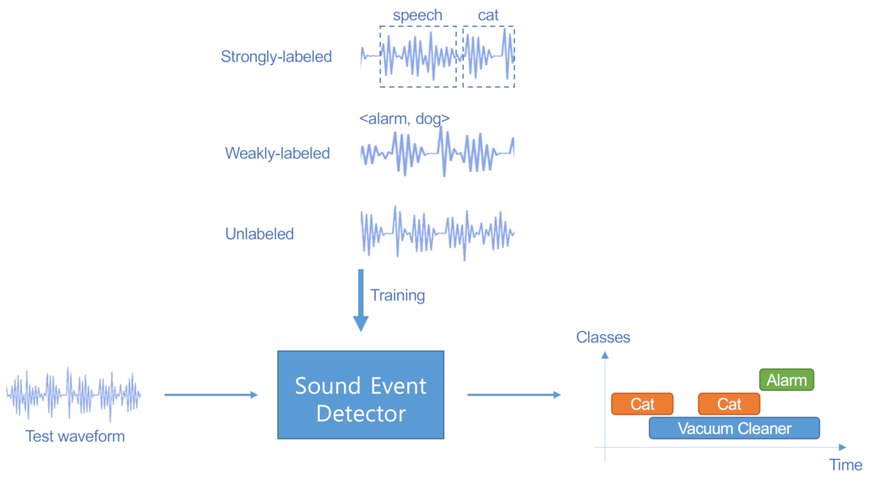
2.1. Problem Description

As mentioned in the Introduction, we aim to develop a data-dependent feature extraction method for weakly supervised domestic SED system. The target system and problem are designed in accordance with the Detection and Classification of Acoustic Scenes and Events (DCASE) 2020 Task 4 [34]. The target system aims to detect sound events with class, onset time, and offset time labels through a weakly-supervised training. In this training, some of the dataset annotations are omitted. More specifically, the dataset may be categorized into three types: strongly-labeled, weakly-labeled, and unlabeled data. The strongly-labeled data provide all the required information: sound class, onset time, and offset time annotations. The weakly-labeled data provide only part of the information, for example the sound class label only. The unlabeled data do not provide any information, only waveforms. A schematic diagram of the target system is presented in Figure 1.

Our goal is not to design the system itself but to develop a data-dependent feature extraction method for the system. Thus, we focus on the non-negative matrix decomposition technique, which is a sparse representation tool for acoustic signal data.

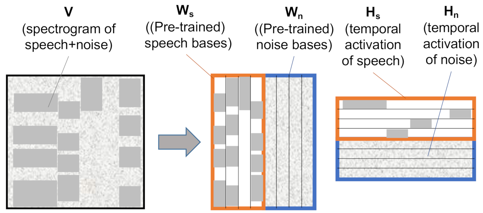
2.2. Non-Negative Matrix Factorization

The NMF method, which was developed by Lee and Seung [21,35], is employed to decompose a non-negative matrix $\mathbf{V}\in {\mathbb{R}}_{K\times N}^{+}$ into two matrices, $\mathbf{W}\in {\mathbb{R}}_{K\times R}^{+}$ and $\mathbf{H}\in {\mathbb{R}}_{R\times N}^{+}$, that satisfy the following relation [35]:

$$\mathbf{V}\approx \mathbf{WH}.$$

(1)

The matrices $\mathbf{W}$ and $\mathbf{H}$ can be estimated via alternating optimization of the two equations as [35,36]

$$\begin{array}{c}\hfill \mathbf{W}=arg\underset{\mathbf{W}}{min}D\left(\mathbf{V}|\mathbf{WH}\right)\mathrm{for} \mathrm{fixed}\mathbf{H},\end{array}$$

(2)

$$\begin{array}{c}\hfill \mathbf{H}=arg\underset{\mathbf{H}}{min}D\left(\mathbf{V}|\mathbf{WH}\right)\mathrm{for} \mathrm{fixed}\mathbf{W},\end{array}$$

(3)

where $D\left(\mathbf{V}|\mathbf{WH}\right)$ denotes the distance function between $\mathbf{V}$ and $\mathbf{WH}$. The distance functions can be optimized by the multiplicative update rule as [35]

$$\begin{array}{c}\hfill \mathbf{W}\leftarrow \mathbf{W}\otimes \frac{\left[\mathbf{V}/\left(\mathbf{WH}\right)\right]{\mathbf{H}}^T}{1_{K\times N}{\mathbf{H}}^T},\end{array}$$

(4)

$$\begin{array}{c}\hfill \mathbf{H}\leftarrow \mathbf{H}\otimes \frac{{\mathbf{W}}^T\left[\mathbf{V}/\left(\mathbf{WH}\right)\right]}{{\mathbf{W}}^T{\mathbf{1}}_{K\times N}},\end{array}$$

(5)

when the Kullback–Leibler divergence (KLD) is used as the distance function, where ${\mathbf{1}}_{K\times N}$ denotes a $K\times N$ matrix of ones, and

$$\begin{array}{c}\hfill \mathbf{W}\leftarrow \mathbf{W}\otimes \frac{{\mathbf{VH}}^T}{{\mathbf{WHH}}^T},\end{array}$$

(6)

$$\begin{array}{c}\hfill \mathbf{H}\leftarrow \mathbf{H}\otimes \frac{{\mathbf{W}}^T\mathbf{V}}{{\mathbf{W}}^T\mathbf{WH}},\end{array}$$

(7)

when the Euclidean distance is used, where ⊗ and the fraction denote the Hadamard (element-wise) product and division, respectively.

The NMF method has been widely employed in the recent acoustic signal processing studies to analyze a music signal into several musical notes or to reduce noise signals from the speech signals. Such interest can be attributed to the fact that the frequency basis matrix, $\mathbf{W}$, and the temporal basis matrix, $\mathbf{H}$, represent the frequency characteristics and temporal envelop of acoustic signal components, respectively. More specifically, speech denoizing methods divide the bases into two classes, speech and noise, and remove the noise bases after calculating the temporal bases of each class, as shown in Figure 2.

3. Proposed System

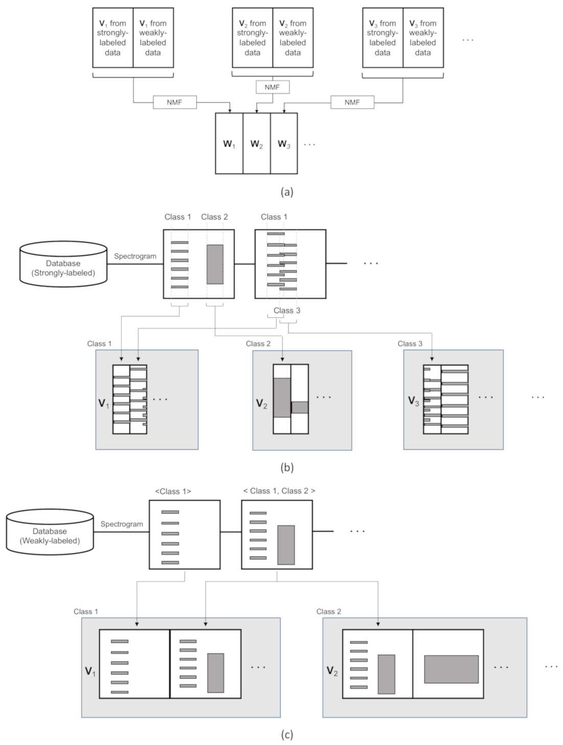
3.1. Strategy for the Frequency Basis Learning

Similar to the previous studies [5,31], the temporal basis matrix $\mathbf{H}$ is used as a feature. To extract the feature matrix, the frequency basis matrix needs to be estimated in advance. Inspired by speech denoizing [27] and reverberation suppression [37] techniques based on NMF [27], the frequency basis matrix of each class is independently estimated from the spectrogram set of the class, as presented in Figure 3a. In this method, the frequency basis matrix is divided into C groups as [31]

$$\mathbf{W}=\left[{\mathbf{W}}_1{\mathbf{W}}_2\cdots {\mathbf{W}}_C\right].$$

(8)

Each group denoted by ${\mathbf{W}}_c$ is a $K\times R_C$ matrix, where $R_C$ denotes the basis number of each class. The frequency and temporal basis matrices can be estimated by optimizing various cost functions. KLD is one of the common choices in the acoustic signal processing field. Therefore, the frequency and temporal basis matrices are iteratively updated by

$$\begin{array}{c}\hfill {\mathbf{W}}_c\leftarrow {\mathbf{W}}_c\otimes \frac{\left[{\mathbf{V}}_c/\left({\mathbf{W}}_c{\mathbf{H}}_c\right)\right]{\mathbf{H}}_c^T}{{\mathbf{1}}_{K\times N_c}{\mathbf{H}}_c^T}\end{array}$$

(9)

$$\begin{array}{c}\hfill {\mathbf{H}}_c\leftarrow {\mathbf{H}}_c\otimes \frac{{\mathbf{W}}_c^T\left[{\mathbf{V}}_c/\left({\mathbf{W}}_c{\mathbf{H}}_c\right)\right]}{{\mathbf{W}}_c^T{\mathbf{1}}_{K\times N_c}},\end{array}$$

(10)

which is similar to Equations (4) and (5), where ${\mathbf{V}}_c$ and ${\mathbf{H}}_c$ denote $K\times N_c$ data matrix and $R_C\times N_c$ temporal basis matrix, respectively, and $N_c$ stands for the total number of frames in the data matrix of the cth class.

Since weakly-supervised SED has a heterogeneous database, different learning strategies for each type of data need to be developed. In the case of strongly-labeled data, which contains the class and temporal information, the data matrix is a set of audio clips with a cut-off part, as presented in Figure 3b. As can be seen in the figure, there is a risk of data mixing from different classes. For example, if we assume that we want to generate the data matrix $\mathbf{V}$ for Class A, there may be various combinations, e.g., A–B, A–C, and A–D. However, even in this case, the data from Class A is expected to be dominant. Thus, the frequency matrix $\mathbf{W}$ can be expected to represent the characteristics of Class A if we choose a sufficiently small rank for matrix $\mathbf{W}$.

For the weakly-labeled data that do not contain an onset and offset information, the temporal information cannot be utilized. Therefore, we compose the data matrix $\mathbf{V}$ by just cascading the clips, as shown in Figure 3c. Unlike the case of the strongly-labeled data, where only parts of the event overlap, in the weakly-labeled data, waveforms from different classes are completely mixed when two or more classes are in one clip. Therefore, it is expected that the training of matrix $\mathbf{W}$ is more affected by the unwanted class interference problem compared to strongly-labeled data. Therefore, we evaluate the effect of the unwanted class interference problem on the weakly-labeled data.

3.2. Iterative and Non-Iterative Feature Extraction Methods

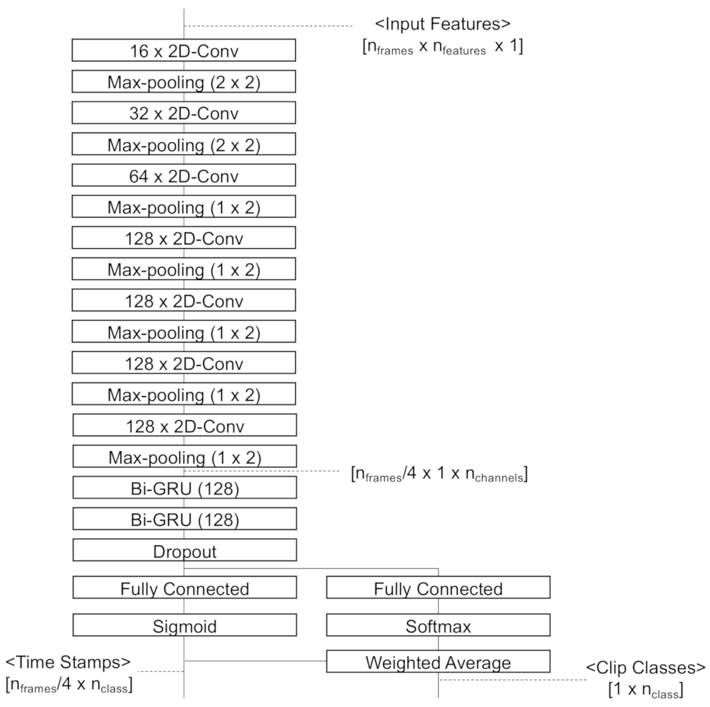
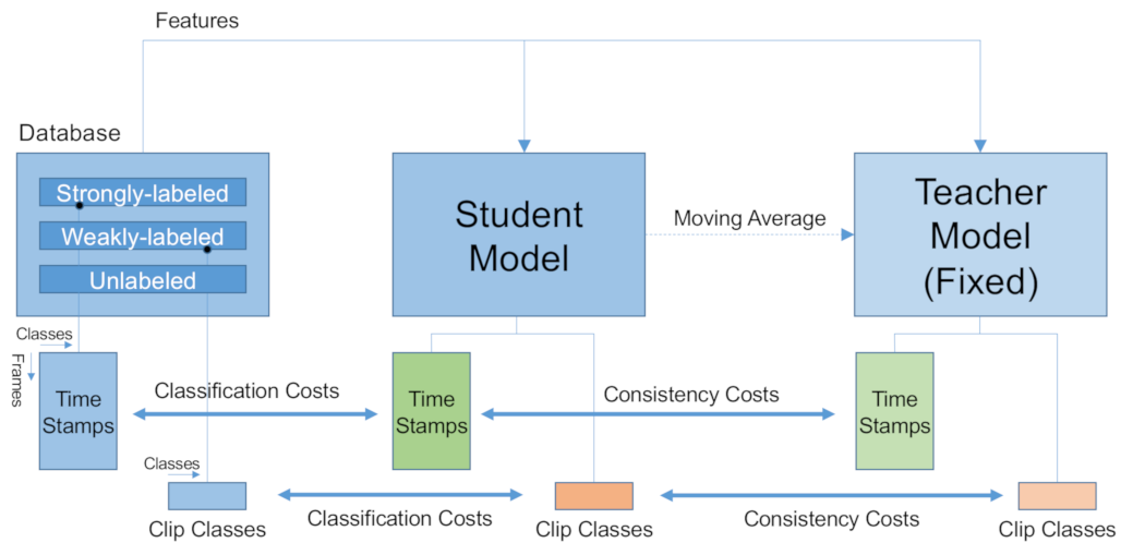
Once the frequency basis matrix $\mathbf{W}$ is trained, the feature matrix ${\mathbf{H}}_{clip}$ can be extracted from the data matrix ${\mathbf{V}}_{clip}$ of an audio clip via the iteration of [31]

$${\mathbf{H}}_{clip}\leftarrow {\mathbf{H}}_{clip}\otimes \frac{{\mathbf{W}}^T\left[{\mathbf{V}}_{clip}/\left(\mathbf{W}{\mathbf{H}}_{clip}\right)\right]}{{\mathbf{W}}^T{\mathbf{1}}_{K\times N_{clip}}}.$$

(11)

with minimization of the KLD (as Equation (5)).

In this paper, we also develop a non-iterative feature extraction method. To achieve this goal, we develop a closed-form solution for ${\mathbf{H}}_{clip}$ which makes the gradient of the divergence function with regard to ${\mathbf{H}}_{clip}$ zero (that is, ${\nabla }_{{\mathbf{H}}_{clip}}D\left({\mathbf{V}}_{clip}|{\mathbf{WH}}_{clip}\right)=0$). In addition, a solution with simple operations, e.g. matrix multiplication, is a preferred one because it is easy to implement.

The NMF-based methods for acoustic signal processing mainly use three types of distance functions: KLD, Euclidean distance, and Itakura–Saito divergence (ISD). The three distance functions are in the $\beta$-divergence family, which is expressed by [38]:

$$D_{\beta }\left(x|y\right)=\left\{\begin{array}{cc}\frac{x}{y}-log\frac{x}{y}-1\hfill & \beta =0\hfill \\ x\left(logx-logy\right)+\left(y-x\right)\hfill & \beta =1\hfill \\ \frac{1}{\beta \left(\beta -1\right)}\left(x^{\beta }+(\beta -1)y^{\beta }-\beta x{y}^{\beta -1}\right)\hfill & \mathrm{otherwise}\hfill \end{array}\right.$$

(12)

where x and y are arbitrary values and $\beta$ is a constant to adjust the cost function among the Euclidean ($\beta =2$), KLD ($\beta =1$), and ISD ($\beta =0$). In our problem, x and y are elements of the matrices ${\mathbf{V}}_{clip}$ and ${\mathbf{WH}}_{clip}$, respectively, and the gradient of the beta-divergence with regard to ${\mathbf{H}}_{clip}$ is [38]

$${\nabla }_{{\mathbf{H}}_{clip}}{D}_{\beta }\left({\mathbf{V}}_{clip}|{\mathbf{WH}}_{clip}\right)={\mathbf{W}}^T\left\{{\left({\mathbf{WH}}_{clip}\right)}^{.\left[\beta -2\right]}\otimes \left({\mathbf{WH}}_{clip}-{\mathbf{V}}_{clip}\right)\right\}$$

(13)

where ${\mathbf{A}}^{.\left[n\right]}$ denotes element-wise nth power of matrix $\mathbf{A}$. Because Equation (13) includes matrix multiplications, element-wise products and power, and the relationship between these operations is also complex. Therefore, it is not easy to find a solution that makes Equation (13) zero, and it is even more difficult to find a solution consisting of simple matrix multiplications. One easy way is to make the term of the left of the Hadamard product, ${\left(\mathbf{WH}\right)}^{.\left[\beta -2\right]}$, equal to one. In this case, $\beta$ becomes 2.0, and the divergence function becomes the Euclidean distance.

The Euclidean distance function can be defined using the Frobenius norm as

$$D_{EUC}\left({\mathbf{V}}_{clip}|{\mathbf{WH}}_{clip}\right)=\frac{1}{2}{∥{\mathbf{V}}_{clip}-{\mathbf{WH}}_{clip}∥}_F^2,$$

(14)

and the gradient of the cost function with respect to ${\mathbf{H}}_{clip}$ is

$${\nabla }_{{\mathbf{H}}_{clip}}{D}_{EUC}\left({\mathbf{V}}_{clip}|{\mathbf{WH}}_{clip}\right)=-{\mathbf{W}}^T\left[{\mathbf{V}}_{clip}-{\mathbf{WH}}_{clip}\right].$$

(15)

Since the cost function in Equation (14) is convex, the optimal solution of the cost function makes the gradient zero. Therefore, the optimal solution of ${\mathbf{H}}_{clip}$ needs to satisfy the relationship:

$${\mathbf{W}}^T{\mathbf{V}}_{clip}-{\mathbf{W}}^T{\mathbf{WH}}_{clip}=\mathbf{0}$$

(16)

and therefore

$$\begin{array}{cc}\hfill {\mathbf{H}}_{clip}& ={\left[{\mathbf{W}}^T\mathbf{W}\right]}^{-1}{\mathbf{W}}^T{\mathbf{V}}_{clip}\hfill \\ \hfill & ={\mathbf{W}}^{†}{\mathbf{V}}_{clip},\hfill \end{array}$$

(17)

where ${\mathbf{W}}^{†}$ denotes the Moore–Penrose pseudo-inverse of the matrix $\mathbf{W}$. Since the frequency basis matrix $\mathbf{W}$ is pre-trained and fixed, ${\mathbf{W}}^{†}$ is also defined a priori. Thus, feature extraction can be performed via a simple production using Equation (17).

The pseudo-inverse can be implemented via the singular value decomposition [39]. If we assume that the matrix $\mathbf{W}$ is decomposed as

$$\mathbf{W}=\mathbf{U}\mathbf{\Sigma }{\mathbf{V}}^H,$$

(18)

where $\mathbf{U}$ and $\mathbf{V}$ denote $K\times K$ and $R\times R$ matrices, respectively, and $\mathbf{\Sigma }$ denotes the $K\times R$ diagonal matrix whose elements are singular values of $\mathbf{W}$, then the pseudo-inverse ${\mathbf{W}}^{†}$ can be calculated as

$${\mathbf{W}}^{†}=\mathbf{V}{\mathbf{\Sigma }}^{†}{\mathbf{U}}^H,$$

(19)

where ${\Sigma }^{†}$ is a matrix formed from $\Sigma$ by taking the element-wise inverse of the non-zero elements and shaping the matrix as $R\times K$. In practice, the small singular values can be ignored as

$${\left[{\mathbf{\Sigma }}^{†}\right]}_{r,k}=\left\{\begin{array}{cc}1/{\left[\mathbf{\Sigma }\right]}_{k,r}\hfill & \mathrm{if}{\left[\mathbf{\Sigma }\right]}_{k,r}>\delta ,\hfill \\ 0\hfill & \mathrm{otherwise},\hfill \end{array}\right.$$

(20)

where ${\left[\mathbf{\Sigma }\right]}_{k,r}$ denotes the $\left(k,r\right)$th element of the matrix $\mathbf{\Sigma }$ and $\delta$ is an arbitrary threshold.

3.3. Classifier

To develop a feature extraction method and evaluate the performance of our method, a conventional convolutional recurrent neural network (CRNN) with a mean-teacher model is adopted [40,41,42]. Figure 4 presents the details of the network structure of the CRNN classifier. The convolutional layers and the corresponding max-pooling layers are designed so that the $n_{feature}$ axis of the output of the CNN layers is equal to unity. The RNN layers and the fully connected layer make the frame-wise probability of the classes, which is denoted by “Time Stamps” in Figure 4. To train the classifier using the weakly-labeled data, then it also generates the “Clip Class” output, which denotes the existing classes in a clip. The element of the clip class output $\mathbf{C}$ is calculated by weighted average as

$${\left[\mathbf{C}\right]}_c=\frac{{\sum }_{n=0}^{N_{out}-1}{\left[\mathbf{P}\right]}_{n,c}{\left[{\mathbf{P}}_{softmax}\right]}_{n,c}}{{\sum }_{n=0}^{N_{out}-1}{\left[{\mathbf{P}}_{softmax}\right]}_{n,c}},$$

(21)

where $N_{out}$ denotes the frame number of the classifier output of a sound clip.

The mean-teacher model is adopted to train the classifier using both the labeled and unlabeled data, similar to state-of-the-art weakly-supervised SED systems [40,41]. The network parameters of the student model, $\mathit{\theta }$, are optimized to minimize the cost function as

$$J_{total}\left(\mathit{\theta }\right)=J_{class}\left(\mathit{\theta }\right)+\beta J_{consist}\left(\mathit{\theta }\right),$$

(22)

where $J_{class}\left(\mathit{\theta }\right)$ and $J_{consist}\left(\mathit{\theta }\right)$ denote the classification cost and the consistency cost, respectively, as presented in Figure 5. $\beta$ is the weight for the consistency cost. The parameters of the teacher model, ${\mathit{\theta }}_{teacher}$, are fixed during the training procedure and updated at the end of the training batch as

$${\mathit{\theta }}_{teacher}\leftarrow \alpha {\mathit{\theta }}_{teacher}+(1-\alpha )\mathit{\theta }$$

(23)

where $\alpha$ denotes the exponential weighting factor of the moving average.

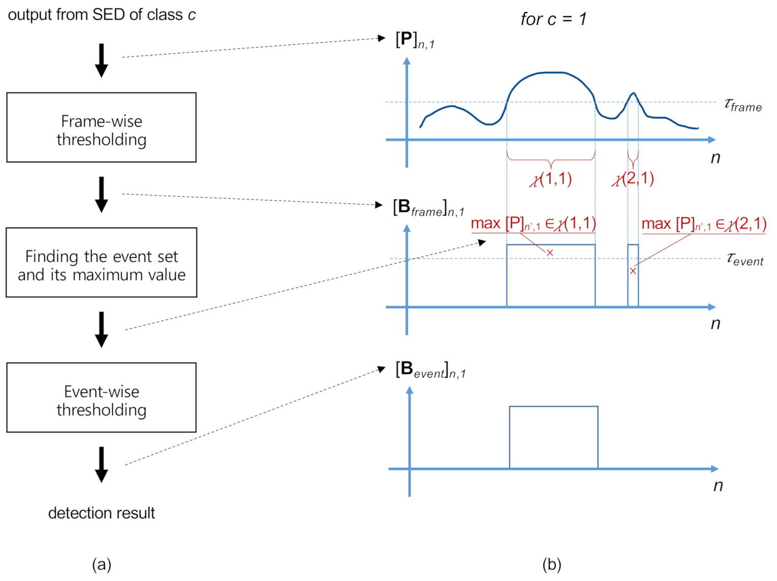
3.4. Post-Processing

The output of the sound event detector is a frame-wise probability of each class. Generally, the classifier output is post-processed with a certain threshold to determine whether the class is activated or not. The magnitude of the threshold value influences the classification performance. For example, a high threshold value can reduce false-positive errors but sometimes underestimates the length of the event, and vice versa. In this paper, the classifier output is first processed with a frame-wise threshold and then with an event-wise threshold to eliminate false-positive errors. The threshold value of the event-wise post-processing is set to be larger than that of the frame-wise post-processing.

When we refer to the classifier output as a matrix $\mathbf{P}$ of $N_{out}\times C$, the frame-wise binary matrix ${\mathbf{B}}_{frame}$ is calculated as

$${\left[{\mathbf{B}}_{frame}\right]}_{n,c}=\left\{\begin{array}{cc}1\hfill & \mathrm{if}{\left[\mathbf{P}\right]}_{n,c}\ge {\tau }_{frame},\hfill \\ 0\hfill & \mathrm{if}{\left[\mathbf{P}\right]}_{n,c}<{\tau }_{frame},\hfill \end{array}\right.$$

(24)

where C denotes the number of classes and ${\tau }_{frame}$ is the threshold for the frame-wise post-processing. Let us define $\chi (i,c)$ as the ith event set of class c as

$$\chi (i,c)=\left\{(n,c)|n_{onset}(i,c)\le n\le n_{offset}(i,c)\right\},$$

(25)

where $n_{onset}(i,c)$ and $n_{offset}(i,c)$ are the frame numbers of the ith onset and offset of class c, respectively. The result of the event-wise thresholding, ${\mathbf{B}}_{event}$, is obtained as

$${\left[{\mathbf{B}}_{event}\right]}_{n,c}=\left\{\begin{array}{cc}1\hfill & \mathrm{if}\left(\underset{(n^{\prime },c)\in {\chi }^{\prime }}{max}{\left[\mathbf{P}\right]}_{n^{\prime },c}\right)\ge {\tau }_{event}\hfill \\ 0\hfill & \mathrm{otherwise}\hfill \end{array}\right.,$$

(26)

where $(n^{\prime },c)\in {\chi }^{\prime }$ means that $(n^{\prime },c)$ belongs to ${\chi }^{\prime }$, and ${\chi }^{\prime }$ denotes a certain event set that contains $(n,c)$ as an element. Figure 6 presents a flow chart and an illustrative example of the proposed event-wise post-processing.

4. Evaluation

4.1. Evaluation Settings

To evaluate the proposed system for domestic SED, numerical simulations were performed using the DESED dataset of the DCASE 2020 Task 4 database, which is an audio dataset for weakly supervised sound event detection in domestic environments. The database consists of real-recorded subsets of Audioset [43] and Freesound [44]. Some of the data are synthesized using the SINS database [45] as background sounds.

There are 10 event classes: speech, dog, cat, alarm bell, dishes, frying, blender, running water, vacuum cleaner, and electric shaver. Each audio clip is a 10-s wav file with 44.1 (for the weakly-labeled and unlabeled data) or 16 kHz (for strongly-labeled data) sampling frequency. All audio files were resampled to a 16 kHz sampling frequency. The database consists of strongly-labeled data (2045 files, with event classes and time stamp information), weakly-labeled data (1578 files, with event classes information only), and unlabeled data (14412 files, without any annotation). The detailed information of the database configuration can be found in [34].

The audio clips were short-time-Fourier-transformed by a 1024-sample Hanning window with 75% overlap to match the number of input frames in the classifier for the baseline of the DCASE 2020 Task 4 [40]. To train the NMF frequency basis matrix, 200 iterations were performed to calculate both ${\mathbf{W}}_c$ and ${\mathbf{H}}_c$ matrices (Equations (9) and (10)) for each class. The number of the basis for each class was set to 13 (11 for the “vacuum cleaner” class) so that the dimension of the extracted feature was 128. In the case of iterative feature extraction, 50 iterations were performed for each clip to calculate ${\mathbf{H}}_{clip}$ (Equation (11)). The singular value threshold ($\delta$ in Equation (20)) was set to be a proportional to the maximum singular value as

$$\delta =\gamma \underset{k,r}{max}{\left[\mathbf{\Sigma }\right]}_{k,r},$$

(27)

where $\gamma$ denotes a proportionality constant.

The classifier was trained using Adam optimizer, and the learning rate was exponentially ramped up during 50 epochs to the maximum learning rate of 0.001. The classification and the consistency costs were categorical cross-entropy and mean-squared error, respectively, and the weight for the consistency costs, $\beta$, was set to 2.0. The classifier was trained using the training dataset of the DCASE database for 200 epochs and evaluated using the validation dataset. The batch size was set to 24, and the moving-average weighting factor, $\alpha$, of the mean-teacher model was 0.999.

The performances of the two types of post-processing systems, with and without the event-wise post-processing, were evaluated. The post-processing system without the event-wise post-processing consisted of only the frame-wise thresholding, and the threshold value was set to 0.5. The system with the event-wise post-processing consisted of the frame-wise and event-wise thresholding. The event threshold value was set to 0.8 as it exhibited good overall performance, while the frame thresholds were set to the optimal values that exhibited the best performance among $\left\{0.1,0.2,0.3,0.4,0.5,0.6,0.7\right\}$ for each class.

In this evaluation, the event-based F1-score was utilized as the performance measure, which is defined by a geometric mean of precision P and recall R as

$$F_1=\frac{2PR}{P+R},$$

(28)

where precision and recall are defined as

$$P=\frac{n_{TP}}{n_{TP}+n_{FP}},$$

(29)

and

$$R=\frac{n_{TP}}{n_{TP}+n_{FN}},$$

(30)

where $n_{FP}$, $n_{FN}$, and $n_{TP}$ denote the numbers of false answers (false positives), missing answers (false negatives), and correct answers (true positives). The answers were considered as “correct answer” if the onset error was smaller than 0.2 s, and the offset error was smaller than 0.2 s (or 20 % of the event duration). The criteria to determine the correct answers were set to be consistent with the baseline of the DCASE 2020 Task 4 [34]. Moreover, the performance of each class was micro-averaged, which aggregated the contributions of all the test samples regardless of the class, and macro-averaged, which averages the individual performance of each class.

4.2. Comparison of Various Features

Table 1. Averaged results of various features. The performance of the Cornell system was provided as a reference of comparison. The boldface means the best performance of each measure.

	w/o Event-Wise Post-Processing		w/ Event-Wise Post-Processing
	F1-Score [%] (Micro)	F1-Score [%] (Macro)	F1-Score [%] (Micro)	F1-Score [%] (Macro)
NMF(iterative)	35.06	31.58	40.12	39.23
NMF (non-iterative)	34.87	30.16	40.02	38.45
MelSpec	34.41	32.31	40.41	39.72
Log-Mel	30.27	29.88	35.11	36.60
GAM	32.15	33.09	37.23	39.81
CQT	32.25	28.76	37.28	35.36
Cornell et al. [46]	-	-	(with own post-processing)
			42.48	39.56

compares the proposed and conventional features that are commonly used in ASC and SED applications. The abbreviations MelSpec, Log-Mel, GAM, and CQT denote the Mel-spectrogram, log-Mel spectrum, gammatonegram, and constant-Q transform (CQT), respectively. The frequency basis matrix used to extract the NMF features in Table 1 was trained using strongly-labeled data only as it exhibited good overall performance. The effect of the data on the frequency basis training will be considered in the next subsection. The dimensions of the extracted features were all set to 128, similar to that in the Delphin–Poulet system [40], to compare the performances of the features without changing the structure of the classifier. The CQT was performed under 16 bins per octave and 32.7 Hz lower bound frequency. In total, 128 CQT bins (=8 octaves) corresponded to a frequency range of less than approximately 8 kHz. The proposed system was also compared with the Cornell system [46] including the log-Mel features with data augmentation, per-channel energy normalization (PCEN), mean-teacher CRNN, and post-processing with hidden Markov model (HMM), which was submitted to DCASE 2020 Task 4. The details of the sub-systems can be found in [46]. The training parameters (e.g., the weight for the consistency costs, number of epochs, batch size, and the moving-average weighting factor of the mean-teacher model) were set to the same values of the proposed system. Because the Cornell system has its own post-processing consisting of HMM and random forest optimization, the proposed event-wise post-processing was not applied to the Cornell system.

The performances of the NMF methods are comparable to those of the Mel-spectrogram and gammatonegram, the best among the conventional features, and are better than those of the log-Mel spectrum and CQT in all the performance measures. The comparison between the micro-averaged performance of the NMF and that of the Mel-spectrogram revealed that the NMF methods exhibited slightly better performances without the event-wise post-processing and slightly worse performances with the event-wise post-processing. The gammatonegram had the best performance in the macro-averaged F1-score among the features but demonstrated low performance in the micro-averaged F1-score. Moreover, the features extracted using the iterative and non-iterative NMF methods exhibited similar performances. Thus, the non-iterative NMF method can be considered as an alternative to the iterative NMF method. The micro-averaged and macro-averaged F1-scores of the proposed system are similar to and slightly less than that of the Cornell system, respectively. We think that the difference of the performance was caused by additional sub-systems in the Cornell system, such as PCEN, data augmentation, and random forest optimization of HMM post-processing.

Table 2. Class-wise F1-scores [%] of various features. The boldface means the best performance of each class.

	Electric Shaver	Speech	Dishes	Cat	Running Water	Dog	Frying	Blender	Alarm Bell	Vacuum Cleaner
ine NMF (iterative)	32.9	46.8	18.0	39.7	22.4	21.5	28.9	27.5	36.3	41.7
ine NMF (non-iterative)	24.1	43.9	21.9	39.5	25.7	22.1	22.8	22.1	39.6	39.9
ine MelSpec	35.7	45.0	18.0	39.1	30.9	17.4	24.0	32.0	32.0	49.0
ine Log-Mel	38.3	37.3	14.2	36.7	27.4	13.7	23.5	23.0	35.8	49.0
ine GAM	29.5	34.2	24.6	41.7	28.3	19.7	31.4	33.9	39.4	48.2
ine CQT	34.6	46.7	18.4	35.9	21.7	16.5	9.1	24.8	24.1	55.6

presents the class-wise F1-score performances. The gray background denotes the class where the NMF method exhibits better performance than that in the Mel-spectrogram, and the bold-face number stands for the best performance in each class. A scan be seen in the table, the NMF methods are advantageous for classes with harmonic structures (speech, dog, cat, and alarm bell) and disadvantageous for noise-like classes (electric shaver, blender, running water, and vacuum cleaner). The class-wise performances of the iterative and non-iterative NMFs are different. The iterative NMF has better performances for five classes (electric shaver, speech, frying, blender, and vacuum cleaner), similar performances for two classes (cat and dog), and worse performances for three classes (dishes, running water, and alarm bell). The last three classes (dishes, running water, and alarm bell) contained several impulsive sounds. Thus, the non-iterative method appeared to be useful for the impulsive sounds. However, we cannot easily come to this conclusion, as the frying sounds also contain impulsive ones.

2

There are two main differences between the iterative and non-iterative NMFs: divergence function and optimization method. The iterative NMF uses KLD and multiplicative update, and the non-iterative NMF employs Euclidean and closed-form solution. To analyze the effect on the class-wise performance, we compare the performances of the NMFs with an iterative NMF with Euclidean (for convenience, we call it NMF-EUC here). The iterative NMF and NMF-EUC have the same parameters and settings except for the divergence function. Figure 7 shows the comparison results. The iterative NMF is superior to the NMF-EUC in the classes of electric shaver, speech, frying, and blender, where the iterative NMF is superior to the non-iterative NMF. In other words, the tendencies in performances are similar for the NMF-EUC and non-iterative NMF. However, the difference in the performance of non-iterative NMF compared to iterative NMF is greater than that of NMF-EUC and iterative NMF. Therefore, it seems that the difference in the optimization method had a greater effect on the performance than that in the divergence function in this experiment.

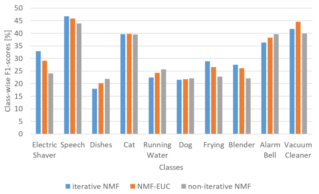
4.3. Effect of the Training Data on the Frequency Basis Learning

To analyze the effect of the training data on the frequency basis matrices in the NMF methods, the performances of the NMF methods were compared with the different frequency basis matrices from various parts of the database.

Table 3. Comparison results with different frequency basis matrices from various parts of the database.

	NMF (Iterative)		NMF (Non-Iterative)
	F1-Score [%] (Micro)	F1-Score [%] (Macro)	F1-Score [%] (Micro)	F1-Score [%] (Macro)
STR	40.12	39.23	40.02	38.45
WEAK(U)	40.02	38.89	38.98	37.65
WEAK	41.53	38.28	39.01	37.76
STR + WEAK(U)	38.91	37.50	38.39	38.79
STR + WEAK	38.51	37.39	39.97	38.40

presents the F1-score results of different frequency basis matrices with the event-wise post-processing. STR, WEAK, and WEAK(U) denote the frequency basis matrices trained by the strongly-labeled data, weakly-labeled data, and weakly-labeled unitary label data, which consist of single-class clips, respectively.

As presented in Table 3, the strongly-labeled data exhibited relatively good overall performance. The weakly-labeled data demonstrated good micro-averaged performance for iterative NMF but degraded performances for the other criteria, including non-iterative NMF. Using both the strongly- and weakly-labeled unitary label data (STR + WEAK(U)) also had good macro-averaged performance for non-iterative NMF, but it also showed degraded performances for other criteria. Conversely, the performance of the weakly-labeled unitary label data (WEAK(U)) did not exceed that of the weakly-labeled data (WEAK) that has interference classes. For instance, Class 2 data interferes with the training of Class 1 frequency basis matrix (Figure 3c). Therefore, we suggest that the class interference problem does not significantly affect the classification performance.

4.4. Thresholding Singular Values for Calculating the Pseudo-Inverse Matrix

To extract the proposed feature instantaneously, the Moore–Penrose pseudo-inverse of the frequency basis matrix needs to be calculated in advance using Equation (17). As follows from Equations (19) and (20), the pseudo-inverse matrix can be calculated via singular value decomposition with thresholding of the small singular values. The threshold, which is one of the design parameters, is related to stability and sparsity of the pseudo-inverse matrix. Thus, it may affect the performance of the extracted features. Therefore, we evaluated the effect of the threshold on the classification performance.

Table 4. Comparison results with various thresholds of singular values for calculating the pseudo-inverse.

	w/o Event-Wise Post-Processing		w/ Event-Wise Post-Processing
	F1-Score [%] (Micro)	F1-Score [%] (Macro)	F1-Score [%] (Micro)	F1-Score [%] (Macro)
$\gamma =0.001$	27.26	24.56	35.16	34.24
$\gamma =0.005$	33.59	29.95	39.59	37.94
$\gamma =0.01$	34.87	30.16	40.02	38.45
$\gamma =0.05$	32.52	28.35	38.51	36.23
$\gamma =0.1$	21.45	10.88	26.45	17.39

presents the classification performances with various threshold values. As follows from Equation (27), $\delta$ denotes the ratio of the threshold value to the maximum singular value. Among the test values, $\gamma =0.01$ exhibits the best performance, while $\gamma =0.005$ and $\gamma =0.05$ exhibit comparable performances. However, $\gamma =0.001$ and $\gamma =0.1$ result in significantly degraded performances. Therefore, $\gamma$ values between 0.005 and 0.05 are good choices for our system.

5. Conclusions

In this paper, two NMF-based feature extraction methods are proposed for weakly supervised SED. Inspired by the NMF applications in the acoustic signal processing systems capable of analyzing the frequency characteristics of the acoustic signals, the proposed methods were designed to extract features from heterogeneous database for weakly supervised SED. To generate the frequency basis matrix, the class-wise data matrices were composed from strongly- and weakly-annotated data. The class-wise frequency basis matrices were estimated using the NMF algorithm with the KLD, and then cascaded to compose the whole frequency basis matrix. In the iterative feature extraction method, the temporal basis matrix was calculated via iterations of the NMF equations using the whole frequency basis matrix. Moreover, we developed a non-iterative feature extraction method using a least-squares solution of the NMF problem. The classifier was constructed based on the mean-teacher model for the proposed features and enhanced by the proposed event-wise post-processing method.

To evaluate the proposed data-dependent feature extraction methods, simulations of weakly supervised SED were performed using the DCASE 2020 Task 4 database. The proposed methods were compared with the conventional features, e.g., Mel-spectrogram, log-Mel spectrum, gammatonegram, and CQT. Although the proposed features did not outperform other features, they yielded results comparable to those of the Mel-spectrogram and gammatonegram, which are state-of-the-art features. Moreover, they demonstrated 3–5% better F1-score performance than the log-Mel-spectrum and CQT.

References

1. Chu, S.; Narayanan, S.; Kuo, C.C.J.; Mataric, M.J. Where am I? Scene recognition for mobile robots using audio features. In Proceedings of the 2006 IEEE International Conference on Multimedia and Expo, Toronto, Canada, 9–12 July 2006; pp. 885–888. [Google Scholar]
2. Ellis, D.P.; Lee, K. Minimal-impact audio-based personal archives. In Proceedings of the the 1st ACM Workshop on Continuous Archival and Retrieval of Personal Experiences, New York, NY, USA, 15 October 2004; pp. 39–47. [Google Scholar]
3. Barchiesi, D.; Giannoulis, D.; Stowell, D.; Plumbley, M.D. Acoustic scene classification: Classifying environments from the sounds they produce. IEEE Signal Process. Mag. 2015, 32, 16–34. [Google Scholar] [CrossRef]
4. Mesaros, A.; Heittola, T.; Virtanen, T. A multi-device dataset for urban acoustic scene classification. In Proceedings of the Detection and Classification of Acoustic Scenes and Events 2018 Workshop (DCASE2018), Surrey, UK, 19–20 November 2018; pp. 9–13. [Google Scholar]
5. Bisot, V.; Serizel, R.; Essid, S.; Richard, G. Feature learning with matrix factorization applied to acoustic scene classification. IEEE/ACM Trans. Audio Speech Lang. Process. 2017, 25, 1216–1229. [Google Scholar] [CrossRef] [Green Version]
6. Cakır, E.; Parascandolo, G.; Heittola, T.; Huttunen, H.; Virtanen, T. Convolutional recurrent neural networks for polyphonic sound event detection. IEEE/ACM Trans. Audio Speech Lang. Process. 2017, 25, 1291–1303. [Google Scholar] [CrossRef] [Green Version]
7. Huang, Z.; Jiang, D. Acoustic Scene Classification Based on Deep Convolutional Neuralnetwork with Spatial-Temporal Attention Pooling; Technical Report; DCASE2019 Challenge; DCASE Community: Washington, DC, USA, 2019. [Google Scholar]
8. Liu, H.; Wang, F.; Liu, X.; Guo, D. An Ensemble System for Domestic Activity Recognition; Technical Report; DCASE2018 Challenge; DCASE Community: Washington, DC, USA, 2018. [Google Scholar]
9. Chen, H.; Liu, Z.; Liu, Z.; Zhang, P.; Yan, Y. Integrating the Data Augmentation Scheme with Various Classifiers for Acoustic Scene Modeling; Technical Report; DCASE2019 Challenge; DCASE Community: Washington, DC, USA, 2019. [Google Scholar]
10. Inoue, T.; Vinayavekhin, P.; Wang, S.; Wood, D.; Greco, N.; Tachibana, R. Domestic Activities Classification Based on CNN Using Shuffling and Mixing Data Augmentation; Technical Report; DCASE2018 Challenge; DCASE Community: Washington, DC, USA, 2018. [Google Scholar]
11. Valenti, M.; Squartini, S.; Diment, A.; Parascandolo, G.; Virtanen, T. A convolutional neural network approach for acoustic scene classification. In Proceedings of the 2017 International Joint Conference on Neural Networks (IJCNN), Anchorage, AK, USA, 14–19 May 2017; pp. 1547–1554. [Google Scholar]
12. Moore, B.C. An Introduction to the Psychology of Hearing; Brill Academy Press: Leiden, The Netherlands, 2012. [Google Scholar]
13. Bisot, V.; Essid, S.; Richard, G. HOG and subband power distribution image features for acoustic scene classification. In Proceedings of the 2015 23rd European Signal Processing Conference (EUSIPCO), Nice, France, 31 August–4 September 2015; pp. 719–723. [Google Scholar]
14. Roma, G.; Nogueira, W.; Herrera, P.; De Boronat, R. Recurrence quantification analysis features for auditory scene classification. IEEE Aasp Chall. Detect. Classif. Acoust. Scenes Events 2013. [Google Scholar] [CrossRef]
15. Gowdy, J.N.; Tufekci, Z. Mel-scaled discrete wavelet coefficients for speech recognition. In Proceedings of the 2000 IEEE International Conference on Acoustics, Speech, and Signal Processing, (Cat. No. 00CH37100), Istanbul, Turkey, 5–9 June 2000; Volume 3, pp. 1351–1354. [Google Scholar]
16. Waldekar, S.; Saha, G. Wavelet Transform Based Mel-scaled Features for Acoustic Scene Classification. In Proceedings of the Interspeech 2018, Hyderabad, India, 2–6 September 2018; pp. 3323–3327. [Google Scholar]
17. Waldekar, S.; Kumar A, K.; Saha, G. Mel-Scaled Wavelet-Based Features for Sub-Task A and Texture Features for Sub-Task B of DCASE 2020 Task 1; Technical Report; DCASE2020 Challenge; DCASE Community: Washington, DC, USA, 2020. [Google Scholar]
18. Phan, H.; Koch, P.; Katzberg, F.; Maass, M.; Mazur, R.; Mertins, A. Audio scene classification with deep recurrent neural networks. arXiv 2017, arXiv:1703.04770. [Google Scholar]
19. Valero, X.; Alias, F. Gammatone cepstral coefficients: Biologically inspired features for non-speech audio classification. IEEE Trans. Multimed. 2012, 14, 1684–1689. [Google Scholar] [CrossRef]
20. Abdi, H.; Williams, L.J. Principal component analysis. Wiley Interdiscip. Rev. Comput. Stat. 2010, 2, 433–459. [Google Scholar] [CrossRef]
21. Lee, D.D.; Seung, H.S. Learning the parts of objects by non-negative matrix factorization. Nature 1999, 401, 788–791. [Google Scholar] [CrossRef] [PubMed]
22. Smaragdis, P.; Brown, J.C. Non-negative matrix factorization for polyphonic music transcription. In Proceedings of the 2003 IEEE Workshop on Applications of Signal Processing to Audio and Acoustics, New Paltz, NY, USA, 19–22 October 2003; pp. 177–180. [Google Scholar]
23. Bertin, N.; Badeau, R.; Vincent, E. Enforcing harmonicity and smoothness in Bayesian non-negative matrix factorization applied to polyphonic music transcription. IEEE Trans. Audio Speech Lang. Process. 2010, 18, 538–549. [Google Scholar] [CrossRef]
24. Benetos, E.; Dixon, S.; Giannoulis, D.; Kirchhoff, H.; Klapuri, A. Automatic music transcription: Challenges and future directions. J. Intell. Inf. Syst. 2013, 41, 407–434. [Google Scholar] [CrossRef] [Green Version]
25. Wilson, K.W.; Raj, B.; Smaragdis, P.; Divakaran, A. Speech denoising using nonnegative matrix factorization with priors. In Proceedings of the 2008 IEEE International Conference on Acoustics, Speech and Signal Processing, Las Vegas, NV, USA, 30 March–4 April 2008; pp. 4029–4032. [Google Scholar]
26. Kwon, K.; Shin, J.W.; Kim, N.S. NMF-based speech enhancement using bases update. IEEE Signal Process. Lett. 2014, 22, 450–454. [Google Scholar] [CrossRef]
27. Fan, H.T.; Hung, J.w.; Lu, X.; Wang, S.S.; Tsao, Y. Speech enhancement using segmental nonnegative matrix factorization. In Proceedings of the 2014 IEEE International Conference on Acoustics, Speech and Signal Processing (ICASSP), Florence, Italy, 4–9 May 2014; pp. 4483–4487. [Google Scholar]
28. Cauchi, B. Non-Negative Matrix Factorisation Applied to Auditory Scenes Classification. Master’s Thesis, Master ATIAM, Université Pierre et Marie Curie, Paris, France, 2011. [Google Scholar]
29. Bisot, V.; Serizel, R.; Essid, S.; Richard, G. Acoustic scene classification with matrix factorization for unsupervised feature learning. In Proceedings of the 2016 IEEE International Conference on Acoustics, Speech and Signal Processing (ICASSP), Shanghai, China, 20–25 March 2016; pp. 6445–6449. [Google Scholar]
30. Liu, D.C.; Nocedal, J. On the limited memory BFGS method for large scale optimization. Math. Program. 1989, 45, 503–528. [Google Scholar] [CrossRef] [Green Version]
31. Lee, S.; Pang, H.S. Feature Extraction Based on the Non-Negative Matrix Factorization of Convolutional Neural Networks for Monitoring Domestic Activity With Acoustic Signals. IEEE Access 2020, 8, 122384–122395. [Google Scholar] [CrossRef]
32. Choi, K.; Joo, D.; Kim, J. Kapre: On-gpu audio preprocessing layers for a quick implementation of deep neural network models with keras. arXiv 2017, arXiv:1706.05781. [Google Scholar]
33. Cheuk, K.W.; Anderson, H.; Agres, K.; Herremans, D. nnAudio: An on-the-Fly GPU Audio to Spectrogram Conversion Toolbox Using 1D Convolutional Neural Networks. IEEE Access 2020, 8, 161981–162003. [Google Scholar] [CrossRef]
34. Turpault, N.; Serizel, R.; Parag Shah, A.; Salamon, J. Sound event detection in domestic environments with weakly labeled data and soundscape synthesis. In Proceedings of the Detection and Classification of Acoustic Scenes and Events 2019 Workshop, New York, NY, USA, 25–26 October 2019. [Google Scholar]
35. Lee, D.D.; Seung, H.S. Algorithms for non-negative matrix factorization. In Advances in Neural Information Processing Systems; MIT Press: Cambridge, MA, USA, 2001; pp. 556–562. [Google Scholar]
36. Cichocki, A.; Zdunek, R.; Phan, A.H.; Amari, S.I. Nonnegative Matrix and Tensor Factorizations: Applications to Exploratory Multi-Way Data Analysis and Blind Source Separation; John Wiley & Sons: Hoboken, NJ, USA, 2009. [Google Scholar]
37. Lee, S.; Lim, J.S. Reverberation suppression using non-negative matrix factorization to detect low-Doppler target with continuous wave active sonar. EURASIP J. Adv. Signal Process. 2019, 2019, 11. [Google Scholar] [CrossRef]
38. Févotte, C.; Bertin, N.; Durrieu, J.L. Nonnegative matrix factorization with the Itakura-Saito divergence: With application to music analysis. Neural Comput. 2009, 21, 793–830. [Google Scholar] [CrossRef] [PubMed]
39. Ben-Israel, A.; Greville, T.N. Generalized Inverses: Theory and Applications; Springer Science & Business Media: Berlin/Heidelberg, Germany, 2003; Volume 15. [Google Scholar]
40. Delphin-Poulat, L.; Plapous, C. Mean Teacher with Data Augmentation for Dcase 2019 Task 4; Technical Report; Orange Labs: Lannion, France, 2019. [Google Scholar]
41. Jiakai, L. Mean Teacher Convolution System for Dcase 2018 Task 4; Technical Report; DCASE2018 Challenge; DCASE Community: Washington, DC, USA, 2018. [Google Scholar]
42. Tarvainen, A.; Valpola, H. Mean teachers are better role models: Weight-averaged consistency targets improve semi-supervised deep learning results. arXiv 2017, arXiv:1703.01780. [Google Scholar]
43. Gemmeke, J.F.; Ellis, D.P.W.; Freedman, D.; Jansen, A.; Lawrence, W.; Moore, R.C.; Plakal, M.; Ritter, M. Audio Set: An ontology and human-labeled dataset for audio events. Proc. IEEE ICASSP 2017. [Google Scholar] [CrossRef]
44. Fonseca, E.; Pons, J.; Favory, X.; Font, F.; Bogdanov, D.; Ferraro, A.; Oramas, S.; Porter, A.; Serra, X. Freesound Datasets: A platform for the creation of open audio datasets. In Proceedings of the 18th International Society for Music Information Retrieval Conference (ISMIR 2017), Suzhou, China, 23–27 October 2017; pp. 486–493. [Google Scholar]
45. Dekkers, G.; Lauwereins, S.; Thoen, B.; Adhana, M.W.; Brouckxon, H.; Van Waterschoot, T.; Vanrumste, B.; Verhelst, M.; Karsmakers, P. The SINS Database for Detection of Daily Activities in a Home Environment Using an Acoustic Sensor Network. In Proceedings of the Detection and Classification of Acoustic Scenes and Events 2017 Workshop (DCASE2017), Munich, Germany, 16–17 November 2017; pp. 32–36. [Google Scholar]
46. Cornell, S.C.; Pepe, G.; Principi, E.; Pariente, M.; Olvera, M.; Gabrielli, L.; Squartini, S. The UNIVPM-INRIA Systems for The DCASE 2020 Task 4; Technical Report; DCASE2020 Challenge; DCASE Community: Washington, DC, USA, 2020. [Google Scholar]
Figure 1. Problem description.
Applsci 11 01040 g001
Figure 2. Schematic diagram of the applications of the non-negative matrix factorization (NMF) methods to the acoustic signal processing systems.
Applsci 11 01040 g002
Figure 3. Block diagrams for: (a) the learning of the frequency basis; (b) the learning of the composition of the data matrix from strongly-labeled data; and (c) the learning of the composition of the data matrix from weakly-labeled data.
Applsci 11 01040 g003
Figure 4. Block diagram of the network structure for the CRNN classifier.
Applsci 11 01040 g004
Figure 5. Block diagram of the mean-teacher model.
Applsci 11 01040 g005
Figure 6. (a) A flow chart; and (b) an illustrative example of the event-wise post-processing.
Applsci 11 01040 g006
Figure 7. Performance comparison between the iterative NMF, NMF-EUC, and non-iterative NMF.
Applsci 11 01040 g007