Abstract
A novel differential method based on linear fitting is proposed to improve the accuracy of the pulse-ranging system. In this method, the Peak Points (PPs) of the traditional echo signal transformed into the Positive-Going Zero-Crossing Points (PGZCPs) of the differential echo signal. Then, we obtained the true zero-crossing point by the linear fitting of points near PGZCPs. We compared the differential method based on linear fitting (DMLF) and peak method. The Root Mean Square Error (RMSE) found with our method (0.1661 ns) is nearly a 50% reduction compared to that of the peak method (0.3318 ns), and a large number of experiments have demonstrated that the Relative Error (RE) of our proposed method is less than 30 ppm.
1. Introduction
Light detection and ranging (LiDAR) is a high-precision active ranging technology [1,2]. Due to the advantages of a large field of view, high resolution, and long-distance measurement, it has received much attention in recent years and has been widely used in target detection and recognition, environmental pollution perception, estimating ground topography, and autonomous vehicles [3,4,5,6,7,8]. To our knowledge, the system emits short laser pulses to illuminate the target, avalanche photodiode (APD) obtains the laser pulses reflected from the target’s surface, and then the time of flight (TOF) can figure out through subsequent digital processing equipment [9,10]. Therefore, the distance from the emitted source to targets can be calculated from the TOF [11]. The key to acquiring TOF is discriminating the exact arrival time of the echo pulse. Unfortunately, the timing accuracy is susceptible to interference from system error or surrounding noise. Some methods have already been proposed to improve the timing accuracy of TOF [12,13]. A leading-edge discriminator (LED) is a simple method, and the leading edge of the received pulse is detected as the signal crosses a certain threshold. However, the shortcoming of LED is that the timing moment will shift with the changes in amplitude in the echo signal. Therefore, there will likely be a few nanoseconds of walk error [14,15]. In order to decrease the walk error, some people use a peak discriminator (PD) to determine the timing moment, but the disadvantage of PD is that the Peak Points (PPs) are easily affected by both background noise and broadening echo pulse. These result in poor performance in the condition of low signal to noise rate (SNR) [16,17]. Yang, J, Zhao, W, et al. proposed a laser differential focal-length measurement method, which proves that the differential method can decrease the power of noise (including background noise, shot noise, thermal noise, and other random noise [18,19]) dramatically and has strong anti-interference capabilities [20,21].
This study aims to develop a technique for suppressing the surrounding noise and improving the performance of the pulse-ranging LiDAR. For this purpose, a novel differential method based on linear fitting (DMLF) is proposed. With this method, the timing moment changed from the PPs to the Positive-Going Zero-Crossing Points (PGZCPs) in differential echo signal, and the real zero point is determined by the zero-crossing point of the curve which is fitted by a differential echo pulse based on the linear fitting method. The results demonstrate that the proposed method can suppress surrounding noise effectively and the relative error is less than 30 ppm. Thus, DMLF can enable high-accuracy measurement of the range.
2. Methods
2.1. Principle
The principle diagram of the pulse-ranging LiDAR system based on the DMLF is shown in Figure 1.
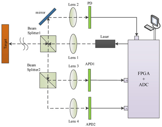
Figure 1.
The schematic diagram of pulsed LiDAR system based on differential method based on linear fitting (DMLF).
A short pulse is transmitted through the collimating lens 1, and then the pulse is divided into two beams by beam splitter1 (BS1). One beam is focused by a convergent lens 2 and is detected directly by a photodetector (PD), which generates the start signal and sets it as the start time (tt) of TOF. The other beam is used to illuminate the target. The light reflected from the object surface is divided into two parts by beam splitter2 (BS2), which are received by two APDs through a convergent lens, respectively. The two electrical signals of Prd1 and Prd2, generated by APD1 and APD2, are sent to a subtracter. We will obtain the differential pulse signal Prd1-Prd2 after the subtraction operation, and send it to the analog-to-digital converter (ADC). There is a PGZCPs between the differential pulse signal and zero axial, so we define the PGZCPs as the stop timing moment (tr) of TOF. According to the theory of TOF, the calculation formula of range is given by
where c is the velocity of light.
2.2. Model of Transmitted Pulse and Echo Pulse in LiDAR
In this section, we will describe the LiDAR pulse model during transmitted and echo process. As is known, if the trailer of a short pulse can be ignored and its normalized time-domain envelope is approximately Gaussian-shaped, it is written as
where , td is the fixed delay of transmitted pulse and is the pulse width.
During the operation of pulsed LiDAR, the echo signal reflected from target surface will be disturbed by a lot of interference, such as atmospheric attenuation, optical transmission attenuation, and target reflectivity et al. Hence, the echo pulse model can be described as [3]
where Et is the transmitted energy of LIDAR. is the two-way atmospheric transmission loss. is the transmission efficiency of the optics. AR is the receiver area of the detector. is the target’s reflectivity. is the local incidence angle. R is the distance between the target and Lthe iDAR transmitted system. Nn is random noise, which includes background noise, speckle noise, and thermal noise.
In order to calculate easily during the processing of echo signal, we use SNR to replace the , and other difficult-to-measure parameters in Equation (3). The SNR is the ratio between the mean peak power received on the detector and the root mean square (RMS) of the photo-electronic chain without signal. TNR refers to the detection threshold value to the RMS of noise ratio, written as [22]
where is the maximum detection distance, is the matched bandwidth of receiver, and is the false alarm rate within a single pulse, which determines the detecting threshold value of the effective signal VT.
We have normalized the peak value to 1 in the emission pulse model, so the noise power spectrum density of the LiDAR system becomes , where the RMS of noise amplitude is , the return pulse power spectrum density is . Therefore, the simpler echo pulse model can be expressed as
where the R refers to the distance of return signal and is for the attenuated factor.
2.3. Analysis of the Differential-Optical-Path Approach
In terms of stop-time moment, the traditional method of echo pulse can be described as Equation (5), which only uses an APD to receive the scattered light signal from the target and calculate the PPs of the echo pulse waveform. However, this method easily suffers from interference by noise and is only suitable for steep peak form.
Unlike the traditional method, the DMLF is to add a beam splitter between the convergent lens 3 and beam splitter1, where d presents the axial shift in the APD2, which is determined by the pulse width and [20]. The second APD receives the light signal derived from beam splitter2. The stop-time moment is obtained by calculating the differential of two APD signals and the differential echo pulse model can be denoted in the form of
According to Equation (6), when the , we can obtain Formula (7)
where is the zero-crossing timing moment. Due to the determined position of APD1, the axial shift d and transmitted pulse delay td are constant. Therefore, Equation (7) demonstrates that the differential method can obtain the stop-time moment, similar to the traditional method, which also proves the feasibility of the DMLF.
From the above analysis, the stop-time moment is successfully changed from PPs to PGZCPs of DMLF. Obviously, the change rates of amplitude per unit moment at the PGZCPs are higher than those at the PPs of the traditional method. Therefore, our proposed method has a higher sensitivity and more accurate timing moment.
Using Equations (6) and (7), . Let , which is a function with the variable of d. This means that the sensitivity of PGZCPs in DMLF is related to the axial shift d. Therefore, we can obtain the optimal d corresponding to the maximum sensitivity by , yielding . In order to quantitatively analyze the above theory, we carried out simulations for different axial shift d, which is shown in Figure 2a. It can be seen that as the d increases, the slope of the differential signal near PGZCPs has a tendency to increase initially and then decrease. The largest slope at , which is the optimal axial shift.
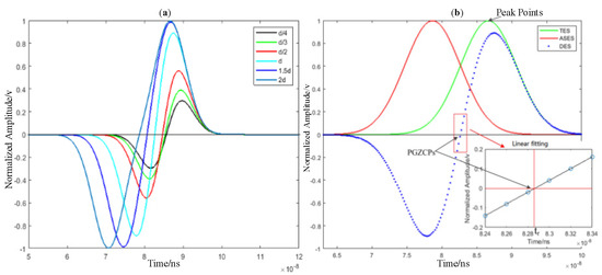
Figure 2.
(a) Differential echo pulse curves for different axial shift; (b) The traditional peak method and DMLF. TES, ASES, and DES means traditional echo signal, axial shift echo signal, and differential echo signal, respectively.
2.4. Analysis of the Linear Fitting Near PGZCPs
Through the above analysis, we already know the feasibility of the differential method and the optimal axial displacement d corresponding to the maximum sensitivity of the differential echo curve. Next, we select seven points near the PGZCPs in the differential echo signal curve to fit a line, according to the slope value k of the linear-fitting curve to verify the optimal axial shift d. The simulation results are described as Table 1. when , which also verifies the correctness of Figure 2a.

Table 1.
The slopes of linear fitting curve at different axial shift.
After period research, we find that, sometimes, the zero-crossing point maybe not exactly zero, but instead is a very small value. Therefore, in order to confirm the zero-crossing position exactly, we take the intersection of the fitting curve of the points near PGZCPs and the zero axes as the true zero point, which is the stop-time moment of TOF.
Figure 2b is shown the traditional peak method, and the DMLF echo signal curves at , tr is the stop-time moment that we expect.
2.5. DMLF Algorithm Flow Chart
Through analysis of Section 2.3 and Section 2.4, we have known that the DMLF algorithm can effectively improve the accuracy of the pulse-ranging LiDAR. In order to obtain a clearer understanding of the DMLF algorithm, we will introduce the specific process of the algorithm below. Figure 3 shows the main steps of the DMLF algorithm, which are summarized as follows.
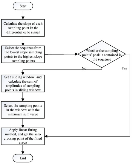
Figure 3.
Flow chart for DMLF algorithm.
First: Select the sampling points. The slope of each sampling point in the differential echo signal is measured, and the sequence of sampling points between the sampling point with the lowest slope and the sampling point with the highest slope is selected.
Second: Determine the condition of the selected sampling points. If the peak of the sampling points is included in the sequence selected in the first stage, go to the fourth stage. If not, please go to the third stage.
Third: Reselect the sampling point. Within the entire sampling points, move a time window, with the width of the time interval between the lowest-slope sampling points and the highest-slope sampling points. Select the sampling points sequence with the largest sum in the window, and then return to the fourth stage.
Fourth: Apply the linear fitting method. Finally, the stop timing moment of the echo pulse is designated as the zero-crossing point of the fitted curve.
Linear fitting is the core content of DMLF algorithm, which is related to the accuracy of pulse ranging. Therefore, the specific steps of linear fitting in this article are as follows.
Step 1: Find the sampling points sequence from the lowest-slope sampling points to the highest slope sampling points, which contain the peak.
Step 2: Search the sampling point in the sequence of sampling points whose amplitude is closest to zero.
Step 3: Seven points near the zero-sampling point are selected and a linear curve is fitted.
Step 4: It is assumed that the waveform of selected sampling points can be expressed by the following equation
The sum of the distances between the fitting datapoints and the sampled datapoints can be expressed as
where yi is the amplitude of the sampling points; a and b are the parameters of the fitting curve; xi is the time of the sampling points.
Step 5: Take the derivative of Equation (9), and we will obtain the expression for a and b as follows
where X and Y represent the mean value of xi and yi. Substituting the sampling points data into Equation (10), a and b can be obtained; thus, we will obtain the fitting curve.
Step 6: The stop-time moment is set as the time value when the fitting curve amplitude is zero
3. Results
3.1. Simulation Set Up
Based on the above theory and system flow chart, the simulation models have been set up to verify the progressiveness and accuracy of DMLF. The parameters of pulse ranging LiDAR system and target are set as the following: Et = 4.8 uJ; ; ; beam diameter is 3.0 mm; laser repetition frequency is 200 kHZ; angle of divergence is 0.51 mrad; transmitting and receiving system optical aperture are 32 and 50 mm; APD photosensitive surface size is 3.0 mm; ADC sampling rate, bandwidth and sampling digit are 5 GSa/s, 1 GHz, and 14 bit, respectively; target reflectivity ; optimal axial shift d = 1.2 m.
The waveform of the transmitted pulse and echo pulse of LiDAR system after filtering are shown in Figure 4a. Obviously, the peak point’s area of echo signal is disturbed by noise, which makes it difficult to extract useful moment information through the peak position. Therefore, the applicability of the peak method is limited.
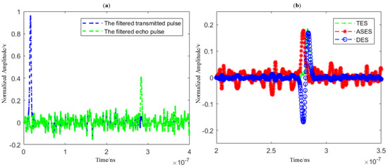
Figure 4.
(a) The filtered transmitted pulse and echo pulse in LiDAR system; (b) Simulation results of echo pulse profile.
In this situation, the differential method based on linear fitting is used, and the simulation results are shown in Figure 4b. We use the differential method to change PPs into PGZCPs, and then calculate the true stop-time moment by the linear fitting curve of points near PGZCPs.
The reflectivity of different objects varies greatly. Asphalt and cement objects have a low reflectivity approximately 0.2, and the automobile surface metal plate has a higher reflectivity, about 0.75. Therefore, in order to verify the high efficiency of the DMLF algorithm in this paper, we applied it to different reflectivity conditions for simulation, and the simulation results are shown in the Appendix A.
Considering the effect of noise, we carry out simulation experiments 1000 times with an SNR of 5–15 dB, and range from 30 to 50 m, respectively. The noise added in the simulation is Gaussian white noise with the same mean value. The performance of the peak method and the proposed DMLF will be further compared and analyzed below.
3.2. Error Analysis
We performed 1000 simulation experiments on the peak method and the proposed DMLF with 1 dB and 1 m steps, respectively. The difference between the measured value and the true value is called error; we analyzed the Root Mean Square Error (RMSE) and Relative Error (RE) in the experimental results, which is shown in Figure 5 and Figure 6.
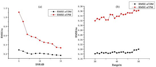
Figure 5.
(a) The RMSE of DMLF with the change in SNR. (b) The RMSE of tradition PM with the change in Range. DM means the proposed DMLF, and PM means peak method.
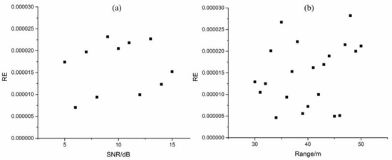
Figure 6.
(a) RE of DMLF in different SNR. (b) RE of DMLF in different Ranges.
Obviously, in Figure 5a, the proposed DMLF has a higher timing accuracy than the traditional method, no matter which levels of SNR are used, and with the increase in SNR, the RMSE of peak method and DMLF are decreased. When the SNR = 15 dB, the traditional peak method has an RMSE of about 0.3318 ns, while it is about 0.1661 ns for proposed DMLF, which means that the error could be reduced by about 50% if we use the latter one. When the SNR changes from 5 to 7 dB, the RMSE of the traditional method decreases sharply, almost from 1.1113 ns to 0.6264 ns, which shows that the effect of this method is very unsatisfactory in the case of a low SNR level. This sharp change in error in the traditional method is due to the peak area of the echo signal becoming severely damaged under the condition of low SNR, and the sensitivity of the peak point’s area is too low. On the contrary, our method is still lower than 0.3 ns. In Figure 5b, the proposed DMLF also shows good timing accuracy, and the fluctuation with distance is also smaller than in the traditional method. When the distance is 50 m, the traditional peak method has an RMSE of about 0.3625 ns, while, it is about 0.1999 ns for the proposed DMLF. This sufficiently proves that our proposed method is more robust to noise and has better timing accuracy.
We also analyzed the RE of the proposed DMLF at different SNR and ranges. As shown in Figure 6, it can be seen that, under the experimental conditions, the RE can be maintained from 4 to 29 ppm. Considering other environmental or negligible errors, the RE of DMLF can be less than 30 ppm.
4. Conclusions
In this paper, a novel pulsed-laser ranging system of the differential methods based on linear fitting is proposed, and a mathematical model is established and verified. Compared with the traditional peak method with a single APD receiver, DMLF obtains the echo signal through two APD receivers and acquires the differential signal through a subtracter. Therefore, the PPs are changed to PGZCPs. Simulation experiments show that PGZCPs has higher sensitivity. We can also obtain the highest sensitivity when the axial shift . According to the above simulation and analysis, the proposed DMLF could improve the timing accuracy of laser ranging. Additionally, there are some obvious advantages to our approach:
- (1)
- It can handle phenomena such as low SNR and high noise power, and has strong anti-interference ability and robustness;
- (2)
- Compared with the traditional peak method, the DMLF proposed in this paper can reduce the timing error and decrease the RMSE by almost 50%;
- (3)
- Using the differential method with optimal axial shift d, the sensitivity and ranging accuracy of the pulse ranging LiDAR are significantly improved, and the RE of ranging can be less than 30 ppm.
Therefore, based on the above summary, our proposed method has a few advantages in improving the accuracy of the laser pulse-ranging system.
In this paper, our works aim to establish a mathematical model of the proposed method and perform a simulation to verify the feasibility, and experimental verification will be carried out in our future works.
Author Contributions
Conceptualization: D.G.; data curation: D.G., B.Q.; formal analysis: D.G., B.Q.; funding acquisition: C.W.; investigation: D.G.; methodology: D.G. and B.Q.; resources: C.W.; software: D.G.; supervision: C.W.; validation: D.G. and B.Q.; visualization: D.G.; writing—original draft: D.G. writing—review and editing: D.G. and B.Q. All authors have read and agreed to the published version of the manuscript.
Funding
This research was funded by the Shenzhen Fundamental Research Program (Grant No.JCYJ2020109150808037); the National Key Scientific Instrument and Equipment Development Projects of China (Grant No.62027823); the National Natural Science Foundation of China (Grant No.61775048).
Institutional Review Board Statement
Not applicable.
Informed Consent Statement
Not applicable.
Data Availability Statement
Not applicable.
Conflicts of Interest
The authors declare no conflict of interest.
Appendix A
In order to verify the robustness of the DMLF algorithm in this paper, we have simulated the pulse waveforms under different target reflectivity, and the results are shown as follows.
In Figure A1, the reflectivity from the first row to the fourth row are 0.2, 0.4, 0.6, and 0.8, respectively. The first column is the transmitted and echo pulses after filtering under different reflectivity conditions, and the second column is the comparison between the traditional peak method and DMLF.
It can be seen from the figure that the target’s echo pulse amplitude is positively correlated with the surface reflectivity, and in any case, the DMLF algorithm performs well, which further proves the efficiency and robustness of the algorithm.

Figure A1.
Simulation under different reflectivity conditions. (a,c,e,g) is the transmitted and echo pulses after filtering under the reflectivity of 0.2, 0.4, 0.6 and 0.8; (b,d,f,h) is the comparison between the traditional peak method and DMLF under the reflectivity of 0.2, 0.4, 06, and 0.8.
References
- Xu, F.; Wang, Y.; Yang, X.; Zhang, B.; Li, F. Correction of linear-array lidar intensity data using an optimal beam shaping approach. Opt. Lasers Eng. 2016, 83, 90–98. [Google Scholar] [CrossRef]
- McManamon, P.F. Errata: Review of ladar: A historic, yet emerging, sensor technology with rich phenomenology. Opt. Eng. 2012, 51, 060901. [Google Scholar] [CrossRef]
- Richmond, R.D.; Cain, S.C. Direct-Detection LADAR Systems; SPIE: Bellingham, WA, USA, 2010. [Google Scholar]
- Ma, X.; Wang, C.; Han, G.; Ma, Y.; Li, S.; Gong, W.; Chen, J. Regional Atmospheric Aerosol Pollution Detection Based on LIDAR Remote Sensing. Remote Sens. 2019, 11, 2339. [Google Scholar] [CrossRef]
- Xing, Y.; Huang, J.; Gruen, A.; Qin, L. Assessing the Performance of ICESat-2/ATLAS Multi-Channel Photon Data for Estimating Ground Topography in Forested Terrain. Remote Sens. 2020, 12, 2084. [Google Scholar] [CrossRef]
- Royo, S.; Ballesta-Garcia, M. An overview of lidar imaging systems for autonomous vehicles. Appl. Sci. 2019, 9, 4093. [Google Scholar] [CrossRef]
- Pimentel, J.; Bastiaan, J. Characterizing the safety of self-driving vehicles: A fault containment protocol for functionality involving vehicle detection. In Proceedings of the 20th IEEE International Conference on Vehicular Electronics and Safety (ICVES), Conference Proceedings, Madrid, Spain, 12–14 September 2018; pp. 12–14. [Google Scholar]
- Yan, Z.; Duckett, T.; Bellotto, N. Online learning for 3D LiDAR-based human detection: Experimental analysis of point cloud clustering and classification methods. Auton. Robot. 2020, 44, 147–164. [Google Scholar] [CrossRef]
- Pan, Z.; Glennie, C.; Hartzell, P.; Fernandez-Diaz, J.C.; Legleiter, C.; Overstreet, B. Performance assessment of high resolution airborne full waveform LiDAR for shallow river bathymetry. Remote Sens. 2015, 7, 5133–5159. [Google Scholar] [CrossRef]
- Xia, W.; Han, S.; Cao, J.; Yu, H. Target recognition of log-polar ladar range images using moment invariants. Opt. Lasers Eng. 2017, 88, 301–312. [Google Scholar] [CrossRef]
- Suchocki, C.; Damięcka-Suchocka, M.; Katzer, J.; Janicka, J.; Rapiński, J.; Stałowska, P. Remote Detection of Moisture and Bio-Deterioration of Building Walls by Time-Of-Flight and Phase-Shift Terrestrial Laser Scanners. Remote Sens. 2020, 12, 1708. [Google Scholar] [CrossRef]
- Xu, L.; Zhang, Y.; Zhang, Y.; Wu, L.; Yang, C.; Yang, X.; Zhang, Z.; Zhao, Y. Signal restoration method for restraining the range walk error of Geiger-mode avalanche photodiode LIDAR in acquiring a merged three dimensional image. Appl. Opt. 2017, 56, 3059–3063. [Google Scholar] [CrossRef] [PubMed]
- Whyte, R.; Streeter, L.; Cree, M.J. Application of LIDAR techniques to time-of-flight range imaging. Appl. Opt. 2015, 54, 9654–9664. [Google Scholar] [CrossRef] [PubMed]
- Hintikka, M.; Hallman, L.; Kostamovaara, J. Comparison of the leading-edge timing walk in pulsed TOF laser range finding with avalanche bipolar junction transistor (BJT) and metal-oxide-semiconductor (MOS) switch based laser diode drivers. Rev. Sci. Instrum. 2017, 88, 123109. [Google Scholar] [CrossRef] [PubMed]
- Kurtti, S.; Kostamovaara, J. An integrated receiver channel for a laser scanner. In Proceedings of the IEEE International Instrumentation and Measurement Technology Conference (I2MTC), Graz, Austria, 13–16 May 2012; pp. 1358–1361. [Google Scholar]
- Li, X.; Wang, H.; Yang, B.; Huyan, J.; Xu, L. Influence of time-pickoff circuit parameters on LiDAR range precision. Sensors 2017, 17, 2369. [Google Scholar] [CrossRef] [PubMed]
- Chevalier, T.R.; Steinvall, O.K. Laser radar modeling for simulation and performance evaluation. In Proceedings Electro-Optical Remote Sensing, Photonic Technologies, and Applications III; International Society for Optics and Photonics: Berlin, Germany, 2009; Volume 7482, p. 748206. [Google Scholar]
- Zhang, Z.; Zhao, Y.; Zhang, Y.; Wu, L.; Su, J. A real-time noise filtering strategy for photon counting 3D imaging LIDAR. Opt. Express 2013, 21, 9247–9254. [Google Scholar] [CrossRef] [PubMed]
- Qin, Y.C.; Vu, T.T.; Ban, Y.; Niu, Z. Range determination for generating point clouds from airborne small footprint LiDAR waveforms. Opt. Express 2012, 20, 25935–25947. [Google Scholar] [CrossRef] [PubMed]
- Yang, J.; Qiu, L.; Zhao, W.; Wu, H. Laser differential reflection-confocal focal-length measurement. Opt Express 2012, 20, 26027–26036. [Google Scholar] [CrossRef] [PubMed]
- Zhao, W.; Sun, R.; Qiu, L. Laser differential confocal ultra-long focal length measurement. Opt Express 2009, 17, 20051–20062. [Google Scholar] [CrossRef] [PubMed]
- Li, Y.X.; Cui, T.X.; Li, Q.Y.; Zhang, B.; Bai, Y.R.; Wang, C.H. Waveform centroid discrimination of return pulse weighting method in LIDAR system. Optik 2019, 180, 840–846. [Google Scholar] [CrossRef]
Publisher’s Note: MDPI stays neutral with regard to jurisdictional claims in published maps and institutional affiliations. |
© 2021 by the authors. Licensee MDPI, Basel, Switzerland. This article is an open access article distributed under the terms and conditions of the Creative Commons Attribution (CC BY) license (http://creativecommons.org/licenses/by/4.0/).