Automated Accuracy Assessment of a Mobile Mapping System with Lightweight Laser Scanning and MEMS Sensors

Abstract

The accuracy assessment of mobile mapping system (MMS) outputs is usually reliant on manual labor to inspect the quality of a vast amount of collected geospatial data. This paper presents an automated framework for the accuracy assessment and quality inspection of point cloud data collected by MMSs operating with lightweight laser scanners and consumer-grade microelectromechanical systems (MEMS) sensors. A new, large-scale test facility has been established in a challenging navigation environment (downtown area) to support the analyses conducted in this research work. MMS point cloud data are divided into short time slices for comparison with the higher-accuracy, terrestrial laser scanner (TLS) point cloud of the test facility. MMS data quality is quantified by the results of registering the point cloud of each slice with the TLS datasets. Experiments on multiple land vehicle MMS point cloud datasets using a lightweight laser scanner and three different MEMS devices are presented to demonstrate the effectiveness of the proposed method. The mean accuracy of a consumer grade MEMS (<$100) was found to be 1.13 ± 0.47 m. The mean accuracy of two commercial MEMS (>$100) was in the range of 0.48 ± 0.23 m to 0.85 ± 0.52 m. The method presented here in can be straightforwardly implemented and adopted for the accuracy assessment of other MMSs types such as unmanned aerial vehicles (UAV)s.

1. Introduction

A mobile mapping system (MMS) can be defined as an integrated sensing system for the collection of geospatial data from a moving platform. At its core, an MMS comprises an integrated GNSS/IMU system for determination of the platform state and one or more imaging sensors. It may include additional navigation sensors such as a wheel revolution counter. The trajectory estimates from the navigation system allow direct georeferencing of acquired image data. The two main types of imaging sensors found on board MMSs are passive cameras and laser scanners. Since the focus of this work is the latter, an MMS is henceforth understood to mean a laser scanning based system. Early MMSs were developed for land-vehicle platforms but have since evolved into backpack, hand cart, water vehicle and unmanned aerial vehicle (UAV) embodiments in support of a vast range of applications. The work described herein focuses on a land-vehicle MMS accuracy testing, though the methods are expected to be broadly applicable to other platforms such as UAVs with suitable adaptation.

According to [1], MMSs may be classified according to the accuracy they can achieve, either mapping or survey grade. Achieving the higher, survey-grade accuracy relies on accurate trajectory determination, which is particularly challenging in GNSS-denied and multipath environments such as urban canyons. Kersting and Friess [1] report a post-mission quality assurance procedure for survey-grade MMSs. They perform a fully automated self-calibration to estimate corrections to system parameters (boresight and lever arm) and corrections to the trajectory. Planar features are used for the self-calibration. The plane-based system calibration method has been used for airborne [2], UAV [3] and mobile [4,5] laser scanner systems and the modelling has been extended to include catenary curves [6] and poles [7]. The trajectory model reported by [1] includes a second-order corrections as a function of time. The trajectory is segmented according to position accuracy to allow piecewise modelling with continuity and smoothness constraints.

Methods to assess and improve the accuracy of MMSs have been investigated by many authors. Signalized control points [8] and signalized tie points [9] observed in multiple MMS passes have been reported to correct navigation system errors while check points [10] can be employed to independently quantify the errors. The use of total stations and GNSS equipment results in accurately determined point coordinates [11]. However, point-based assessment suffers from the great disparity in data density between the MMS and the independently surveyed points.

In recognition of this shortcoming, a number of researchers have developed outdoor test fields for MMS accuracy assessment. Generally speaking, they comprise a dense reference point cloud of a large urban area through which the MMS can be driven. The reference point cloud is collected by static terrestrial laser scanning (TLS) that is georeferenced with static or RTK GNSS methods. The accuracy assessment of MMS data can be performed by comparing the two point clouds, though the features and methods used for comparison vary.

Kaartinen et al. [12] detail the testing of several MMSs over a 1.7 km loop. They quantify system accuracy by comparing the coordinates of independently surveyed point features. The reference targets are poles, building corners and curb corners extracted from the point cloud. Xu et al. [13] report a mobile laser scanner test field of similar size (1000 m × 550 m area). Their assessment is conducted with 45 control points. Fryskowska and Wróblewski [14] also use TLS data as a reference to assess the accuracy of an MMS. Their assessment is performed using a large number of check points and the lengths of building features. In their manual for laser-based mobile mapping, Johnson et al. [15] report two test sites (urban and rural) established with control points for performance testing of MMSs. Both sites are about 3 km long. Accuracy is assessed with signalized control points and TLS reference data. The latter source is used at a specific site to estimate bridge clearance. Toschi et al. [16] use TLS reference data collected of two buildings in a city center to evaluate MMS accuracy. Iterative closest point (ICP) method registration [17] is performed on segmented building data and various statistical measures, including higher-order moments, are computed for the assessment. Rodríguez-Gonzálvez et al. [18] constructed a 2.5 km long TLS point cloud of a medieval wall for the accuracy assessment of their MMS. However, the assessment was performed over a small section of the wall.

The accuracy assessment of indoor MMSs (IMMS) is described by [19]. Three IMMSs were tested using a pre-surveyed cultural heritage site as a reference test field. TLS data of the test field serves as ground truth. IMMS data were collected on two pre-defined paths: one closed and one open. Subsets of the data were registered to reference data by the ICP method. A number of different data comparisons are reported to quantify the accuracy of each system.

The assessment of MMS accuracy is not, however, confined to the built environment. Rönnholm et al. [20] evaluate the quality of backpack laser MMS in a forest relative to reference data collected with UAV and TLS. The evaluation is performed by comparing data patches comprising 10 s of data with ICP. The time series duration is a tradeoff between enough topographic variation in the data and changes in system orientation. Performing independent ICPs creates discontinuities between patches, so the parameters of adjacent patches are (linearly) time dependent.

The past decade has seen tremendous growth in the utilization of unmanned aerial vehicles for airborne mapping. Though cameras are ubiquitous sensors found onboard mapping UAVs, the deployment of light-weight laser scanner systems is becoming more commonplace. Accordingly, the assessment of the accuracy of point clouds derived from such systems is of great importance. Perhaps not surprisingly, the use of an independently observed reference point cloud has been employed by a number of researchers. Several different laser scanner systems appear in the literature including the ibeo LUX LiDAR sensor [21], the SICK LMS511 PRO [22], the RIEGL miniVUX lidar [23] as well as the HDL-32E [24], the VLP-16 Puck HI-RES [3] and the VLP-16 [25] models from Velodyne.

Bakuła et al. [21] report on the assessment of UAV point cloud accuracy in support of levee monitoring using signalized points and cross sections. This group utilizes airborne laser scanner and ground survey data for a later assessment [25]. A multi-faceted assessment of UAV laser scanner data quality over a landslide area is described by [23]. Assessments of strip adjustment quality, overall digital elevation model accuracy, point density and change detection were conducted by comparing the UAV data with TLS, total station and GNSS data. The use of TLS point clouds of single buildings and their surroundings as the reference data are reported by [22,24].

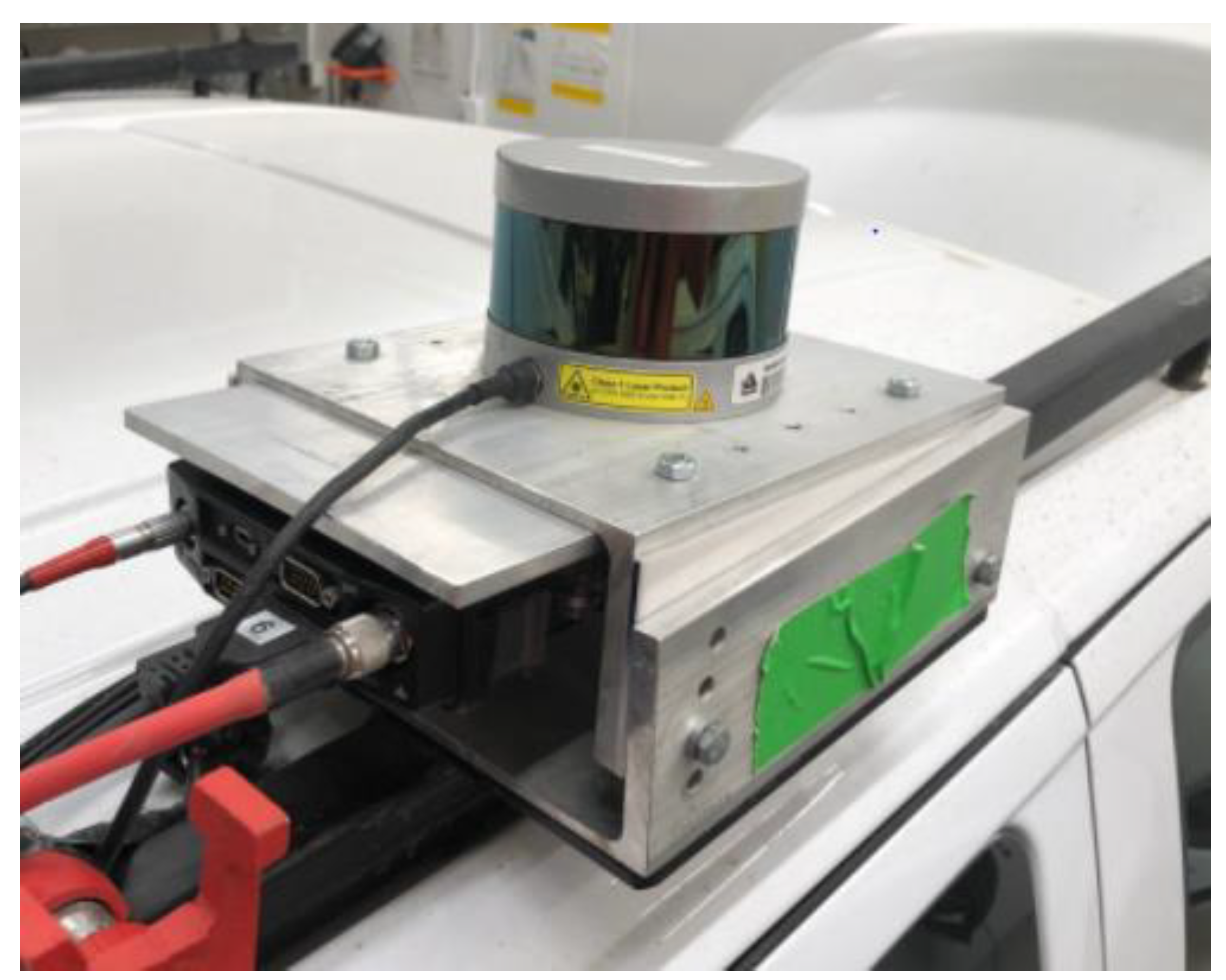
Clearly, recent activities found in the literature indicate the importance of evaluating the metric performance of lightweight laser scanning systems utilized in MMSs regardless of whether they are deployed on a land vehicle or a UAV platform. This need is further emphasized with the increased use of low-cost microelectromechanical systems (MEMS) sensors in the navigation system. This work presents the design of a completely automated framework for land-vehicle MMS accuracy assessment by comparing a mobile laser scanner point cloud with a reference point cloud of a dedicated testing facility. The establishment of the testing facility comprising several downtown city blocks—a challenging GNSS environment—is also detailed. Multiple datasets with an MMS fitted with a Velodyne VLP-16 and three different MEMS sensors were captured to demonstrate the effectiveness of the proposed method. Detailed evaluation of these sensors is presented following the experiment description.

2. Methodology

Before describing the proposed methodology for lightweight laser scanner performance assessment, it is important to review the kinematic MMS positioning equation. The mapping frame coordinates (m) of a point p, $r_p^m\left(t\right)$, observed by an MMS, can be expressed as follows:

$$r_p^m\left(t\right)=r_b^m\left(t\right)+R_b^m\left(t\right)\left\{a_{IMU/s}^b+R_s^b{r}_p^s\left(t\right)\right\}$$

(1)

where $r_b^m\left(t\right)$ is the position of the body frame (b) origin; $R_b^m\left(t\right)$ is the body frame attitude matrix, which is parameterized in terms of the time-varying roll, pitch and yaw angles, and represents the rotational transformation from the body frame to the mapping frame; $a_{IMU/s}^b$ is the lever arm offset vector between the sensor (laser scanner) frame (s) and the body frame (the IMU axes); $R_s^b$ is the boresight matrix, parameterized in terms of three Cardan angles, which represents the rotation from the sensor frame to the body frame; and $r_p^s\left(t\right)$ is the position vector of point p in the sensor frame. For a Velodyne laser scanner, the vector $r_p^s\left(t\right)$ is a function of the observed range, rotation angle and the vertical angle of each of its 16 lasers as well the scanner’s interior calibration parameters. Additional details about the laser scanner are given later.

All quantities are considered to time-varying except for the elements of the boresight matrix and the lever arm vector, which are pre-calibrated and treated as constants. The mapping frame in this project was the 3TM projection with central meridian 114° west. The point coordinates given by Equation (1) are prone to many error sources. If the mounting parameters (boresight and lever arm) have been accurately calibrated, then the errors can be attributed to the navigation and laser scanner systems. MMS position and orientation can be severely biased in GNSS-denied and high-multipath environments like urban canyons. They can rapidly vary with time if a low-cost IMU is used.

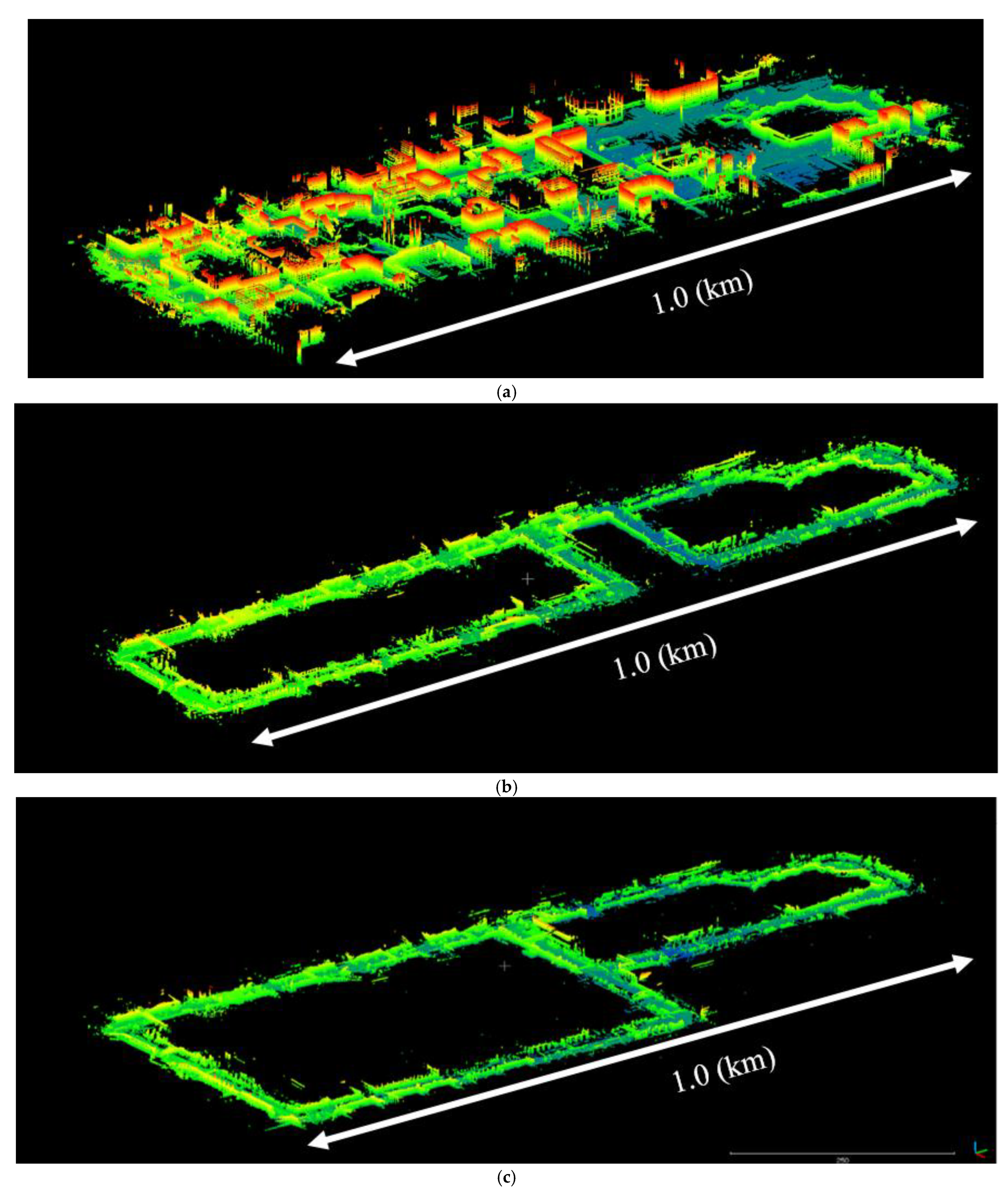
The accuracy assessment methodology is based on spatial comparison of an MMS (kinematic) point cloud and a GNSS/IMU-independent (static) point cloud. The kinematic point cloud possesses variable spatial accuracy at different temporal points due to the nature of the MMS data collection. For instance, areas with sufficient GNSS coverage feature high spatial quality, while areas with a lack of GNSS coverage may feature lower spatial quality, depending on the aiding provided by the IMU for the navigation solution. On the other hand, the static point cloud possesses almost constant accuracy since it is based on a precise multi-station terrestrial laser scanning survey that does not rely on kinematic GNSS/IMU position and orientation estimates. A spatial comparison between the kinematic point cloud and the static one will indicate any discrepancies between the two datasets.

One famous way to derive spatial discrepancies between point clouds is by conducting 3D registration [26]. The well-known iterative closest point method [17] can handle registration between point clouds from different sources and with variable point density. The application of the ICP-registration results in six Helmert transformation parameters (i.e., three translations and three rotation angles), which are used as the accuracy measure for the spatial quality of the kinematic point cloud. The scale parameter is not solved for using the ICP since the laser scanners preserve unit scale factor. If the kinematic point cloud has a high spatial quality, it will match the static point cloud and the values of the six transformation parameters will be close to zeroes following the ICP registration. Any differences between the two point-clouds will be indicated by large, non-zero values for the transformation parameters.

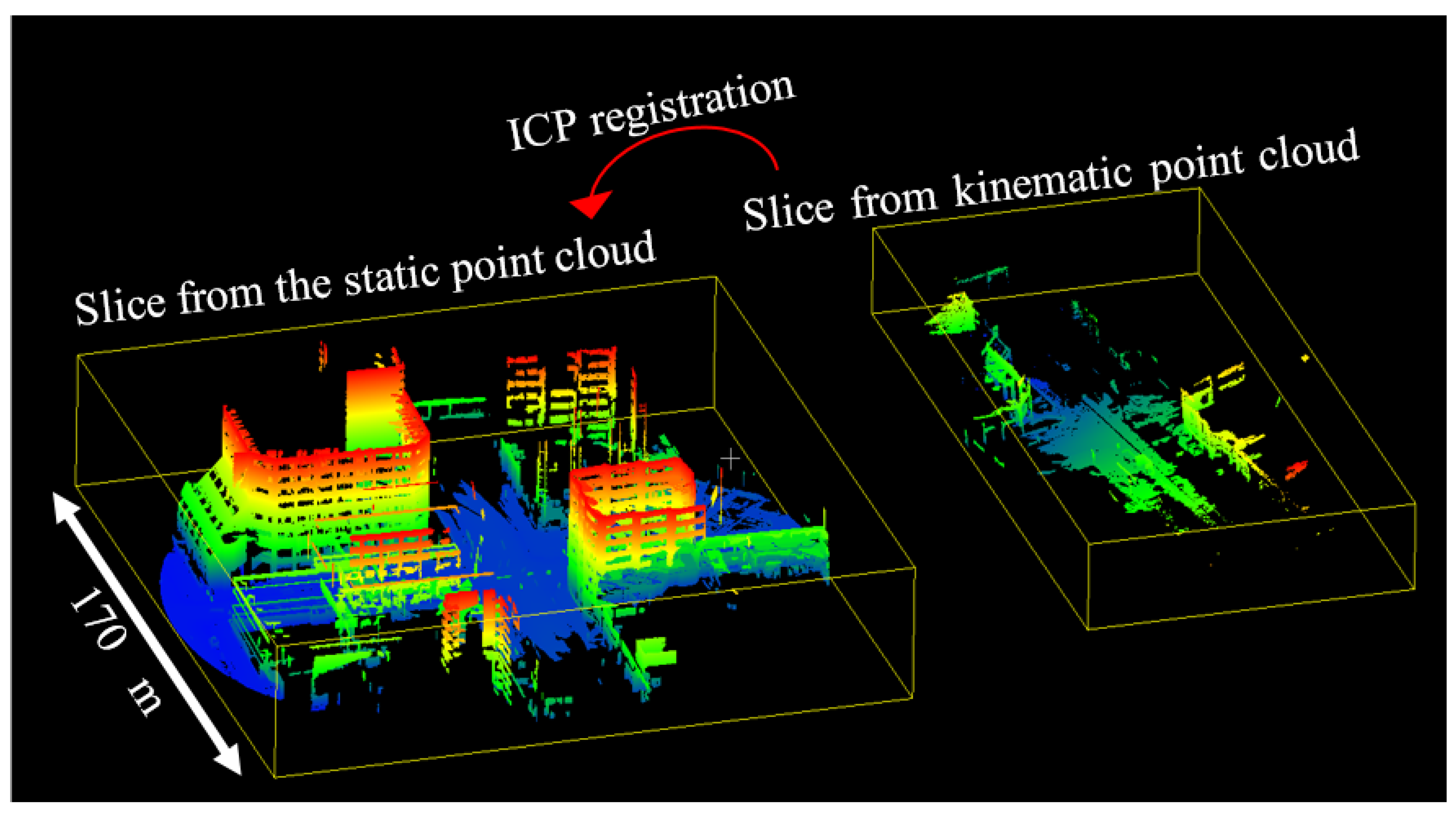
For a rigorous accuracy assessment, the kinematic point cloud is divided into temporal slices prior to the registration. Each temporal slice contains points from a short time interval of data collection. The individual slices are sequentially registered to the static point cloud using the ICP (Figure 1). The functional relationship between a point in the cloud captured by the MMS in slice k, $r^{MMS}$, and the closest point in the reference TLS point cloud, $r^{TLS}$, is thus given by:

$$r^{TLS}=R_k{r}^{MMS}+t_k$$

(2)

where $t_k$ is the translation vector and $R_k$ is the rotation matrix between the two point clouds. Note that the mapping frame superscript has been omitted for clarity. The objective of the ICP is to minimize the sum of squares of differences between the two point clouds, ε², i.e.,

$${\epsilon }^2={\displaystyle \sum {\Vert R_k{r}^{MMS}+t_k-r^{TLS}\Vert }^2}$$

(3)

It is assumed that the initial position and orientation of the kinematic point cloud provided by the direct georeferencing is sufficiently accurate enough to ensure convergence of the ICP. The result of applying this procedure to all slices is a time-series of transformation parameter sets that provides an accuracy measure of the kinematic data at different temporal points and spatial locations.

Note that navigation quality changes rapidly in urban areas and, accordingly, the spatial quality of the kinematic point cloud may vary at different temporal points. Therefore, it is hypothesized that a shorter temporal slice will result in a more realistic accuracy assessment. Point cloud data collected within a short time interval from a moving mobile mapping system will have homogeneous spatial accuracy. Nevertheless, one should bear in mind that a very short time interval may not contain a sufficient number of points or enough objects/features to perform the ICP registration. On the other hand, a very long time interval will provide a large size point cloud with inhomogeneous spatial accuracy and may lead to a false accuracy assessment. Spatial errors in a few locations may not be detected through the registration of large point clouds. The errors may be distributed throughout the larger dataset and will not contribute significantly to the estimation of the transformation parameters. Since the transformation parameters are used to quantify data quality, a long time interval must be avoided. A few factors should be taken to account for determining the time interval length, for instance: (1) the mobile mapping system speed, (2) the laser scanner range, (3) the scanning frequency, (4) the quality of the GNSS/IMU system, and (5) the structure of the scanning area.

3. Experiment Description

3.1. Test Facility Establishment

Static and kinematic point cloud data captured over a newly established testing facility were used in this experiment. Pictured in Figure 2, the testing facility is located in the downtown area (central business district, CBD) of Calgary, Canada. It is comprised of two loops with a combined length of approximately 2.4 km long. Importantly, it passes through a variety of different urban environments including both open sky conditions and narrow urban canyons defined by high-rise buildings between 9 Ave SW, 2 St SW, 3 Ave SW and Barclay Parade SW.

The test facility was scanned by a professional surveying company using a RIEGL VZ400 terrestrial laser scanner (RIEGL Laser Measurement Systems GmbH, Horn, Austria). The static cloud comprised 184 scans that were registered into a common external coordinate system courtesy of a network of 38 control points surveyed by total station. The network was georeferenced by real-time kinematic GNSS observations of six of the control points located in open sky conditions. The georeferenced scanner data were validated at 173 independently determined points and cross sections in terms of the absolute value of coordinate differences, Δ. As can be seen from the statistical summary in

Table 1. Accuracy and precision analysis of the static, reference point cloud. Percentages indicate the proportion of coordinate differences lying within each indicated range.

	Δ ≤ 0.015 m	0.015 m ≤ Δ ≤ 0.025 m	Δ ≥ 0.025 m
Accuracy
Horizontal	87.50%	10.60%	1.90%
Vertical	100.00%	0.00%	0.00%
Precision
Horizontal	78.30%	17.40%	4.30%
Vertical	98.10%	1.90%	0.00%

, the point cloud quality is very high and more than sufficient for the assessment of MEMS-based, lightweight laser scanner MMS accuracy.

3.2. Experiment Details

The goal of this experiment was to evaluate the accuracy of the kinematic point-cloud collected from different sensors using the proposed ICP-based accuracy assessment method. Six kinematic point cloud datasets of the test facility acquired with different navigation sensors were evaluated against the static point cloud. The full area static and kinematic point clouds are shown in Figure 3.

The MMS comprises a Velodyne VLP-16 (Velodyne Lidar, San Jose, CA, USA) deployed in tandem with a NovAtel SPAN system (Novatel Inc., Calgary, AB, Canada), a tightly coupled GNSS/IMU system that includes a multi-frequency, multi-constellation receiver and an IMU. The Velodyne VLP-16 sensor comprises a vertical array of 16 lasers with an angular spacing such that the field-of-view is approximately 30°. Continuous rotation of the laser array about the sensor’s vertical axis allows collection of a panoramic point cloud. The system was fitted with three different IMUs for testing: an InvenSense IAM20680 (InvenSense Inc., City San Jose, CA, USA); an Epson G320N (Seiko Epson Corporation, Nagano, Japan); and a Honeywell HG4930 AN01 (SPAN-CPT7; Honeywell International Inc., Charlotte, NC, USA). The InvenSense falls into the consumer MEMS (<$100) category while the other IMUs are commercial MEMS (>$100).

The datasets were captured with three different test setups on 21 March, 29 October, and 31 October 2019. Figure 4 shows an example of the instrumentation setup. For the first data collection, the Invensens was mounted on the same base plate as the VLP-16 and the Epson was on a different plate but along the same beam. The second and third data collections included both the Honeywell and Epson on the same base plate as the VLP-16. The weather conditions were all similar for the three data collections, no rain or snow was present. For each dataset, a reference trajectory was determined using a Honeywell LASEREF V Micro Inertial Reference System (μIRS; Honeywell International Inc., Charlotte, NC, USA). This navigation-grade IMU provides high-accuracy trajectory data to allow quantification of MMS georeferencing accuracy independent of the Velodyne.

The proposed methodology was applied on the six kinematic data clouds one at a time. Different time intervals were tested to quantify the impact of temporal slice length on the accuracy assessment results. Each cloud was sliced based on 5 s and 10 s time interval lengths. An example of kinematic point cloud slicing with 5 s time interval is shown in Figure 5. Areas with no overlap with the static cloud have been excluded from testing. In some locations, the ICP did not converge. These slices were excluded from the analysis as they did not have strong point geometry due to excessive clutter and areas with insufficiently geometric features to allow registration of the point clouds. For this project, the registration results were inspected visually to ensure proper alignment between the kinematic and the static data. The length of the translation vector, $t_k$, that has been determined for each slice from the registration was used to create color maps at the locations of the slice center.

4. Experiment Results and Discussion

The assessment commences with analysis of the trajectory accuracy as determined with respect to the μIRS reference. Statistics of the 3D position differences for each dataset were computed over short time intervals. Typical values from each dataset are presented in

Table 2. Three-dimensional trajectory difference statistics computed in a local level frame with respect to the Honeywell LASEREF V Micro Inertial Reference System (μIRS) reference trajectory.

MEMS Sensor	# of Epochs	Mean Error (m)	Min Error (m)	Max Error (m)	Standard Deviation (m)
InvenSense	7260	2.67	0.57	5.58	1.35
Epson_1	7260	1.15	0.01	3.54	0.88
Epson_2	8250	1.09	0.00	2.86	0.77
Epson_3	7550	1.42	0.01	4.38	0.96
Honeywell_1	8250	0.39	0.00	1.22	0.31
Honeywell_2	7550	0.85	0.01	4.14	0.62

. Sub-meter accuracy (in terms of mean value) was achieved with the Honeywell IMU, while the Epson provided roughly meter-level accuracy. The mean value from the Invensens was above 2 m.

The accuracy assessment over the six kinematic point clouds resulted in a wide range of values for $t_k$ depending on the MMS’s location within the testing facility. The results are statistically summarized in

Table 3. Accuracy statistics—5 s slice length.

MEMS Sensor	Slice Count	Mean Error (m)	Min Error (m)	Max Error (m)	Standard Deviation (m)
InvenSense	93	1.13	0.08	1.89	0.47
Epson_1	108	0.83	0.17	1.80	0.37
Epson_2	107	0.85	0.05	1.84	0.52
Epson_3	109	0.75	0.09	1.70	0.45
Honeywell_1	98	0.48	0.08	1.14	0.23
Honeywell_2	106	0.85	0.07	1.78	0.42

and

Table 4. Accuracy statistics—10 s slice length.

MEMS Sensor	Slice Count	Mean Error (m)	Min Error (m)	Max Error (m)	Standard Deviation (m)
InvenSense	55	1.12	0.12	1.90	0.48
Epson_1	57	0.83	0.17	1.62	0.37
Epson_2	62	0.87	0.05	1.79	0.53
Epson_3	62	0.76	0.13	1.49	0.43
Honeywell_1	57	0.54	0.10	1.13	0.31
Honeywell_2	59	0.84	0.07	1.71	0.42

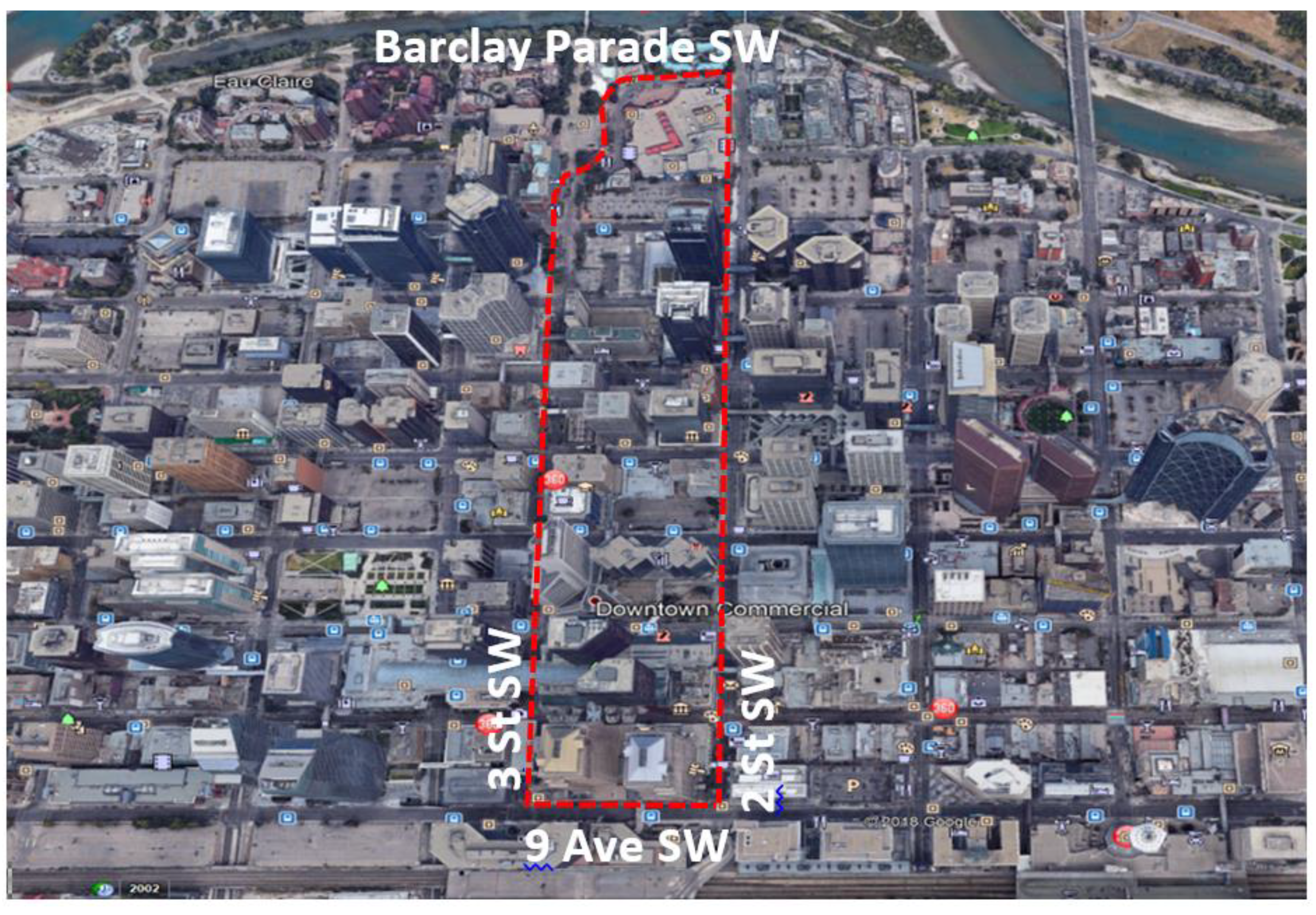
and depicted graphically in Figure 6 and Figure 7. For the six datasets, high spatial accuracy values were found in areas with good navigation conditions (open sky, no sharp turns). These outcomes were found at the northern extent of the test field in the vicinity of Barclay Parade. The land uses in this region comprise a mixture of low-rise commercial and residential buildings (two to three stories). On the contrary, but not surprisingly, lower spatial accuracy values mainly occur in the southern part of the test field where the land use is predominantly high-rise buildings that occlude the GNSS signals and degrade the navigation solution.

As can be seen in Table 3, the six point clouds provided a wide range of mean accuracy values depending mainly on the sensor type and the scanning experiment. The Epson and CPT sensors showed error magnitudes in the range of 0.48 m to 0.85 m. The InvenSense MEMS sensor produced a mean error of 1.13 m.

It is evident that the slice size did not significantly impact the accuracy assessment mean values. A comparison of the results in Table 3 and Table 4 reveals that the 5 and 10 s slice lengths provide very similar mean error values. The differences are on the order of a few centimeters, which are not significant in relation to the overall magnitude of the mean errors themselves. The differences in mean error values can be attributed to differences in the point cloud shapes for different slice sizes, which slightly impacts the quality of registration for each slice.

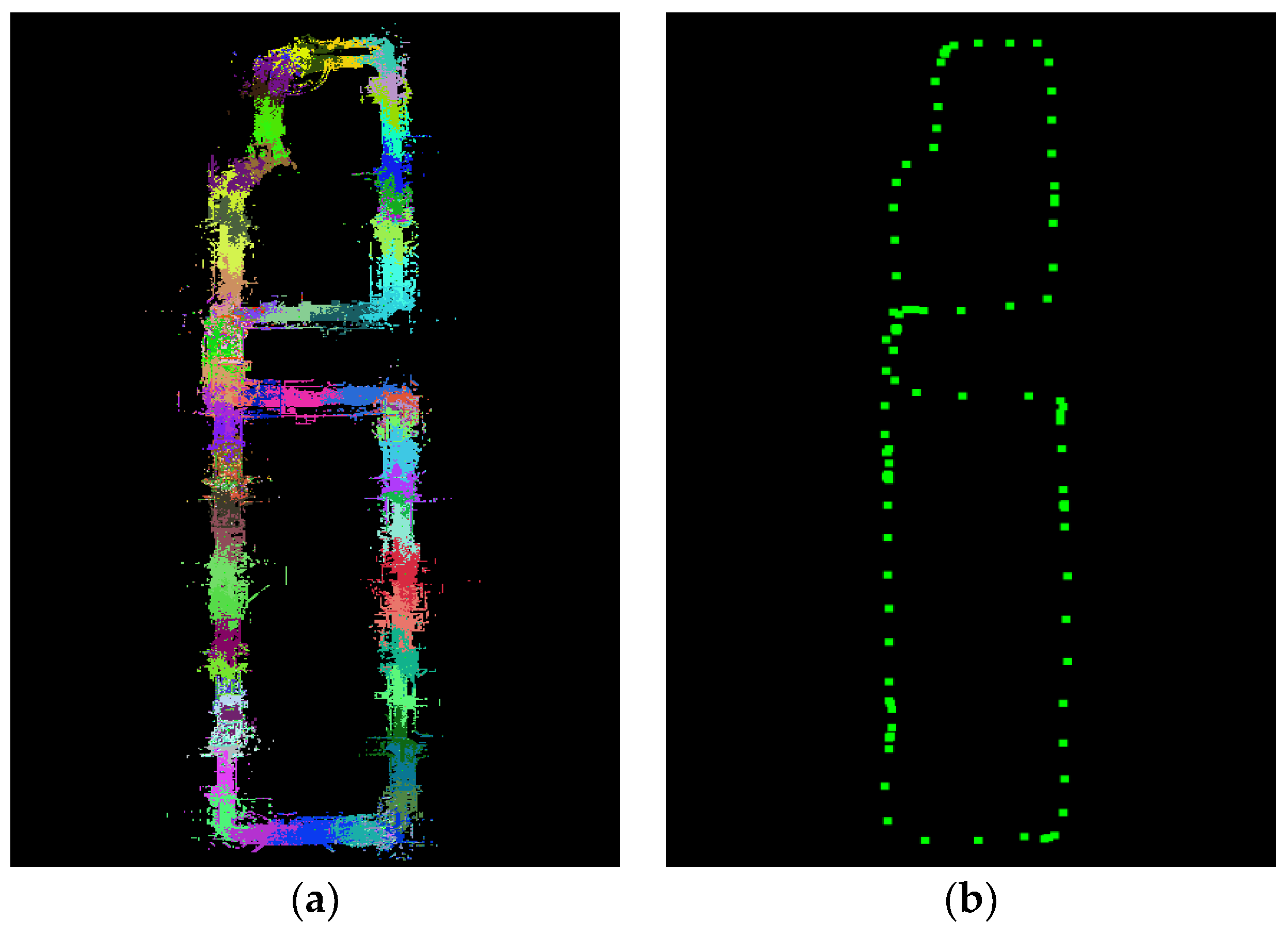
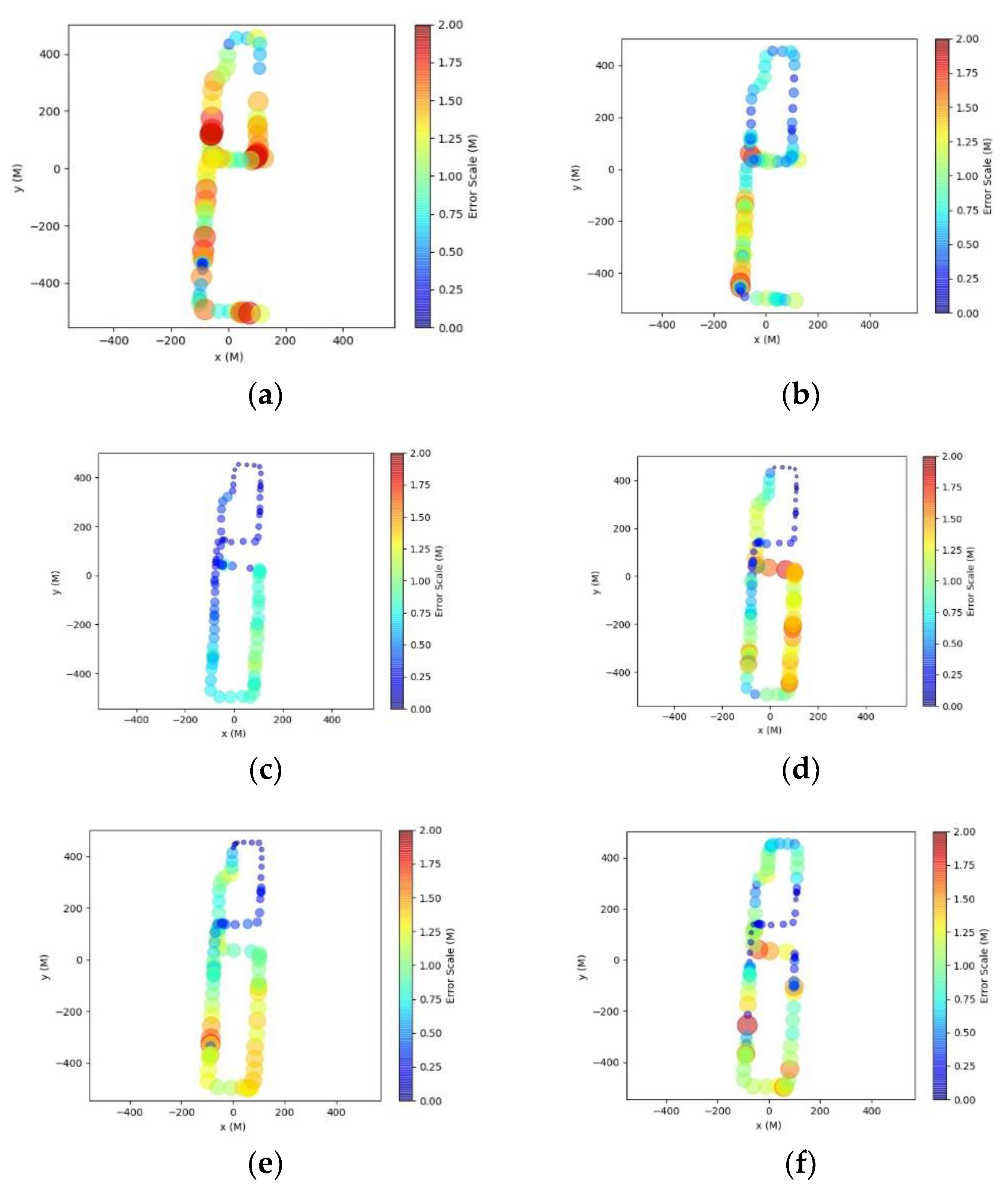
For a better visualization of the accuracy assessment results, Figure 6 shows color maps of the error values for the six point clouds and 5 s slice size length. Both color and the size of the data markers indicate the error magnitude for each slice. The points are plotted at the centroid of each individual slice (c.f. Figure 5b). In general, the navigation accuracy of a mobile mapping system changes slowly at different points in time. 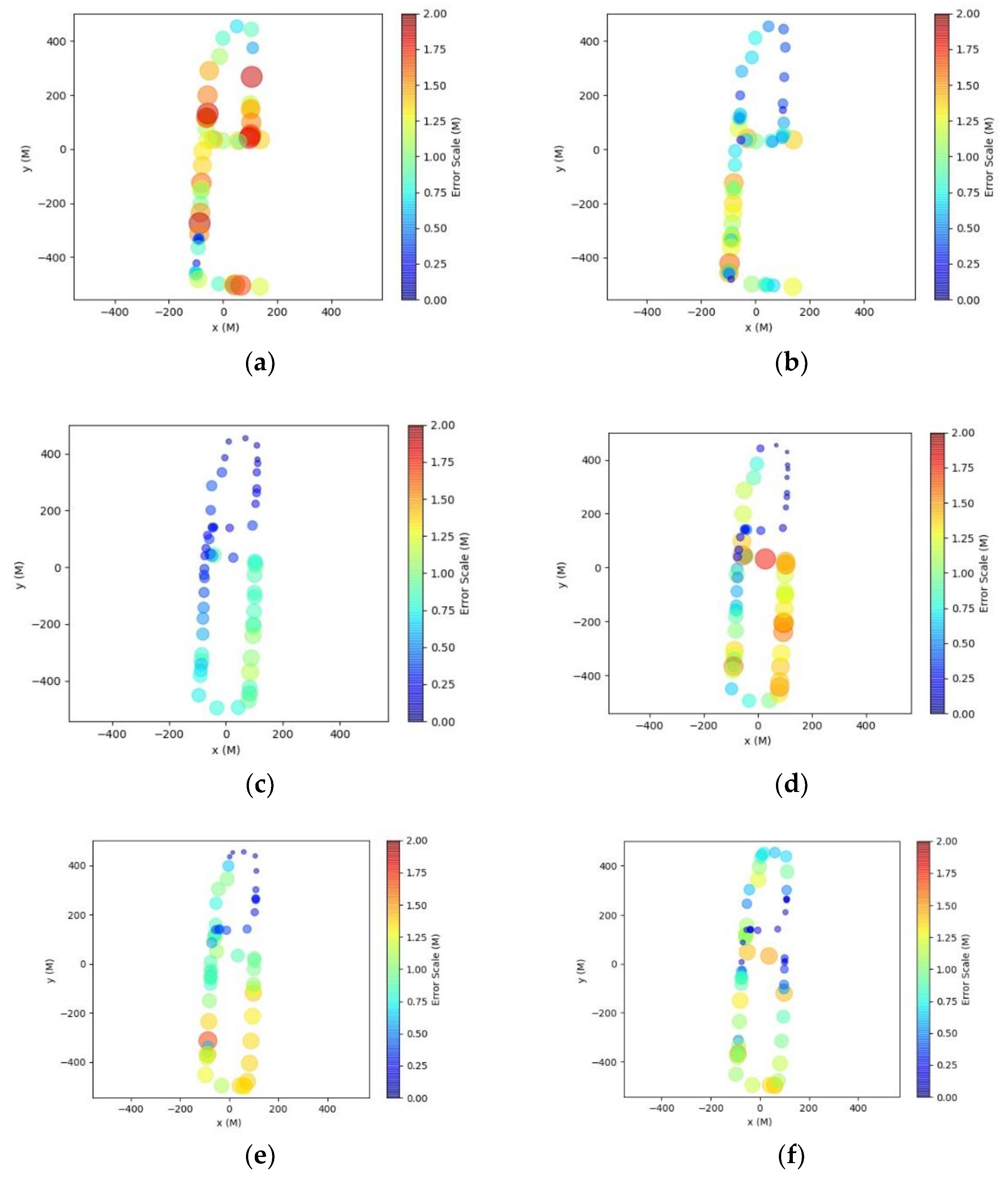Except for the InvenSense sensor, which is a lower grade of MEMS IMU, a smooth transition of error values from one slice to the next is generally evident, as can be seen in Figure 6. Similar observations are valid for experiments with slice size of 10 s (Figure 7). However, it was observed during testing that the smaller the slice size produced better the alignment following the registration. Accordingly, the accuracy assessment results from the 5 s slices are assumed as the more representative of the accuracy for the three sensors.

Multiple datasets were captured on separate dates with both the Epson and Honeywell sensors. Inspection of the results in common areas of the test field (Figure 7) reveals overall consistency of the results for both. Some local differences in accuracy do exist, in the vicinity of x = 100 m and y = 0 m, for example. These can be attributed to different satellite visibility conditions, as can other localized accuracy differences that can be seen between different sensors. Comparison of Table 2 with the results in Table 3 and Table 4 reveals that the MMS errors as determined by the proposed method are largely due to the low-cost IMUs rather than the Velodyne data. In fact, the new accuracy assessment methodology provides slightly more optimistic results than what is indicated by the trajectory difference statistics.

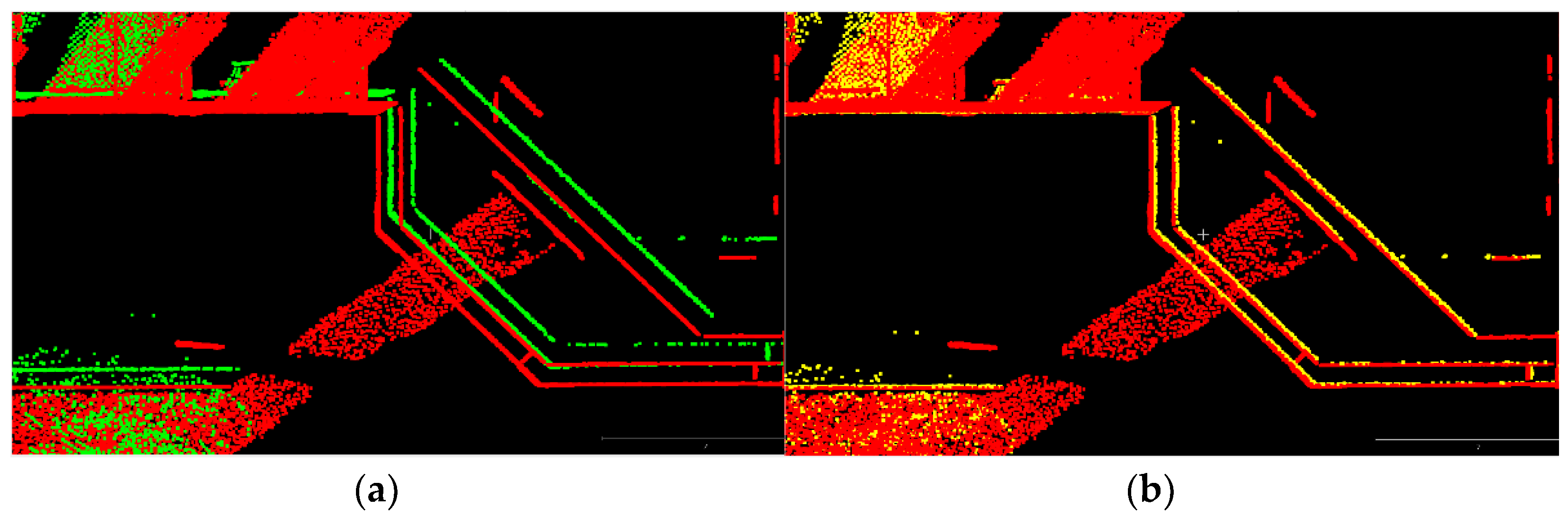
Further demonstration of the performance of the proposed method is given in Figure 8. This figure shows an example of point cloud cross-sections before and after registration. As can be seen, the ICP method provided precise alignment between the kinematic and static point clouds following the registration, even for point clouds that were significantly (~1 m) separated in three dimensions. This provides high confidence in the results of the proposed accuracy assessment methodology.

5. Conclusions

The evaluation of the metric performance of lightweight laser scanning systems utilized in MMSs, as well with on other platforms like UAVs, is of great importance given the growth of lightweight scanner and low-cost MEMS sensor usage. A methodology to perform this evaluation has been proposed. At its core is a large scale and rigorously surveyed test field situated in an urban environment. MMS point cloud data are decomposed into slices of short temporal duration and compared with the test field reference point cloud via ICP registration to quantify overall accuracy. The effectiveness of the method has been demonstrated on several Velodyne VLP-16 MMS datasets having different low-cost IMUs. The accuracy assessment is straightforward yet rigorous and gives a clear indication—both graphically and statistically—of overall point cloud quality along the MMS trajectory. Though not demonstrated here, it is expected that this method can be adapted for the assessment of lightweight laser scanners deployed on other platforms such as UAVs. Future work will focus on the investigation of real-time accuracy assessment of MMSs. Opportunity also exists to extend the testing to other types of navigation sensors and laser scanners.