Settlement and Bearing Capacity of Rectangular Footing in Reliance on the Pre-Overburden Pressure of Soil Foundation

Abstract

This article presents a solution for the quantitative evaluation of the stress–strain state (SSS) and the bearing capacity of rectangular foundations, factoring in the unit weight of the soil mass and different values of pre-overburden pressure (POP). In order to assess the SSS of the soil subgrade below a rigid rectangular footing under a uniformly distributed load, the authors applied the Boussinesq basic solution for an elastic half-space subjected to a vertical point load on its surface. As a result, the formulas for vertical stress, mean stress, shear strain, and volumetric strain for any point in Cartesian coordinates (x, y, z) and foundation settlement were determined. Additionally, the application of Hencky’s system of physical equations, with non-linear dependencies between mean stress and volumetric strain as well as deviator stress and shear strain, along with the experimental curves, depicts the relationships between bulk modulus and volume stress, and shear modulus and shear stress. The authors point out the non-linear behavior of the subgrade soil and propose a method for estimating the bearing capacity of a rigid rectangular foundation.

1. Introduction

The solutions for the problem of settlement of rigid rectangular footings have been proposed by a variety of authors [1,2,3,4,5,6] with various approaches. However, the limitation of which is a lack of explanation for the failure mechanism of soil medium underneath a rigid rectangular footing. By considering the vertical displacement as a result of components due to shear strain and volumetric strain of a loaded soil element, the authors denote not only the non-linear dependence between applied load and strain components but also the approach to the bearing capacity of rigid rectangular footings. To calculate shear strain and volumetric strain, the elastic–perfectly plastic model of Timoshenko [7] and the non-linear model proposed by Grigoryan are applied to indicate the non-linear behavior of the soil subgrade below a rectangular footing subjected to a uniformly distributed load, thereby achieving a dependency of deformation on load with a double curvature. So far, the non-linear analysis of soil subgrade under a rectangular foundation has solely been conducted using the finite element method. Therefore, it is essential to consider the non-linear soil deformation properties in analytical solutions based on the results from compression and triaxial tests. As a result, the varying values of shear modulus and bulk modulus depending on the deviator stress are elucidated clearly at any point in Cartesian coordinates. In addition, linear behavior can also be observed in the non-linear solution, when considering the shear modulus and bulk modulus as constant values. Consequently, the non-linear analysis turns out to be a classic linear analysis, based on Hooke’s law (G = const and K = const).

In this article, for the purpose of estimating the settlement and bearing capacity, we applied Hencky’s system of equations, which enables engineers to consider both linear and non-linear behaviors of soil media under a rectangular footing as well as to thoroughly separate the total vertical strain ${\epsilon }_{\mathrm{z}}$ into shear strain ${\epsilon }_{\gamma }$ and volumetric strain ${\epsilon }_{\mathrm{v}}$ as follows:

$${\epsilon }_{\mathrm{z}}={\epsilon }_{\gamma }+{\epsilon }_{\mathrm{v}}=\frac{{\sigma }_z-{\sigma }_{\mathrm{m}}}{G\left({\sigma }_{\mathrm{m}},{\tau }_{\mathrm{i}}/{\tau }_{\mathrm{i}}^{\ast }\right)}+\frac{{\sigma }_{\mathrm{m}}}{K\left({\sigma }_{\mathrm{m}}\right)}$$

(1)

in which $G\left({\sigma }_{\mathrm{m}},{\tau }_{\mathrm{i}}/{\tau }_{\mathrm{i}}^{\ast }\right)$ and $K\left({\sigma }_{\mathrm{m}}\right)$ are, respectively, shear modulus and bulk modulus, the values of which are relevant to the mean stress ${\sigma }_{\mathrm{m}}$ as well as the ratio of mobilized shear stress ${\tau }_{\mathrm{i}}$ to maximum shear stress ${\tau }_{\mathrm{i}}^{\ast }$, which can be found using the Mohr–Coulomb criterion at the considered points.

In a particular case, when G = const and K = const, Equation (1) turns into the Hooke’s law equation [8] that is presented as:

$${\epsilon }_{\mathrm{z}}=\frac{{\sigma }_{\mathrm{z}}-{\sigma }_{\mathrm{m}}}{2G}+\frac{{\sigma }_{\mathrm{m}}}{K}$$

(2)

$G\left({\sigma }_{\mathrm{m}},{\tau }_{\mathrm{i}}/{\tau }_{\mathrm{i}}^{\ast }\right)$ and $K\left({\sigma }_{\mathrm{m}}\right)$ can be retrieved from standard triaxial tests, the general view of which is observed in Figure 1 below.

A significant advantage of using Hencky’s system of equations is that it allows for the determination of the typical characteristics of total strain, volume, and shear strain of loaded soil elements. Figure 1 accurately depicts real soil behavior, with a decaying dependency between volumetric strain and mean stress, and a persistent dependency between shear strain and deviator stress. The final state following the latter dependency leads soil elements to failure. In other words, the progression of shear strain due to the increment of deviator stress induces an unlimited increase in the vertical deformation of soil samples in triaxial tests and the appearance of failure surfaces in the soil subgrade under rectangular and strip footings, while the volumetric strain is solely increased to stable values. This means that the volume or the porosity of soil elements will reach constant values when the critical state is achieved.

2. Methods and Analysis

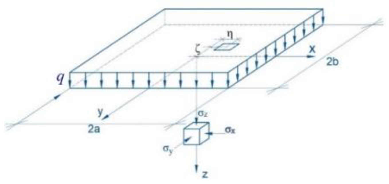
2.1. Theoretical Basics for Predicting the Settlement of a Rectangular Foundation in a Linear Formulation

As a computational geo-mechanical model for describing the stress state, a linearly deformable half-space under the influence of a constantly concentrated load q is considered, calculation schema of which is depicted in Figure 2. According to Boussinesq [9], the equations for the Cartesian normal stress and the mean stress are presented as follows:

$${\sigma }_{\mathrm{p}.\mathrm{z}}(x,y,z)=\frac{3q}{2\pi }\frac{z^3}{R^5}$$

(3)

$${\sigma }_{\mathrm{p}.\mathrm{m}}(x,y,z)=\frac{q}{3\pi }\left(1+\nu \right)\frac{z}{\sqrt{{\left(x^2+y^2+z^2\right)}^3}}$$

(4)

$${\sigma }_{\mathrm{p}.\mathrm{x}}=\frac{q}{2}\left[\frac{3x^{2}z}{R^5}-\left(1-2\nu \right)\left(\frac{x^2-y^2}{\left(x^2+y^2\right)R\left(z+R\right)}+\frac{y^{2}z}{\left(x^2+y^2\right)R^3}\right)\right]$$

(5)

$${\sigma }_{\mathrm{p}.\mathrm{y}}=\frac{q}{2}\left[\frac{3y^{2}z}{R^5}-\left(1-2\nu \right)\left(\frac{y^2-x^2}{\left(x^2+y^2\right)R\left(z+R\right)}+\frac{x^{2}z}{\left(x^2+y^2\right)R^3}\right)\right]$$

(6)

in which $R=\sqrt{\left(x^2+y^2+z^2\right)}$.

Based on Figure 3, in order to determine the distribution of all the stresses above at a depth beneath a rectangular footing, integrations Figure of expressions (3), (4), (5), and (6) with respect to $\eta$ (from −a to a) and $\xi$ (from −b to b) are carried out. However, in order to optimize the analytical calculations, the authors propose solely integrating Equations (3) and (4). The results are denoted as the following:

$$\begin{array}{l}{\sigma }_{\mathrm{z}}\left(x,y,z\right)=\frac{3q{z}^3}{2\pi }{\displaystyle \underset{-a}{\overset{a}{\int }}{\displaystyle \underset{-b}{\overset{b}{\int }}\frac{d\eta d\xi }{\sqrt{{\left({\left(x-\eta \right)}^2+{\left(y-\xi \right)}^2+z^2\right)}^5}}}}=\\ =\frac{q}{2\pi }\{\mathrm{arctg}\left[\frac{\left(x-a\right)\left(y-b\right)}{z\sqrt{{\left(x-a\right)}^2+{\left(y-b\right)}^2+z^2}}\right]+\mathrm{arctg}\left[\frac{\left(x+a\right)\left(y+b\right)}{z\sqrt{{\left(x+a\right)}^2+{\left(y+b\right)}^2+z^2}}\right]-\\ -\mathrm{arctg}\left[\frac{\left(x-a\right)\left(y+b\right)}{z\sqrt{{\left(x-a\right)}^2+{\left(y+b\right)}^2+z^2}}\right]-\mathrm{arctg}\left[\frac{\left(x+a\right)\left(y-b\right)}{z\sqrt{{\left(x+a\right)}^2+{\left(y-b\right)}^2+z^2}}\right]\}\\ +\frac{q}{2\pi }\{\frac{z\left(x+a\right)\left(y+b\right)\left[{\left(x+a\right)}^2+{\left(y+b\right)}^2+2z^2\right]}{\left[{\left(x+a\right)}^2+z^2\right]\left[{\left(y+b\right)}^2+z^2\right]\sqrt{{\left(x+a\right)}^2+{\left(y+b\right)}^2+z^2}}-\\ -\frac{z\left(x+a\right)\left(y-b\right)\left[{\left(x+a\right)}^2+{\left(y-b\right)}^2+2z^2\right]}{\left[{\left(x+a\right)}^2+z^2\right]\left[{\left(y-b\right)}^2+z^2\right]\sqrt{{\left(x+a\right)}^2+{\left(y-b\right)}^2+z^2}}+\\ +\frac{z\left(x-a\right)\left(y-b\right)\left[{\left(x-a\right)}^2+{\left(y-b\right)}^2+2z^2\right]}{\left[{\left(x-a\right)}^2+z^2\right]\left[{\left(y-b\right)}^2+z^2\right]\sqrt{{\left(x-a\right)}^2+{\left(y-b\right)}^2+z^2}}-\\ -\frac{z\left(x-a\right)\left(y+b\right)\left[{\left(x-a\right)}^2+{\left(y+b\right)}^2+2z^2\right]}{\left[{\left(x-a\right)}^2+z^2\right]\left[{\left(y+b\right)}^2+z^2\right]\sqrt{{\left(x-a\right)}^2+{\left(y+b\right)}^2+z^2}}\}\end{array}$$

(7)

$$\begin{array}{l}{\sigma }_{\mathrm{m}}\left(x,y,z\right)=\frac{qz}{3\pi }\left(1+\nu \right){\displaystyle {\int }_{-a}^a{\displaystyle {\int }_{-b}^b\frac{d\eta d\xi }{\sqrt{{\left({\left(x-\eta \right)}^2+{\left(y-\xi \right)}^2+z^2\right)}^3}}}}\\ =\frac{q\left(1+\nu \right)}{3\pi }\{\mathrm{arctg}\left[\frac{\left(x-a\right)\left(y-b\right)}{z\sqrt{{\left(x-a\right)}^2+{\left(y-b\right)}^2+z^2}}\right]+\mathrm{arctg}\left[\frac{\left(x+a\right)\left(y+b\right)}{z\sqrt{{\left(x+a\right)}^2+{\left(y+b\right)}^2+z^2}}\right]-\\ -\mathrm{arctg}\left[\frac{\left(x-a\right)\left(y+b\right)}{z\sqrt{{\left(x-a\right)}^2+{\left(y+b\right)}^2+z^2}}\right]-\mathrm{arctg}\left[\frac{\left(x+a\right)\left(y-b\right)}{z\sqrt{{\left(x+a\right)}^2+{\left(y-b\right)}^2+z^2}}\right]\}\end{array}$$

(8)

While considering the obtained expressions (7) and (8) on the vertical axis z (x = 0; y = 0), their brief forms can be expressed as follows:

$${\sigma }_{\mathrm{z}}=\frac{2q}{\pi }\left[\mathrm{arctg}\frac{ab}{z\sqrt{a^2+b^2+z^2}}+\frac{abz\left(a^2+b^2+2z^2\right)}{\left(a^2+z^2\right)\left(b^2+z^2\right)\sqrt{a^2+b^2+z^2}}\right]$$

(9)

$${\sigma }_{\mathrm{m}}=\frac{4q\left(1+\nu \right)}{3\pi }\left[\mathrm{arctg}\left(\frac{ab}{z\sqrt{a^2+b^2+z^2}}\right)\right]$$

(10)

Under the generalized Hooke’s Law, the total strain ${\epsilon }_{\mathrm{z}}$ of a soil element can be considered through two components, volumetric strain ${\epsilon }_{\mathrm{v}}$ and shear strain ${\epsilon }_{\gamma }$, which are dependent on vertical stress, mean stress, and the stiffness of the soil.

$${\epsilon }_{\mathrm{z}}={\epsilon }_{\mathsf{\gamma }}+{\epsilon }_{\mathrm{v}}=\frac{{\sigma }_z-{\sigma }_{\mathrm{m}}}{2G}+\frac{{\sigma }_{\mathrm{m}}}{K}$$

(11)

The obtained expressions above reveal that, for the linear elastic soil medium, the shear strain and volumetric strain of soil elements at any point in Cartesian coordinates (x, y, z) can be determined using expressions of ${\sigma }_{\mathrm{z}}$ and ${\sigma }_{\mathrm{m}}$ along with the stiffness parameters. In the particular case of a rigid rectangular footing, in order to evaluate its settlement, the expression (11) requires an integration with respect to z (from 0 to H, where H is the depth of the compressed thickness of the soil massif under the footing). Therefore, the total settlement is presented as follows:

$$S=S_{\gamma }+S_{\mathrm{v}}={\displaystyle \underset{0}{\overset{H}{\int }}{\mathsf{\epsilon }}_{\mathsf{\gamma }}d\mathrm{z}+}{\displaystyle \underset{0}{\overset{H}{\int }}{\epsilon }_{\mathrm{v}}d\mathrm{z}}={\displaystyle \underset{0}{\overset{H}{\int }}\frac{{\sigma }_z-{\sigma }_{\mathrm{m}}}{2G}d\mathrm{z}+}{\displaystyle \underset{0}{\overset{H}{\int }}\frac{{\sigma }_{\mathrm{m}}}{K}}d\mathrm{z}$$

(12)

in which $S_{\gamma }$ and $S_{\mathrm{v}}$ are the values of settlement due to shear strain and volumetric strain, respectively.

For the purpose of convenience, the authors propose an analytical method of total settlement assessment using expressions of ${\sigma }_{\mathrm{z}}$ and ${\sigma }_{\mathrm{m}}$ on the axis that passes through the center (0, 0, 0) of a rigid rectangular footing. The expressions of $S_{\gamma }$ and $S_{\mathrm{v}}$ are illustrated as:

$$S_{\mathsf{\gamma }}={\displaystyle \underset{0}{\overset{H}{\int }}\frac{{\sigma }_z-{\sigma }_{\mathrm{m}}}{2G}d\mathrm{z}=}{\displaystyle \underset{0}{\overset{H}{\int }}\left[\frac{q\left(1-2\nu \right)}{3\pi G}\mathrm{arctg}\frac{ab}{z\sqrt{a^2+b^2+z^2}}+\frac{q}{\pi G}\frac{abz\left(a^2+b^2+2z^2\right)}{\left(a^2+z^2\right)\left(b^2+z^2\right)\sqrt{a^2+b^2+z^2}}\right]}\mathrm{d}z$$

(13)

$$S_{\mathrm{v}}={\displaystyle \underset{0}{\overset{H}{\int }}\frac{{\sigma }_{\mathrm{m}}}{K}}d\mathrm{z}=\frac{4q\left(1+\nu \right)}{3\pi K}{\displaystyle \underset{0}{\overset{H}{\int }}\mathrm{arctg}\left(\frac{ab}{z\sqrt{a^2+b^2+z^2}}\right)}\mathrm{d}z$$

(14)

The analyzed expression of settlement $S_{\mathsf{\gamma }}$ due to shear strain consists of three components A B C as follows:

$$S_{\mathsf{\gamma }}=A+B+C$$

(15)

in which

$$A=\frac{q\left(1-2\nu \right)}{3\pi G}h \mathrm{arctg}\frac{ab}{h_{}\sqrt{a^2+b^2+h^2}}$$

(16)

$$\begin{array}{l}B=\frac{q\left(1-2\nu \right)}{3\pi G}\{H_1\ln \left|\frac{8H_1^3-2\left(a^2+b^2\right)H_1+ab\sqrt{a^2+b^2+h_{}{}^2}}{-8H_1^3+2\left(a^2+b^2\right)H_1+ab\sqrt{a^2+b^2+h_{}{}^2}}\right|\\ +H_2\ln \left|\frac{8H_2^3-2\left(a^2+b^2\right)H_2+ab\sqrt{a^2+b^2+h_{}{}^2}}{-8H_2^3+2\left(a^2+b^2\right)H_2+ab\sqrt{a^2+b^2+h_{}{}^2}}\right|\\ -H_1\ln \left|\frac{8H_1^3-2\left(a^2+b^2\right)H_1+ab\sqrt{a^2+b^2}}{-8H_1^3+2\left(a^2+b^2\right)H_1+ab\sqrt{a^2+b^2}}\right|\\ -H_2\ln \left|\frac{8H_2^3-2\left(a^2+b^2\right)H_2+ab\sqrt{a^2+b^2}}{-8H_2^3+2\left(a^2+b^2\right)H_2+ab\sqrt{a^2+b^2}}\right|\}\end{array}$$

(17)

$$\begin{array}{l}C=\frac{q}{2\pi G}[a\ln \left|\frac{\sqrt{a^2+b^2+h_{}{}^2}-b}{\sqrt{a^2+b^2+h_{}{}^2}+b}\right|-a\ln \left|\frac{\sqrt{a^2+b^2}-b}{\sqrt{a^2+b^2}+b}\right|+\\ +b\ln \left|\frac{\sqrt{a^2+b^2+h_{}{}^2}-a}{\sqrt{a^2+b^2+h_{}{}^2}+a}\right||-b\ln \left|\frac{\sqrt{a^2+b^2}-a}{\sqrt{a^2+b^2}+a}\right||]\end{array}$$

(18)

$$H_1=\sqrt{\frac{\left(a^2+b^2\right)-\sqrt{{\left(a^2+b^2\right)}^2-4a^2{b}^2}}{8}};H_2=\sqrt{\frac{\left(a^2+b^2\right)+\sqrt{{\left(a^2+b^2\right)}^2-4a^2{b}^2}}{8}}$$

(19)

The settlement $S_{\mathrm{v}}$ due to the volumetric strain caused by mean stress can be procured by analyzing expression (12) with the form of:

$$\begin{array}{l}{S}_{\mathrm{v}}=\frac{4q\left(1+\nu \right)}{3\pi K}h\mathrm{arctg}\frac{ab}{h\sqrt{a^2+b^2+h^2}}+\\ +\frac{4q\left(1+\nu \right)}{3\pi K}{H}_1\ln \left|\frac{8H_1^3-2\left(a^2+b^2\right)H_1+ab\sqrt{a^2+b^2+h^2}}{-8H_1^3+2\left(a^2+b^2\right)H_1+ab\sqrt{a^2+b^2+h^2}}\right|\\ -\frac{4q\left(1+\nu \right)}{3\pi K}{H}_1\ln \left|\frac{8H_1^3-2\left(a^2+b^2\right)H_1+ab\sqrt{a^2+b^2}}{-8H_1^3+2\left(a^2+b^2\right)H_1+ab\sqrt{a^2+b^2}}\right|+\\ +\frac{4q\left(1+\nu \right)}{3\pi K}{H}_2\ln \left|\frac{8H_2^3-2\left(a^2+b^2\right)H_2+ab\sqrt{a^2+b^2+h^2}}{-8H_2^3+2\left(a^2+b^2\right)H_2+ab\sqrt{a^2+b^2+h^2}}\right|-\\ -\frac{4q\left(1+\nu \right)}{3\pi K}{H}_2\ln \left|\frac{8H_2^3-2\left(a^2+b^2\right)H_2+ab\sqrt{a^2+b^2}}{-8H_2^3+2\left(a^2+b^2\right)H_2+ab\sqrt{a^2+b^2}}\right|\end{array}$$

(20)

Considering the example with the following inputs: q₁ = 1000 kPa; a₁ = 0.5 m; b₁ = 1.5 m; ${\nu }_1$ = 0.3; H₁ = 20 m; G₁ = 10,000 kPa; K₁ = 65,000 kPa; q₂ = 1500 kPa; a₂ = 1.5 m; b₂ = 3 m; ${\nu }_2$ = 0.3; H₂ = 25 m; G₂ = 15,000 kPa; K₂ = 97,500 kPa; q₃ = 1500 kPa; a₃ = 2 m; b₃ = 4 m; ${\nu }_3$ = 0.3; H₃ = 30 m; G₃ = 20,000 kPa; and K₃ = 130,000 kPa. By using math software for engineering calculations (Mathcad), we obtain: $S_{\mathsf{\gamma }1}$ = 0.06105 m; $S_{\mathrm{v}1}$ = 0.01436 m; $S_{\mathsf{\gamma }2}$ = 0.1180 m; $S_{\mathrm{v}2}$ = 0.02911 m; $S_{\mathsf{\gamma }3}$ = 0.1556 m; and $S_{\mathrm{v}3}$ = 0.03859 m. It is substantially important to note that the values of $S_{\mathsf{\gamma }1}$, $S_{\mathsf{\gamma }2}$, and $S_{\mathsf{\gamma }3}$ are 4.25, 4.06, and 4.032 times higher than the values of $S_{\mathrm{v}1}$, $S_{\mathsf{\gamma }2}$, and $S_{\mathrm{v}3}$ ($S_{\mathsf{\gamma }1}=4.25S_{\mathrm{v}1}$; $S_{\mathsf{\gamma }2}=4.06S_{\mathrm{v}2}$; $S_{\mathsf{\gamma }3}=4.032S_{\mathrm{v}3}$), respectively. Thus, it can be concluded that in linear elastic half-space, the settlement of a loaded soil subgrade mainly occurs due to the shear strain, which is over 80% of the total value, while nearly 20% of the total value comes from the volume change. The distributions of shear strain ${\epsilon }_{\mathsf{\gamma }}(z)$ and volumetric strain ${\epsilon }_v(z)$, calculated using expression (11), with a depth corresponding to the first group of parameters (q₁, a₁, b₁, ${\nu }_1$, H₁, G₁, K₁) are illustrated in Figure 4 and Figure 5.

As presented in expression (11), the shear ${\epsilon }_{\mathsf{\gamma }}(z)$ and volumetric strains ${\epsilon }_v(z)$ are calculated through the deviator stress ${\sigma }_z-{\sigma }_{\mathrm{m}}$ and volumetric stress ${\sigma }_{\mathrm{m}}$, which are derived from expressions (7) and (8). As a result, the variation of ${\epsilon }_{\mathsf{\gamma }}(z)$, and ${\epsilon }_v(z)$ with depth is accompanied by a change of ${\sigma }_z-{\sigma }_{\mathrm{m}}$ and ${\sigma }_{\mathrm{m}}$, respectively. Therefore, the decrease in values of ${\sigma }_z-{\sigma }_{\mathrm{m}}$ and ${\sigma }_{\mathrm{m}}$ as the depth increases leads to the dip in ${\epsilon }_{\mathsf{\gamma }}(z)$ and ${\epsilon }_v(z)$.

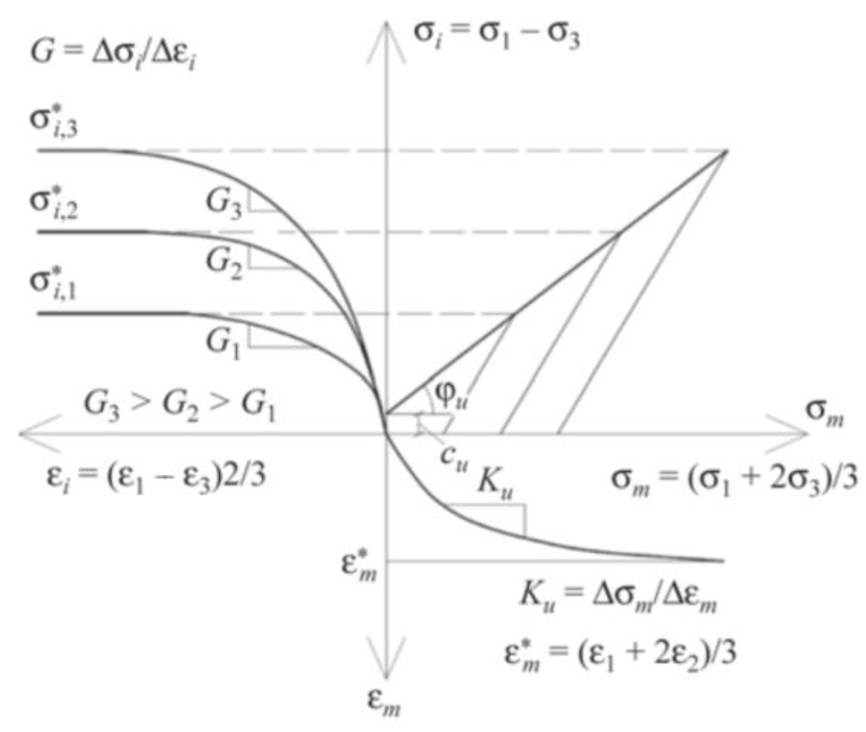
2.2. Hencky’s System of Physical Equations

Apart from the solution for the linear relationships above, the usage of Hencky’s system of physical equations [10] allows modeling of non-linear relationships between stress and strain (see also [11]), which are mathematically described as follows:

$$\begin{array}{l}{\epsilon }_{\mathrm{x}}=\chi \left({\sigma }_{\mathrm{x}}-{\sigma }_{\mathrm{m}}\right)+{\chi }^{\ast }{\sigma }_{\mathrm{m}}{;}_{}{\epsilon }_{\mathsf{\gamma }.}{}_{\mathrm{xy}}=2\chi .{\tau }_{\mathrm{xy}}\\ {\epsilon }_{\mathrm{y}}=\chi \left({\sigma }_{\mathrm{y}}-{\sigma }_{\mathrm{m}}\right)+{\chi }^{\ast }{\sigma }_{\mathrm{m}}{;}_{}{\epsilon }_{\mathsf{\gamma }.}{}_{\mathrm{yz}}=2\chi .{\tau }_{\mathrm{yz}}\\ {\epsilon }_{\mathrm{z}}=\chi \left({\sigma }_{\mathrm{z}}-{\sigma }_{\mathrm{m}}\right)+{\chi }^{\ast }{\sigma }_{\mathrm{m}}{;}_{}{\epsilon }_{\mathsf{\gamma }.}{}_{\mathrm{zy}}=2\chi .{\tau }_{\mathrm{zy}}\end{array}$$

(21)

in which

$$\chi =\frac{{\gamma }_{\mathrm{i}}}{2{\tau }_{\mathrm{i}}}=\frac{f\left({\tau }_{\mathrm{i}},{\sigma }_{\mathrm{m}},{\mu }_{\sigma }\right)}{2{\tau }_{\mathrm{i}}}\mathrm{and}{\chi }^{\ast }=\frac{{\epsilon }_{\mathrm{m}}}{{\sigma }_{\mathrm{m}}}=\frac{f\left({\tau }_{\mathrm{i}},{\sigma }_{\mathrm{m}},{\mu }_{\sigma }\right)}{{\sigma }_{\mathrm{m}}}$$

(22)

${\tau }_{\mathrm{i}}$ is the value of current shear stress of a loaded soil element and ${\mu }_{\sigma }$ is the Lode–Nadai coefficient, which characterizes the forms of the stress state.

It is noted that, when $\chi$ and ${\chi }^{\ast }$ take the forms of $\raisebox{1ex}{$1$}\!\left/ \!\raisebox{-1ex}{$2G$}\right.$ and $\raisebox{1ex}{$1$}\!\left/ \!\raisebox{-1ex}{$K$}\right.$, respectively, Hencky’s system of physical equations turns into the Hooke’s law formulas for soil elements, in which $G=\raisebox{1ex}{$E$}\!\left/ \!\raisebox{-1ex}{$2\left(1+\nu \right)$}\right.$ and $K=\raisebox{1ex}{$E$}\!\left/ \!\raisebox{-1ex}{$\left(1-2\nu \right)$}\right.$ are applied as the primary stiffness parameters.

In order to model the non-linear relationship between the volumetric strain and mean stress of loaded soil elements, we used an exponential function dependency proposed by Grigoryan [12]. Its form is as follows:

$${\epsilon }_{\mathrm{m}}\left({\sigma }_{\mathrm{m}}\right)={\epsilon }^{\ast }\left(1-e^{-\alpha {\sigma }_{\mathrm{m}}}\right)$$

(23)

where ${\epsilon }^{\ast }$ is the limiting value of volumetric deformation, ${\epsilon }_{\mathrm{m}}\left({\sigma }_{\mathrm{m}}\right)$ is the average volumetric deformation with varying values depending on mean stress ${\sigma }_{\mathrm{m}}$, and $\alpha$ is a non-linearity parameter, which can be determined experimentally.

By considering the elementary definition of volume modulus observed by the ratio of volumetric strain to volume stress, the varying values of secant bulk modulus K, which depend on the stress state of the loaded soil elements, can be represented by the following form:

$$\begin{array}{l}\frac{{\epsilon }_{\mathrm{m}}}{{\sigma }_{\mathrm{m}}}=\frac{1}{K}=\frac{{\epsilon }^{\ast }\left(1-e^{-\alpha {\sigma }_{\mathrm{m}}}\right)}{{\sigma }_{\mathrm{m}}}\\ K=\frac{{\sigma }_{\mathrm{m}}}{{\epsilon }_{\mathrm{m}}}\end{array}$$

(24)

Being close to infinite, ${\epsilon }_{\mathrm{m}}$ will eventually reach ${\epsilon }^{\ast }$ when $\alpha =0$ and ${\epsilon }^{\ast }={\epsilon }_{\mathrm{m}}$, and expression (24) will have the form of Hooke’s law for linear elastic materials.

To express the elastic–plastic behaviors of soil elements subjected to shear stress, the formula proposed by Tymoshenko [13,14] can be applied.

$${\epsilon }_{\mathsf{\gamma }.}{}_i=\frac{{\tau }_{\mathrm{i}}}{G_{\mathrm{c}}^{\mathrm{e}}}\cdot \frac{{\tau }_{\mathrm{i}}^{\ast }}{{\tau }_{\mathrm{i}}^{\ast }-{\tau }_{\mathrm{i}}}$$

(25)

where ${\tau }_{\mathrm{i}}^{\ast }$ is the maximum value of shear stress, which is calculated by the following equation:

$${\tau }_{\mathrm{i}}^{\ast }=\left({\sigma }_{\mathrm{m}}+{\sigma }_{\mathrm{g}}\right)\cdot tg{\varphi }_{\mathrm{i}}+c_{\mathrm{i}}$$

(26)

in which ${\sigma }_{\mathrm{m}}$ is the mean stress of loaded soil elements; ${\varphi }_{\mathrm{i}}$ and $c_{\mathrm{i}}$ are the angle of internal friction and the cohesive strength, respectively, determined by the Mohr diagram and failure envelopes; and ${\sigma }_{\mathrm{g}}$ is the vertical earth pressure, which in the condition of normally consolidated soil is represented by the form:

$${\sigma }_{\mathrm{g}}=\gamma h$$

(27)

where $\gamma$ is the unit weight of soil and h is the depth at which ${\tau }_{\mathrm{i}}^{\ast }$ is estimated.

In the case of over-consolidated soil with the maximum effective vertical overburden stress that the soil element has sustained in the past, the formula of ${\sigma }_{\mathrm{g}}$ takes the following form:

$${\sigma }_{\mathrm{g}}^{\prime }=\gamma h+{\sigma }_{\mathrm{P}}$$

(28)

where ${\sigma }_{\mathrm{P}}$ is pre-overburden pressure, which can be determined through pre-consolidation pressure using Casagrande’s graphical method [15] based on the compression test results. The instructions for the method can be observed in the Russian Federation’s national standard on soils, under laboratory method for determining the over-consolidation characteristics. Equation (25) implies that:

$$G=G^e\left(1-\frac{{\tau }_{\mathrm{i}}}{{\tau }_{\mathrm{i}}^{\ast }}\right)$$

(29)

in which $G^e$ is the value of elastic shear modulus of the soil.

It follows from expression (29) that for ${\tau }_{\mathrm{i}}\to {\tau }_{\mathrm{i}}^{\ast }$, we procure $G\to 0$ and ${\epsilon }_{\mathsf{\gamma }.\mathrm{i}}\to \infty$. Figure 6a–c demonstrate respectively the colour shadings of mean stress ${\sigma }_{\mathrm{m}}$, vertical stress ${\sigma }_{\mathrm{z}}$, and deviator stress ${\sigma }_{\mathrm{z}}-{\sigma }_{\mathrm{m}}$ that are derived from Equations (7) and (8) in the XOZ-plane.

3. Results and Discussion

3.1. Calculation of Total Strain in Soil Layers Taking into Account the Non-Linear Deformability and Their Various Mechanical Parameters

Throughout this article, it has been emphasized that when estimating the settlement of a rectangular footing, Hencky’s system of physical equations prominently manifests its special feature of analyzing the total deformations as shear and volumetric strains, taking into consideration the varying values of soil stiffness parameters, which depends on the stress-state of the soil elements. The equation for total strain is briefly displayed as follows:

$${\epsilon }_{\mathrm{z}}={\epsilon }_{\mathsf{\gamma }}+{\epsilon }_v=\frac{{\sigma }_z-{\sigma }_{\mathrm{m}}}{G\left({\sigma }_{\mathrm{m}},{\tau }_{\mathrm{i}}/{\tau }_{\mathrm{i}}^{\ast }\right)}+\frac{{\sigma }_{\mathrm{m}}}{K\left({\sigma }_{\mathrm{m}}\right)}$$

(30)

Putting Equations (24) and (29) into the procured expression (30) above, we get:

$${\epsilon }_{\mathrm{z}}=\frac{{\sigma }_z-{\sigma }_{\mathrm{m}}}{2G^e\left(1-\frac{{\tau }_{\mathrm{i}}}{{\tau }_{\mathrm{i}}^{\ast }}\right)}+{\epsilon }^{\ast }\left(1-e^{-\alpha {\sigma }_{\mathrm{m}}}\right)$$

(31)

in which the definitions of $G^e$, ${\tau }_{\mathrm{i}}^{\ast }$, ${\epsilon }^{\ast }$, ${\sigma }_z$, and ${\sigma }_{\mathrm{m}}$ are detailed above.

According to [16], Mohr’s circle reveals that the maximum shear stress in soil elements takes a value that is equal to half of the difference between the maximum principal stress ${\sigma }_1$ and ${\sigma }_3$. On the axis that passes through the center (0, 0, 0) of a rigid rectangular footing, the vertical stress ${\sigma }_z$ and the two components ${\sigma }_x$ and ${\sigma }_y$ act as the principal stress ${\sigma }_1$, ${\sigma }_2$, and ${\sigma }_3$, respectively. Therefore, the value of shear stress that occurs in a cubic soil element ${\tau }_{\mathrm{i}}$ can be accepted as:

$${\tau }_i=\frac{{\sigma }_1-{\sigma }_3}{2}=\frac{{\sigma }_z-{\sigma }_x}{2}$$

(32)

where ${\sigma }_x$ is calculated by integrating ${\sigma }_{\mathrm{p}.x}$, which corresponds to the case of point load with respect to $\eta$ (from −a to a) and to $\xi$ (from −b to b).

$${\sigma }_x={\displaystyle \underset{-a}{\overset{a}{\int }}{\displaystyle \underset{-b}{\overset{b}{\int }}\frac{q}{2}\left[\frac{3{\left(x-\eta \right)}^{2}z}{R_1{}^5}-\left(1-2\nu \right)\left(\frac{{\left(x-\eta \right)}^2-{\left(y-\xi \right)}^2}{\left({\left(x-\eta \right)}^2+{\left(y-\xi \right)}^2\right)R_1\left(z+R_1\right)}+\frac{{\left(y-\xi \right)}^{2}z}{\left({\left(x-\eta \right)}^2+{\left(y-\xi \right)}^2\right)R_1{}^3}\right)\right]d\eta d\xi }}$$

(33)

$$R_1=\sqrt{{\left(x-\eta \right)}^2+{\left(y-\xi \right)}^2+z^2}$$

With a rigid square footing, thanks to its symmetrical shape, the stress–strain state (SSS) of the soil subgrade under the footing can be considered as the SSS of a soil sample in a symmetric triaxial test, in which ${\sigma }_3$ and ${\sigma }_2$ are the same. Therefore, the equation ${\tau }_i$ can be written in the following form (see also [17]):

$${\tau }_i=\frac{{\sigma }_z-{\sigma }_x}{2}=\frac{{\sigma }_z-\frac{3{\sigma }_{\mathrm{m}}-{\sigma }_z}{2}}{2}=\frac{3}{2}\left({\sigma }_z-{\sigma }_{\mathrm{m}}\right)$$

(34)

where ${\sigma }_z$ and ${\sigma }_{\mathrm{m}}$ are calculated by Equations (9) and (10).

From analysis of Equation (31), it can be concluded that the component deformations grow according to the loading increment. The curve of the shear strain ${\epsilon }_{\gamma }$ takes a parabolic form and has a tendency of infinity, while the progress of the volumetric strain ${\epsilon }_v$ tends to be dampened. As a sum of the two components ${\epsilon }_{\gamma }$ and ${\epsilon }_v$, the total strain of a loaded soil element possesses a double curvature and turns out to be infinite at ${\tau }_{\mathrm{i}}\to {\tau }_{\mathrm{i}}^{\ast }$. Dependency curves between shear strain, volumetric strain, total strain, and loading values with various values of stiffness and strength parameters can be observed using Equation (30). Figure 7 and Figure 8 indicate the PTC Mathcad results for Equation (31).

3.2. Calculation of Total Settlement of Soil Layers Taking into Account the Non-Linear Deformability and Their Various Mechanical Parameters

The dependency curve of total settlement S(q) on surface load q is derived by integrating Equation (31) with respect to z (from 0 to H, where H is the depth of the compressed thickness of the soil massif under the footing). This is represented as follows:

$$S(q)=S_{\mathsf{\gamma }}(q)+S_v(q)={\displaystyle \underset{0}{\overset{H}{\int }}\frac{{\sigma }_z(q)-{\sigma }_{\mathrm{m}}(q)}{2G^e\left[1-\frac{1}{2}\frac{{\sigma }_z(q)-{\sigma }_x(q)}{\left({\sigma }_{\mathrm{m}}(q)+\gamma h+{\sigma }_{\mathrm{P}}\right)\cdot tg\varphi +c}\right]}}d\mathrm{z}+{\displaystyle \underset{0}{\overset{H}{\int }}{\epsilon }^{\ast }\left(1-e^{-\alpha {\sigma }_{\mathrm{m}}(q)}\right)}d\mathrm{z}$$

(35)

in which $S_{\gamma }(q)$ and $S_v(q)$ are the shear and volume components, respectively, that are determined as follows:

$$S_{\mathsf{\gamma }}(q)={\displaystyle \underset{0}{\overset{H}{\int }}\frac{{\sigma }_z(q)-{\sigma }_{\mathrm{m}}(q)}{2G^e\left[1-\frac{1}{2}\frac{{\sigma }_z(q)-{\sigma }_x(q)}{\left({\sigma }_{\mathrm{m}}(q)+\gamma h+{\sigma }_{\mathrm{P}}\right) \cdot tg\varphi +c}\right]}}d\mathrm{z}$$

(36)

$$S_v(q)={\displaystyle \underset{0}{\overset{H}{\int }}{\epsilon }^{\ast }\left(1-e^{-\alpha {\sigma }_{\mathrm{m}}(q)}\right)}d\mathrm{z}$$

(37)

Along with the increment in values of surface load q, the rise in settlement S(q) will arrive at an infinite value based on the strength parameters of the soil. The value of surface load q corresponding to the infinity state can be observed as the bearing capacity of the rigid rectangular footing. Figure 9 shows dependency plots for $S_{\mathsf{\gamma }}(q)-1$, $S_v(q)-1$, and $S(q)-3$, determined by Equation (35), while Figure 10 shows dependency plots for $S(q)$ at different values of pre-overburden pressure ${\sigma }_{\mathrm{P}}$, and Figure 10 demonstrates dependency plots for $S(q)$ at various values of foundation depth z.

4. Conclusions

• The settlement and bearing capacity of rectangular footings are regarded as the main calculation parameters when designing foundations used in construction.
• These calculations show that geo-mechanical models for foundation, including geometric parameters of the footing (length, width, depth, initial and boundary conditions) and computational soil models, such as linear and non-linear models with different systems of physical equations (Hooke and Hencky), have a significant influence on the evaluation of settlement and bearing capacity.
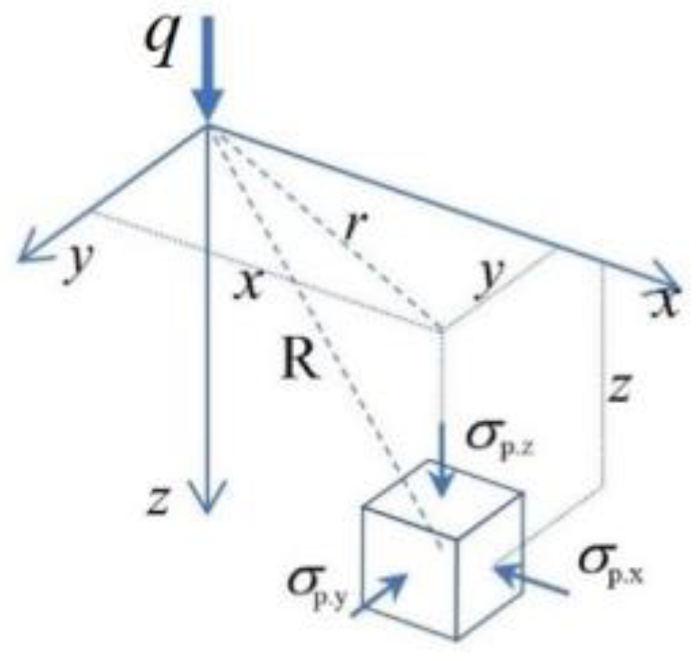
• The computational soil model used in this article, with the possibility of lateral expansion (${\epsilon }_x\ne 0$, and ${\epsilon }_{\mathrm{y}}\ne 0$), along with the elastic–plastic model for shear strain–stress dependency and the non-linear model for volumetric strain–stress dependency as parts of Hencky’s system of physical equations, allows us to present the total deformation as the sum of the volumetric and shear components (${\epsilon }_{\mathrm{z}}={\epsilon }_{\mathsf{\gamma }}+{\epsilon }_{\mathrm{v}}$). Only in this case do the strain–stress curve and the settlement–load curve both have decaying and persistent (double curvature) characteristics.
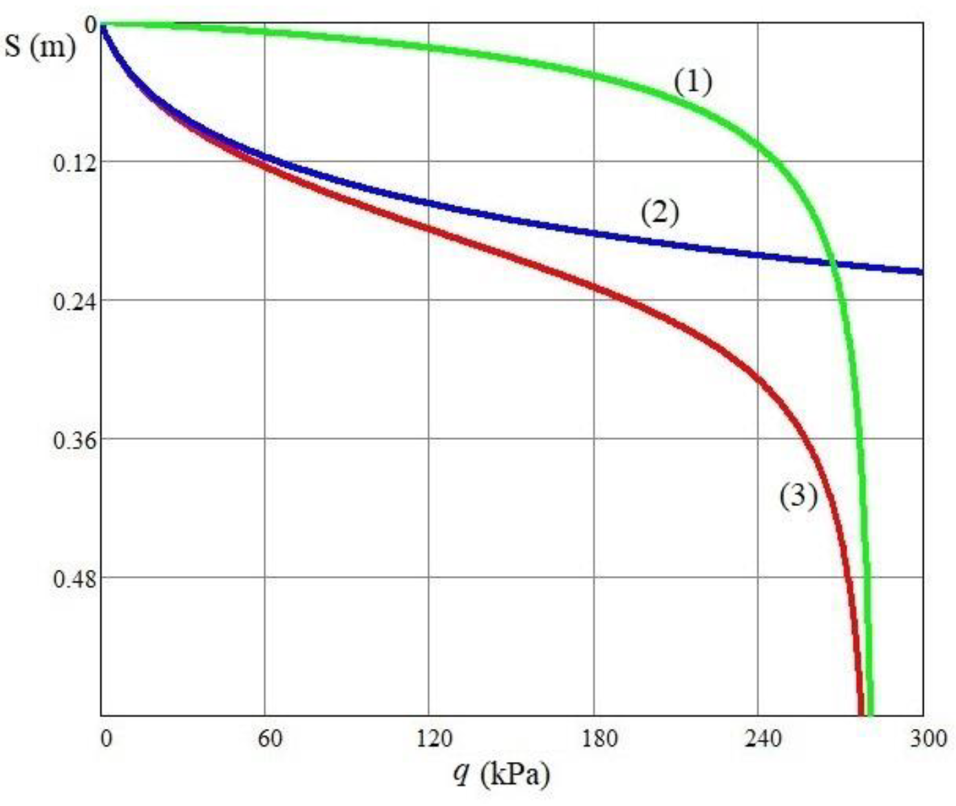
• The computational soil model proposed here indicates that, thanks to the choice of different combinations of stiffness (G^e, $\nu$, ${\epsilon }^{\ast }$, $\alpha$) and strength parameters (${\varphi }_{}$ and c), the curve of dependency between settlement and load can be observed as decaying or persistent with various bending degrees of the curvature.
• This article presents a substantial dependency of total deformation on stress as well as total settlement on load, depending on the various values of pre-overburden pressure ${\sigma }_{\mathrm{P}}$. The growth of pre-overburden pressure ${\sigma }_{\mathrm{P}}$ leads to an increase in the bearing capacity of the foundation soil, and a decrease of total settlement compared to the case with lower values of ${\sigma }_{\mathrm{P}}$.

References

1. Dempsey, J.P.; Li, H. A rigid rectangular footing on an elastic layer. Geotechnique 1989, 39, 147–152. [Google Scholar] [CrossRef]
2. Butterfield, R.; Banerjee, P.K. A rigid disc embedded in an elastic half space. Geotech 1971, 2, 35–52. [Google Scholar]
3. Mullan, S.J.; Sinclair, G.B.; Brothers, P. Stresses for an elastic half-space uniformly indented by a rigid rectangular footing. Int. J. Numer. Anal. Methods Geomech. 1980, 4, 277–284. [Google Scholar] [CrossRef]
4. Nwoji, C.; Onah, H.N.; Mama, B.; Ike, C.C. Solution of Elastic Half Space Problem using Boussinesq Displacement Potential Functions. Asian J. Appl. Sci. 2017, 5. [Google Scholar]
5. Pantelidis, L. Elastic Settlement Analysis for Various Footing Cases Based on Strain Influence Areas. Geotech. Geol. Eng. 2020, 38, 4201–4225. [Google Scholar]
6. Pantelidis, L.; Gravanis, E. Elastic Settlement Analysis of Rigid Rectangular Footings on Sands and Clays. Geosciences 2020, 13, 491. [Google Scholar] [CrossRef]
7. Timoshenko, S.P. Theory of Elasticity (Teoriya Elastichnosti); Nauka: Moscow, Russia, 1975. [Google Scholar]
8. Whitlow, R. Basic Soil Mechanics; Pearson Prentice Hall: New York, NY, USA, 2001. [Google Scholar]
9. Boussinesq, J. Application des Potentiels à L’étude de L’équilibre et du Mouvement des Solides Élastiques: Principalement au Calcul des Déformations et des Pressions que Produisent, dans ces Solides, des Efforts Quelconques Exercés sur une Petite Partie de Leur Interieur; Gauthier-Villars: Paris, France, 1885. [Google Scholar]
10. Hencky, H. Zur Theorie plastischer Deformationen und der hierdurch im Material hervorgerufenen Nachspannungen. Zammzeitschrift Fur Angew. Math. Und Mech. 1924, 4, 323–334. [Google Scholar] [CrossRef]
11. Ter-Martirosyan, Z.G. Predicting the settlement of foundation based taking into account induced anisotropy. IOP Conf. Ser. Mater. Sci. Eng. 2021, 1015, 012048. [Google Scholar] [CrossRef]
12. Florin, V.A. Fundamentals of Soil Mechanics, Volume I; Gosstroyizdat: Moscow, Russia, 1959. (In Russian) [Google Scholar]
13. Vyalov, S.S. Rheological Basis of Soil Mechanics (Reologicheskie Osnovy Mekhaniki Gruntov); Vyshaya shkola: Moscow, Russia, 1978. [Google Scholar]
14. Trofimov, V.T. Soil Science (Gruntovedenie), 6th ed.; Nauka: Moscow, Russia, 2005. [Google Scholar]
15. Casagrande, A. The determination of pre-consolidation load and itʼs practical significance. In Proceeding of the 1st International Conference on Soil Mechanics, Cambridge, MA, USA, 22–26 June 1936. [Google Scholar]
16. Labuz, J.F.; Zang, A. Mohr–Coulomb Failure Criterion. Rock Mech. Rock Eng. 2012, 45, 975–979. [Google Scholar] [CrossRef] [Green Version]
17. Ter-Martirosyan, Z.G. Soil Mechanics (Mekhanika Gruntov); ASV Publisher: Moscow, Russia, 2009. [Google Scholar]
Figure 1. Schematic representation of the results of standard triaxial soil tests under a kinematic loading mode or along the path of crush.
Applsci 11 12124 g001
Figure 2. Stress in an elastic half-space caused by a vertical point load on the surface.
Applsci 11 12124 g002
Figure 3. Stress in an elastic half-space caused by a uniformly distributed load on the surface.
Applsci 11 12124 g003
Figure 4. Distribution of ε γ ( z ) with depth z.
Applsci 11 12124 g004
Figure 5. Distribution of ε v ( z ) with depth z.
Applsci 11 12124 g005
Figure 6. Color shadings of σ m (a), σ z (b), and σ z σ m (c) (at a = 0.75 m; b = 1.5 m; q = 1000 kPa) and the calculation scheme for calculating shear and volumetric strain based on Hencky’s system of physical equations (d).
Applsci 11 12124 g006aApplsci 11 12124 g006b
Figure 7. The dependency curve between ε γ 1 , ε v 2 , ε z 3 , calculated using Equation (31) and load q of a soil element at a depth of 5 m.
Applsci 11 12124 g007
Figure 8. The dependency curve between ε z 3 , calculated using Equation (31) and load q of a soil element at a depth of 5 m with various values of stiffness ( G e , ν , ε , α ) and strength ( ϕ , and c) parameters.
Applsci 11 12124 g008
Figure 9. The dependency curve between S γ ( q ) 1 , S v ( q ) 1 , and S ( q ) 3 , calculated using Equation (35), and load q.
Applsci 11 12124 g009
Figure 10. The dependency curve between total settlement S ( q ) , calculated by Equation (35), and load q with various values of pre-overburden pressure σ P and foundation depth z.
Applsci 11 12124 g010
Publisher’s Note: MDPI stays neutral with regard to jurisdictional claims in published maps and institutional affiliations.