Numerical and Experimental Evaluation of Structural Changes Using Sparse Auto-Encoders and SVM Applied to Dynamic Responses

Abstract

The present work evaluates the deep learning algorithm called Sparse Auto-Encoder (SAE) when applied to the characterization of structural anomalies. This study explores the SAE’s performance in a supervised damage detection approach to consolidate its application in the Structural Health Monitoring (SHM) field, especially when dealing with real-case structures. The main idea is to use the SAE to extract relevant features from the monitored signals and the well-known Support Vector Machine (SVM) to classify such characteristics within the context of an SHM problem. Vibration data from a numerical beam model and a highway viaduct in Brazil are considered to assess the proposed approach. In both analyzed examples, the efficiency of the implemented methodology achieved more than 99% of correct damage structural classifications, supporting the conclusion that SAE can extract relevant characteristics from dynamic signals that are useful for SHM applications.

1. Introduction

In structural systems, damage may be defined as a change that negatively affects the structure’s original performance. In most cases, even though the presence of damage may not represent an immediate issue, it may cause the system to no longer operate under ideal conditions. However, a relevant increase in damage levels can provoke a progressive loss in the structure’s functionality. Such a situation can exceed safety threshold levels, causing structural collapse and failure. Hence, the development of strategies capable of identifying structural novelties is considered crucial and is a topic of interest for several researchers, as shown in the studies of Azim and Gül (2021) [1], Nunes et al. (2021) [2], and Wah et al. (2021) [3].

Structural Health Monitoring (SHM) is a field of research dedicated to developing techniques and equipment to investigate damage or alterations in structures. It is known that degradation processes directly influence structural dynamic behaviors, since it alters the structures’ physical properties, such as mass and stiffness. Therefore, most damage detection and health monitoring methods were mainly developed taking into account vibration signals monitored over time (i.g., time histories of accelerations, displacements, and velocities), as seen in the classic reference work of Doebling (1998) [4] and the present-day literature review made by Avci et al. (2021) [5].

One of the best-known traditional methods to characterize a signal coming from structural monitoring is through modal identification, in which natural frequencies, vibration modes, and damping ratios are extracted from vibration data, so much so that several approaches based on modal properties have been developed lately, as reported in the works of Yang and Oyadiji (2017) [6], Liu et al. (2017) [7], and Marrongelli et al. (2019) [8]. Although it is possible to detect damage from deviations in natural frequencies and mode shapes, such a methodology has some difficulties, especially when dealing with actual structures due to the influence of environmental and operational factors on the modal behavior [9,10,11,12]. Temperature variations and uncertainties about loadings may lead to changes in dynamic parameters that can be mistakenly attributed to structural damage. In addition to the procedures used to mitigate the ambient effects [13,14,15], many contributions have been proposed to circumvent this problem, including different signal processing techniques for analyzing dynamic data based on metrics or parameters extracted from the signals in the time domain or any other transformed domain [16].

In the last few decades, the evolution of computational technologies has brought remarkable advances in data acquisition systems, making it necessary to improve SHM tools and techniques to deal with large amounts of vibration data. Thus, what was done in an incipient way with a reduced number of variables through modal analysis, probability, and statistical techniques is now automatically identified with machine learning methods, such as the popular Artificial Neural Networks (ANNs), Support Vector Machines (SVMs), Decision Tress, Clustering, among others. The works of Salehi and Burgueno (2018) [17], Finotti et al. (2019) [18], Cardoso et al. (2019a) [19], Nguyen et al. (2019) [20], Umar et al. (2021) [21], Chang et al. (2019) [22] are good examples associated with this kind of SHM strategy. In such approaches, relevant features are extracted from dynamic responses by signal processing techniques and are transferred as input parameters to computational intelligence algorithms. These, in turn, try to recognize similar patterns among the data and assign them to distinct structural conditions or damage states.

Generally, machine learning methods play an important role in SHM strategies. Nevertheless, according to Crémona and Santos (2018) [23], the high dimensionality of the involved variables in actual monitored systems and the structure’s complexity can significantly compromise the damage detection algorithms’ performance. There are a few techniques to reduce the dimension of large data sets, e.g., Principal Component Analysis (PCA), Independent Component Analysis (ICA), t-Distributed Stochastic Neighbor Embedding (t-SNE), etc. [24,25,26] However, since their success depends mainly on the nature and quality of the data, empirical analysis is still essential for determining the most appropriate, which can be time-consuming within an actual SHM context. Thus, developing a more autonomous, accurate, and robust approach to identify structural alterations remains a challenge. With this in mind, many SHM methodologies have been developed based on Deep Learning (DL). DL algorithms are known for their ability to handle large volumes of data. They consist of modeling representative data information using complex abstractions through linear and nonlinear mapping with multiple processing layers. Among all of the possible DL algorithms, the Sparse Auto-Encoder (SAE) is a promising alternative for the SHM community. This method attempts to reduce and learn the data characteristics by itself. Generally speaking, the SAE may be interpreted as a type of ANN whose aim is to output an approximate reproduction of the input data through an internal codification that transforms the input variables (theoretically of higher dimension) into new variables with a lower dimension (see Goodfellow et al. (2016) [27]). Due to the learning autonomy of their models, DL-based techniques can extract features more robustly than traditional data processing techniques and adapt to different types of problems. Such factors facilitate the automatic processing of dynamic signals, encouraging its application in an SHM approach.

In so doing, Pathirage et al. (2019) [28] studied the Sparse Auto-Encoder (SAE) to diagnose the presence of damage based on modal parameters of the structures. It is important to highlight that the parameters obtained by the SAE are not directly correlated with the modal data of the structure. Instead, they carry characteristics that model the structural behavior for the health state, type of loading and environmental factors for which the SAE was trained. Numerical and experimental studies were carried out considering uncertainties in the finite element modeling of a steel frame and the noise effects on the measured signals in a prestressed concrete bridge prototype. In the work of Wang and Cha (2021) [29], the authors proposed a method based on the One-Class Support Vector Machine (OC-SVM) to discover structural changes directly from measurement acceleration. The method’s performance was evaluated on a 12-story numerical building model and a laboratory-built scaled-down steel bridge. Bao et al. (2019) [30] investigated a detection strategy in which acceleration data from a cable-stayed bridge are transformed into image vectors and are then analyzed by an Auto-Encoder and classified by an ANN. In turn, Silva et al. (2021) [31] adopted modal parameters as input attributes of the Auto-Encoder to distinguish between different structural scenarios in a highway viaduct. SHM methodologies with two other variations of the Auto-Encoder algorithm are discussed in Ma et al. (2020) [32] and Shang et al. (2021) [33], both focused on the extraction of signal characteristics in the time domain. While Ma et al. (2020) [32] presented a damage detection method based on a Variational Auto-Encoder (VAE), Shang et al. (2021) [33] bet on the theory of the Deep Convolutional Denoising Auto-Encoder (DCDAE). The first strategy was evaluated for a bridge subjected to moving vehicles (numerical simulation and laboratory experiment), and the second considered a beam structure (numerical simulation and laboratory experiment).

Taking into consideration that SAE deep learning algorithms are recent tools in the SHM area, studies focused on evaluating them to solve novelty detection problems are still welcomed, as seen in a significant number of recent works that address this topic. However, most studies already published still focus on numerical models or simplified laboratory structures. Although some applications have been found in practical and unsupervised applications of SHM systems, as reported by Avci (2021) [5], the SHM solution is not universal for different types of structures. A set of techniques that might work for one structure might not work for another. Moreover, most analyses already conducted with SAE are applied to the detection of machine failure components, problems that are much more particular than civil engineering structures. For these reasons, the authors understand that there is a lack of studies to consolidate the application of the SAE in distinct types of civil engineering structures. From this perspective, and understanding that the success of an unsupervised SHM approach initially requires an evaluation within the framework of supervised techniques, the objective of the present work is to evaluate the SAE algorithm to extract parameters from vibration signals, allowing the identification of structural alterations. In so doing, the SAE avoids the need for additional processing steps and the constant demand for modal parameter estimation and tracking.

The proposed approach is initially assessed through numerical simulations performed on a simply supported beam model. Several analyses are then carried out considering the acceleration time histories obtained from a highway viaduct in Brazil. Such a structure was subjected to a strengthening procedure after being damaged. The structural condition assessment is performed using SAE to “learn” important data features; that is, to characterize the vibration signals, and SVM to classify the corresponding damage classes (i.e., before and after the strengthening), according to SAE’s extracted attributes. It should be mentioned that other classification algorithms could be applied to run the classification task, such as linear and non-linear regressions, Artificial Neural Networks, and Clustering. References Cury and Crémona (2012) [34], Finotti et al. (2016) [35], and Almeida Cardoso et al. (2019b) [36] are dedicated to this kind of analysis. In general, SVM has competitive results.

2. Theoretical Background: Deep Learning, Sparse Auto-Encoder (SAE) and Support Vector Machine (SVM)

Deep learning may be faced as a special class of artificial neural networks (ANN), normally with multiple layers. This characteristic allows the possibility to firmly adjust ranked sets of network parameters that make this machine learning technique capable of obtaining concise information from raw data. These sets of parameters may be applied to resolve problems like prognosis or pattern identification, for example. Among the available deep learning strategies, one can highlight Long Short-Term Memory [37], Convolutional Neural Network [38] and Auto-Encoder [30]. This last-mentioned strategy is the focus of the present paper, as previously noted.

The main feature of the ANN called Auto-Encoder (AE) is its type of operation: The architecture of an AE network is constructed to achieve an output that approximates its input. A simple AE with three layers is presented in Figure 1 to clarify this statement, which also introduces important elements, namely:

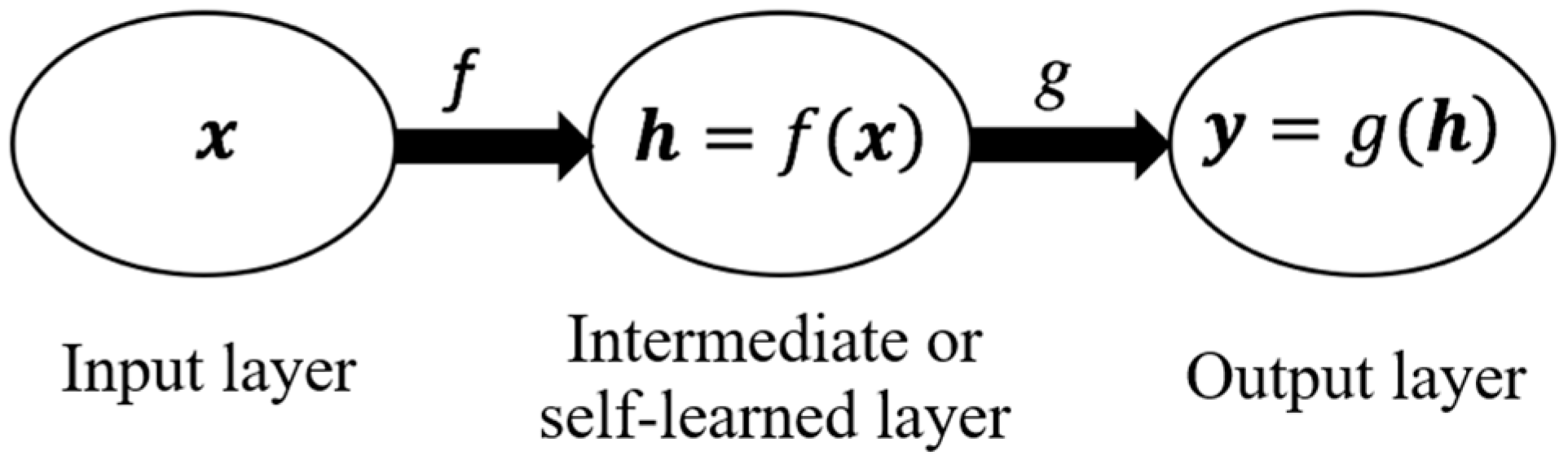
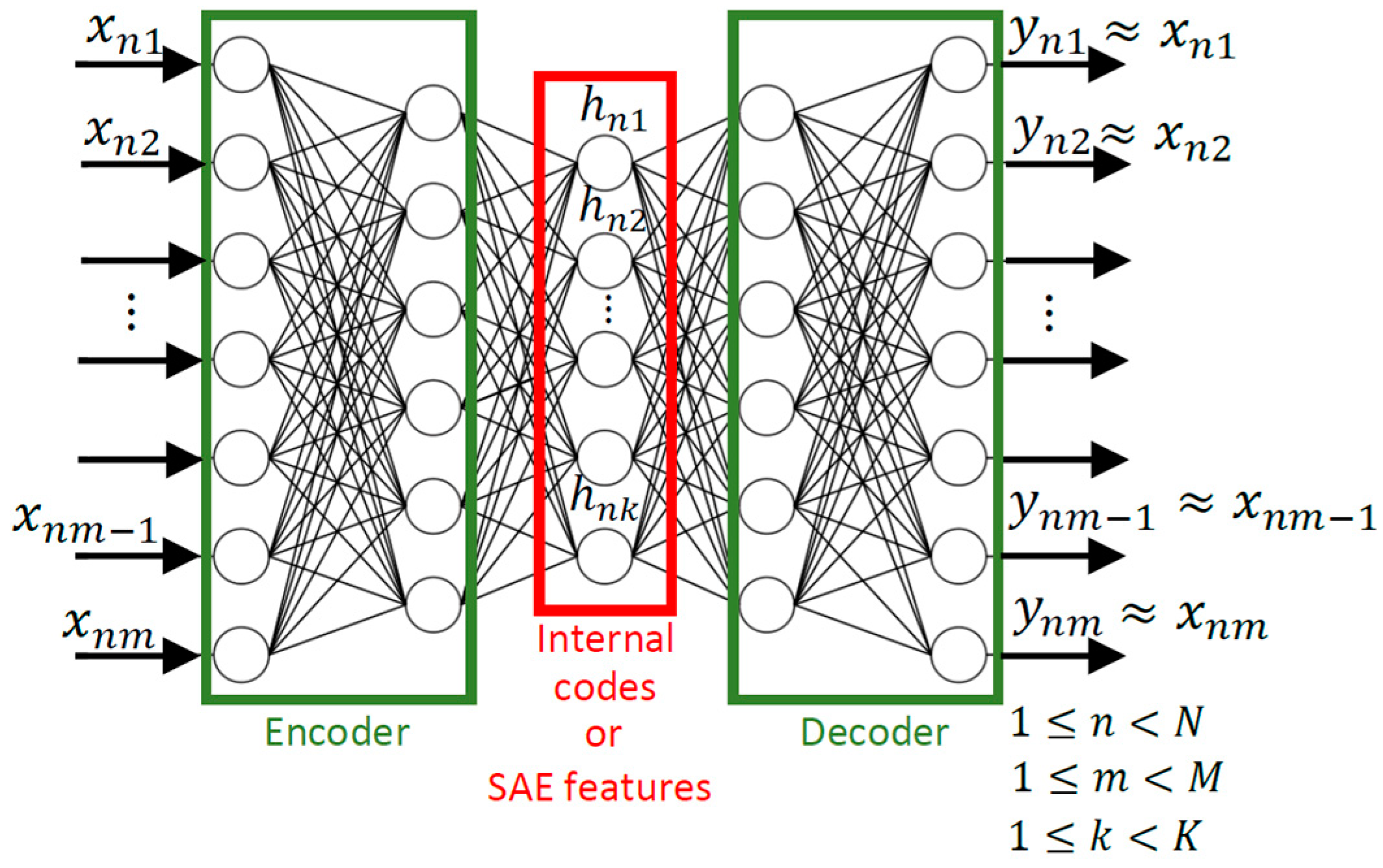
• Function f: represents the code function that operates over the input signal vector x (a single series of dynamic measurements, for instance).
• Vector h: stands for the result of a function f over a signal vector x. In other words, it is the feature vector.
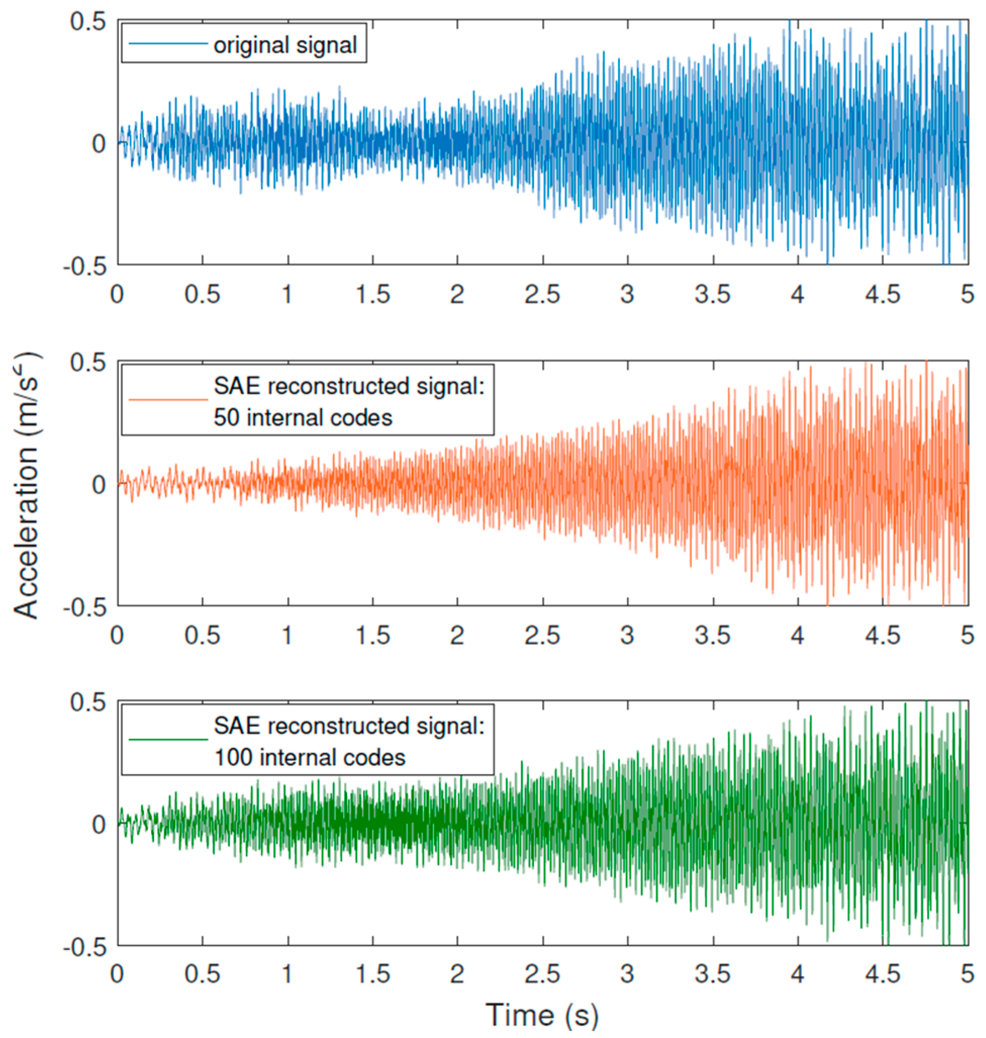
• Function g: represents the code function that operates over the feature vector h. This function reconstructs an approximation of the original input signal vector x.
• Vector y: stands for the result of a function g over the feature vector h. In other words, it is the reconstruction of the auto-encoder’s input.

The code function f applied to the input data x leads to the learned features $\mathit{h}=f\left(\mathit{x}\right)$. On the other hand, the decode function g applied to h leads to output $\mathit{y}=g\left(\mathit{h}\right)$. The principal idea is to write a cost function to calculate the AE parameters that produce $\mathit{y}\approx \mathit{x}$. At this point, it is important to observe that the learning process of an AE is unsupervised.

There are three possibilities for AE concerning the dimensionality of the h and x vector, K and M, respectively: For $K>M$, the complexity of $\mathit{h}$ is higher than the one of $\mathit{x}$ vector. This is not desirable if one wants to “learn” essential features of $\mathit{x}$. For $K=M$, this second hypothesis may be faced as a transformation of $\mathit{x}$, which also does not reduce the complexity of the problem. AEs placed on the third possibility ($K<M$) are called Undercomplete Auto Encoders, and they are often used for data mapping problems, like those addressed in the present work. The reduction of data’s dimension allows identifying significant parameters of $\mathit{x}$ that are appropriate for identifying structural damage ($\mathit{h}$ vector).

Instead of purely minimizing the cost function $Z\left(\mathit{x},g\left(f\left(\mathit{x}\right)\right)\right)$, which calculates the difference between $\mathit{x}$ and $\mathit{y}=g\left(f\left(\mathit{x}\right)\right)$, a sparse penalty ${\rm T}\left(f\left(\mathit{x}\right)\right)$ may be added in the function $Z$ during the training phase of the network. Function ${\rm T}\left(f\left(\mathit{x}\right)\right)$ is selected to increase the capacity of the AE to represent $\mathit{x}$ with a small number of $\mathit{h}$ components. In this case, the AE is called a Sparse Auto-Encoder (SAE). Goodfellow et al. (2016) [27] presented an excellent overview of AE and SAE, which is recommended for further inquiries.

To illustrate the above definitions, a typical SAE network is presented in Figure 2. It has an equal number of encoding and decoding layers (two in this figure) and a central layer from which the internal codes $\mathit{h}$ are derived. The symmetric configuration is mandatory for SAE networks. Both first and last layers (encoder and decoder, respectively) have $M$ processing units (neurons), $M$ being the sampled signals’ length. The central layer has $K$ neurons, corresponding to the $K$ internal components $\mathit{h}$ that are used to characterize each structural signal $\mathit{x}$ composed of $M$ data points. It is noteworthy that $K\ll M$, indicating the transformation of the input variables into new ones with a lower dimension. In order to achieve the objective of this work, the main SAE parameters—the number of encoding/decoding layers and the dimension of the vector $\mathit{h}$—are analyzed for two different structures, described further in the text. It is important to note that the feature vector $\mathit{h}$ is used to assess relevant information about the structure’s behavior. Then, such a vector is used as input to SVM for structural novelty detection.

SVM is a statistical machine learning method that has been widely used to solve several pattern recognition problems. The fundamental idea of SVM is to construct an optimal separating hyperplane by maximizing the margin and minimizing the misclassification between two classes of data in a space [39]. The SVM performs the classifications by defining some training data points positioned in the margins (support vectors), where the distance between them is maximized through an optimization function that minimizes the Euclidean norm of the hyperplane’s directional vector. When dealing with nonlinear problems, the input variables are mapped in a higher-dimensional feature space by using a kernel function. The SVM theory can be extended to multi-class classification problems through strategies based on a combination of binary classifiers, e.g., one-against-one and one-against-all [40]. For more detailed information about SVM, see Vapnik (2013) [39] and Bishop (2006) [40].

3. The Adopted SHM Strategy

This section describes the SHM strategy used to evaluate SAE’s performance, summarized in two main steps:

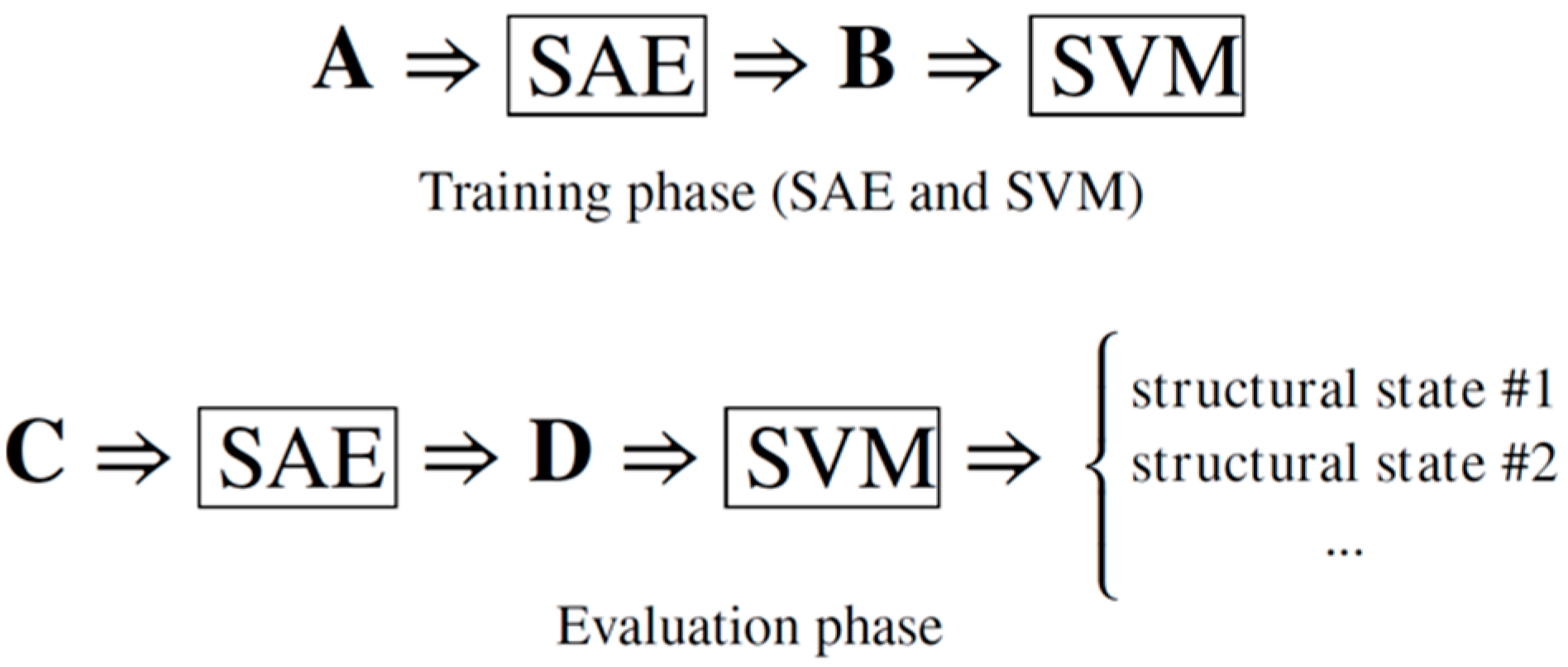
• Training phase

  (a)

  Data organization. An input training matrix A with ($P\times M$) elements is created, P being the number of dynamic tests randomly selected for the training phase, where M is the sampled signals’ length. Thus, matrix A is formed by arranging each selected vector x in a row of the input matrix. In other words, matrix A gathers the dynamic measurements.

  (b)

  Data characterization using SAE. This task is conducted in an unsupervised way via SAE, using matrix A. The penalization function $Z\left(\mathit{x},g\left(f\left(\mathit{x}\right)\right)\right)$ is minimized and, for each vector x, a corresponding vector h is obtained. An SAE output matrix B with its ($P\times K$) elements is organized with the output vectors h. It can be said that matrix B “collects” the feature vectors. The minimization is performed through a feedforward backpropagation algorithm employing the Scaled Conjugate Gradient (SCG) optimization method [41]. Furthermore, hyperparameters, such as the sparsity proportion $\rho$, sparsity regularization $\beta$ and weight regularization $\lambda$, were selected empirically. These parameters are related to the sparse penalty function defined in Section 2 and assist in the determination of the best solution by the SAE [42].

  (c)

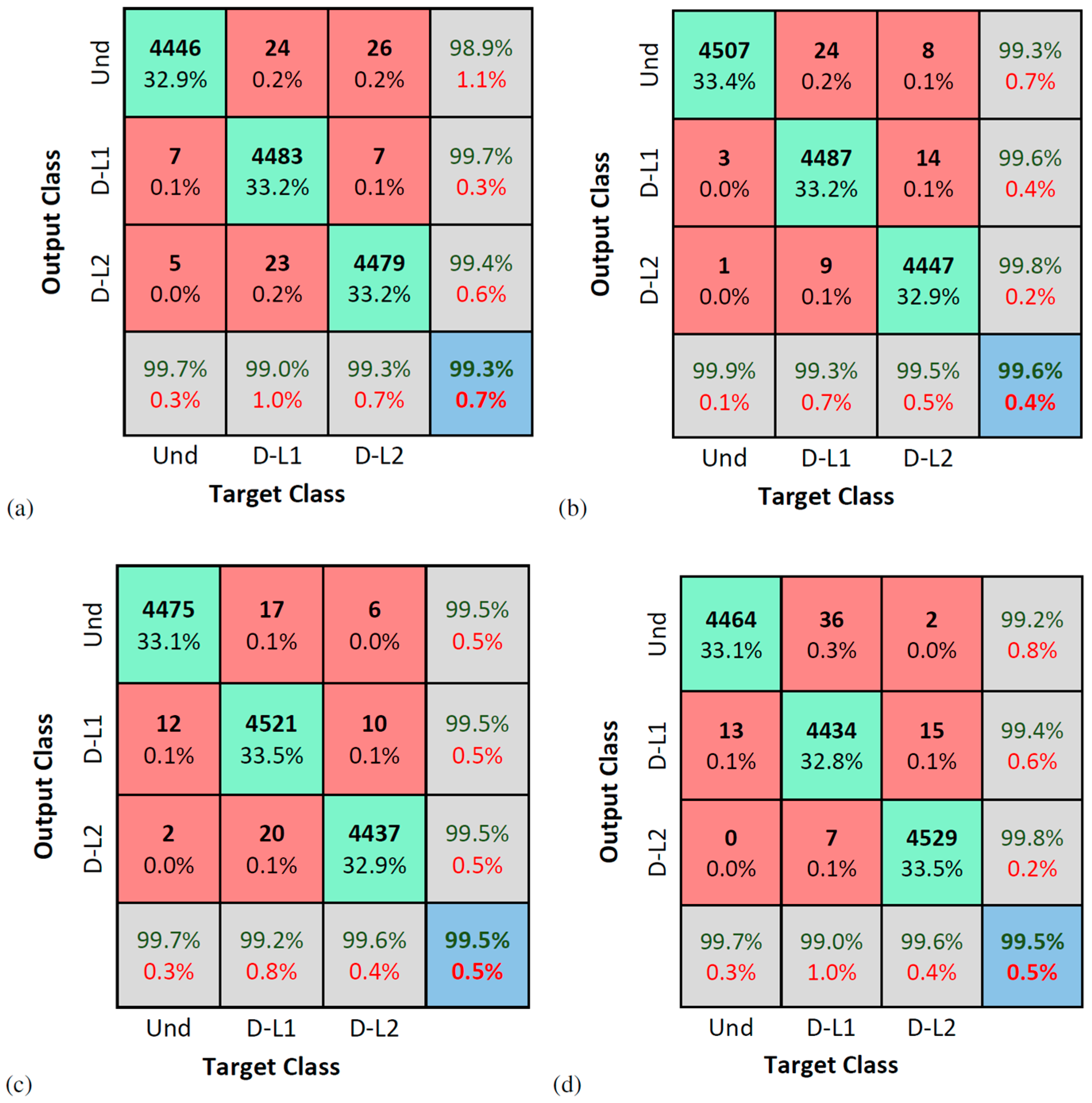
  Data classification using SVM. Although the signal characterization is unsupervised, the data classification model’s training process is supervised, since the pattern recognition herein is carried out using classical SVM. Hence, matrix B and its respective targets (referring to the structural conditions) are utilized for training the SVM. In this case, the SVM model is constructed using the Radial Basis Function (RBF) kernel and considers the one-against-one strategy to solve the multi-class problems. The parameters $\sigma$ and $C$ (regularization terms from the RBF kernel and maximization formulation, respectively) were estimated through an exhaustive search procedure known as Grid Search [43] applying the 10-fold cross-validation [44].

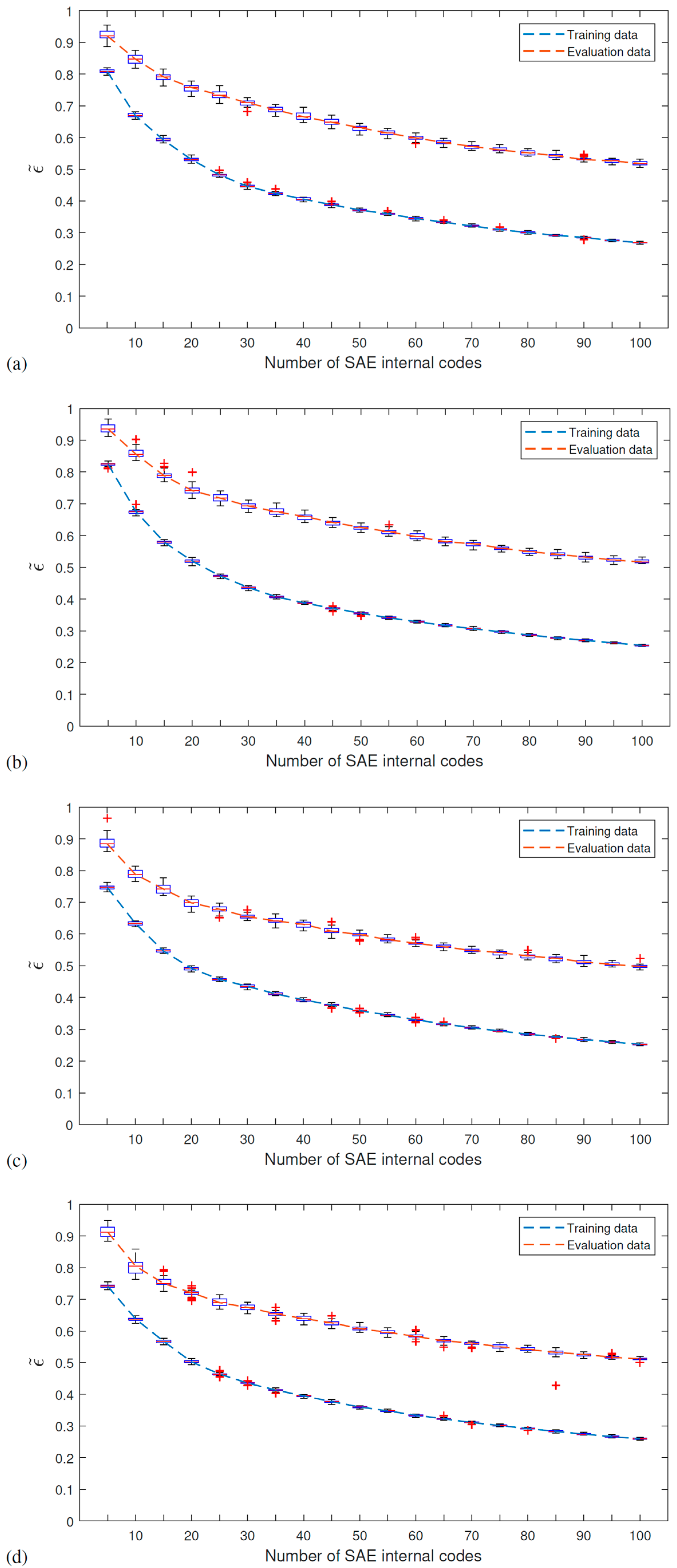
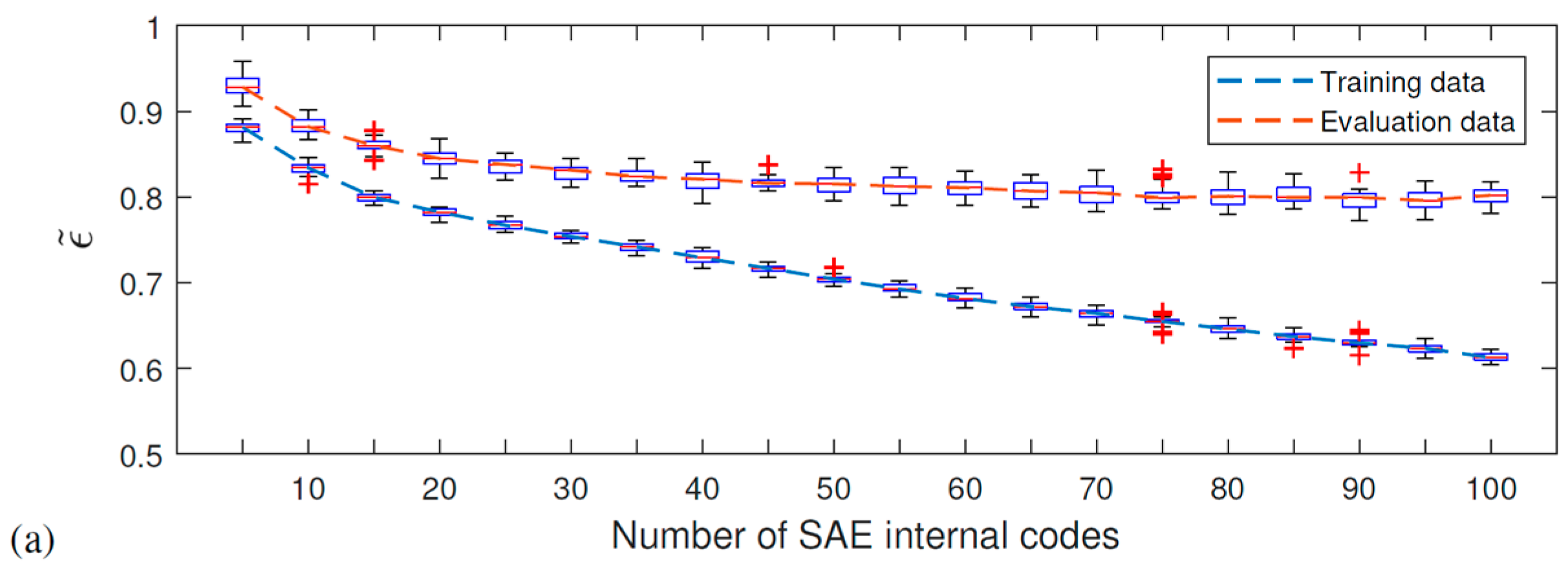
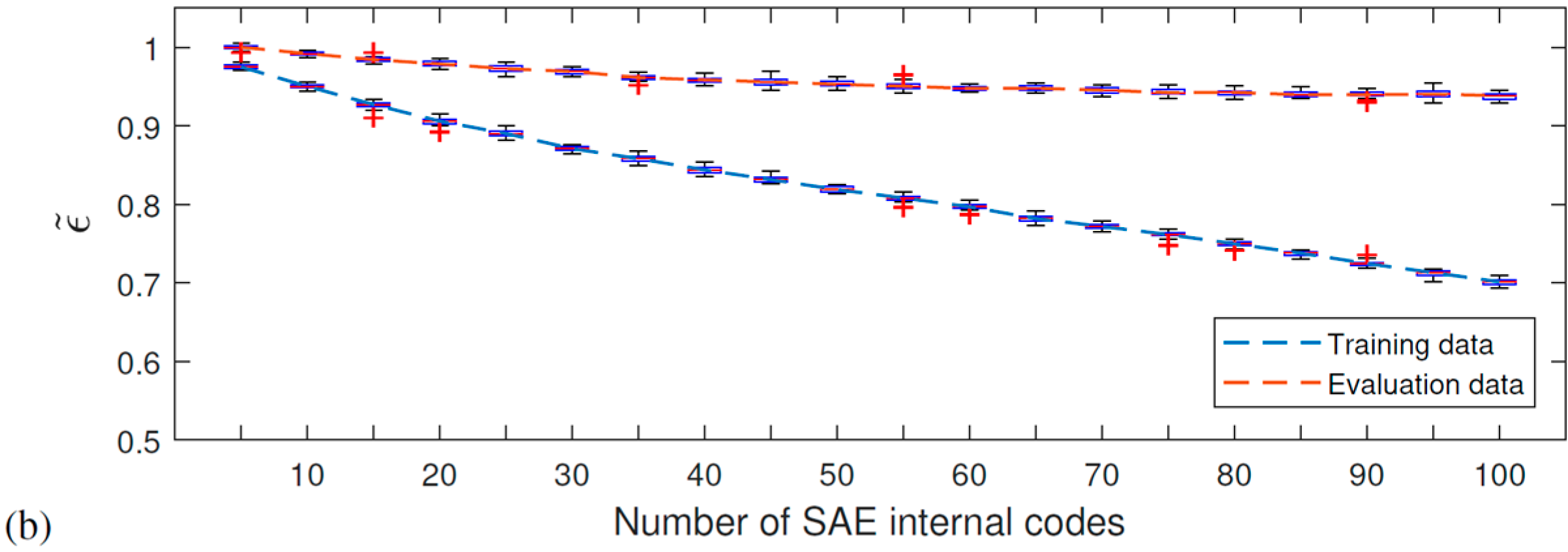
• Evaluation phase. Assuming that the SVM models are well-trained and achieve acceptable classification rates, the performance of the proposed SHM strategy is directly linked to the SAE’s capability to extract features from the dynamic signals adequately. The current step is developed by evaluating the set of dynamic measurements that were not used in the previous phase, gathered in matrices $\mathit{C}$ and $\mathit{D}$. Matrix $\mathit{C}$, containing $Q$ vectors $\mathit{x}$ (being $N=P+Q$, where $N$ is the number of available dynamic signals), is presented to the trained SAE network, resulting in a matrix $\mathit{D}$ with the respective vectors $\mathit{h}$. Finally, matrix $\mathit{D}$ is presented to the trained SVM, whose output is the structural condition.

Figure 3 schematically illustrates the two main steps of the SHM strategy.

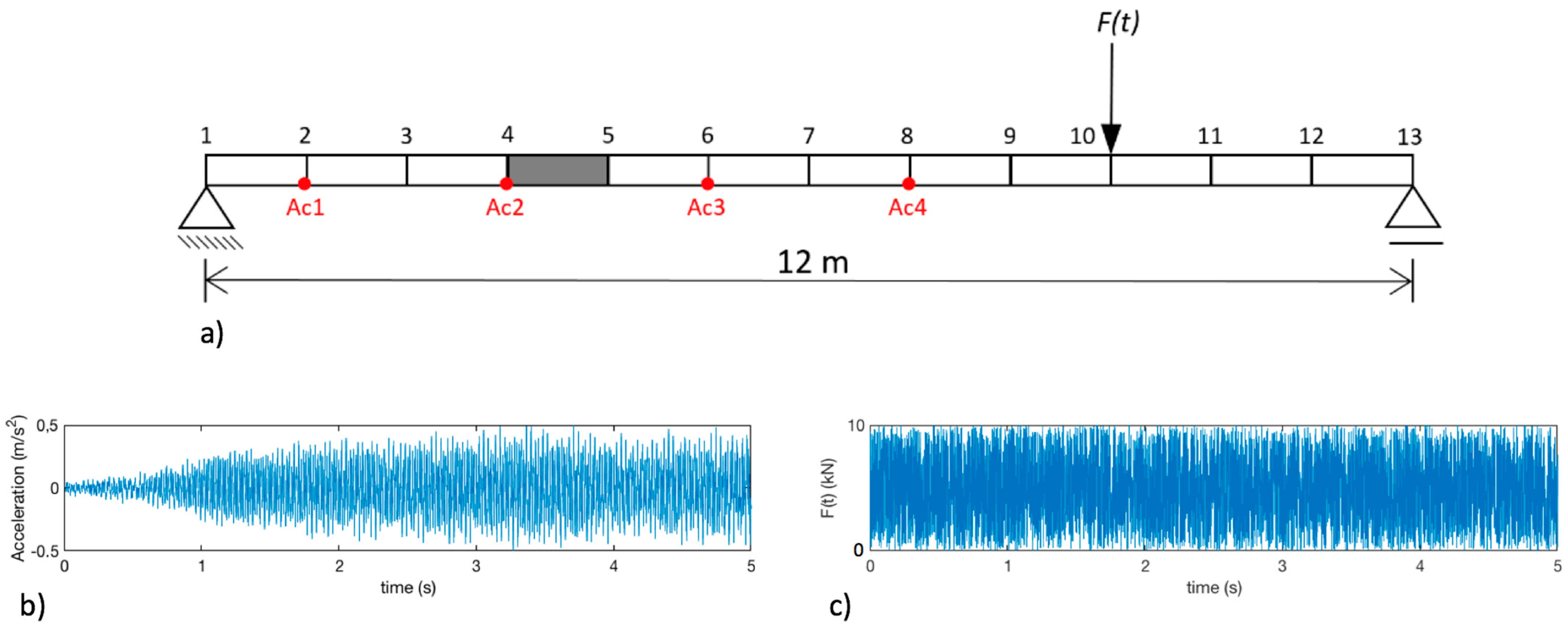
4. Numerical Application: Simply Supported Beam

In order to initially evaluate the SAE’s efficiency to characterize vibration data, numerical simulations are performed using a simply supported beam model (see Figure 4a). The beam is modeled with twelve Euler-Bernoulli elements (two degrees of freedom per node - one translation and one rotation) with the following properties: total length = $12 \mathrm{m}$; Young’s modulus = $210 \mathrm{G}$Pa; cross-section area = $0.04 {\mathrm{m}}^2$; specific mass = $7850 {\mathrm{kg} \mathrm{m}}^{-3}$ and moment of inertia = $5.33\times {10}^{-4}{ \mathrm{m}}^4$. The numerical integration is performed by using Newmark’s method with a time step of 0.001 s. The excitation force $F\left(t\right)$ is a typical random vector with 10 kN of maximum magnitude, which is randomly set for every dynamic simulation carried out and is applied at node 10. $F\left(t\right)$ (kN) is simulated as shown in Equation (1):

$$F\left(t\right)=10\times V~D\left(0,1\right)$$

(1)

where $V~D\left(0,1\right)$ is a vector with random values extracted from a uniform distribution from 0 to 1. Figure 4b,c present a typical response of the system for a random excitation force F(t), respectively.

Three structural damage scenarios were simulated: healthy structure, damage level #1, and damage level #2. The first and second damage levels were defined by reducing in 10% and 20%, respectively, the Young’s modulus of element #4 from the undamaged structural model (depicted in Figure 4 by the gray element). The vertical dynamic responses of points 2 (Ac1), 4(Ac2), 6(Ac3) and 8(Ac4) were recorded in terms of accelerations and were used to evaluate the SAE-based damage detection methodology. Each vibration signal lasts 5 s and has 5001 discrete time samples (sampling frequency of 1000 Hz). The structure’s natural frequencies in all assumed conditions are given in

Table 1. Variation of the numerical beam eigenfrequencies.

Structural Scenario	1st Natural Frequency	2nd Natural Frequency	3rd Natural Frequency	4th Natural Frequency
Healthy	6.51 Hz	26.06 Hz	58.65 Hz	104.32 Hz
Damage level 1	6.21 Hz	25.04 Hz	56.53 Hz	100.30 Hz
Damage level 2	5.88 Hz	23.92 Hz	54.22 Hz	96.03 Hz

, merely for information purposes.

Three hundred different numerical simulations for each structural stage were generated by varying the excitation, totaling 900-time histories per measurement point ($N$ = 900 available dynamic signals). Since the excitation is random, the structure’s dynamic responses are also random. The proposed SHM approach is evaluated by investigating the signals from one point at a time. Thus, the entire dataset is organized in four input matrices [900 $\times$ 5001] (900 dynamic time histories composed of 5001 time samples), corresponding to the responses measured in positions Ac1, Ac2, Ac3 and Ac4. Since the SVM classifies the data category, it is also necessary to indicate the damage class of the signals. For this reason, a target matrix [900 $\times$ 3] is assembled, specifying in its rows the respective signal category through the binary code: (1 0 0)—healthy beam; (0 1 0)—damage level #1; and (0 0 1)—damage level #2. It is worth mentioning that the target matrix is only used in the SVM training phase. During the evaluation phase, these labels have no direct participation in the classification. They are only applied to compare the results obtained by the SVM with the actual structure degradation level.

Before being processed by SAE, the signal matrices are normalized within the range [−1;1]. The goal of normalization is to change the values of numeric columns in the dataset to use a common scale, without distorting differences in the ranges of values or losing information [45]. Afterwards, the input matrices—and consequently, the target matrices—were randomly subdivided into other two matrices, allocating 50% of the signals for the training phase—matrix $\mathit{A}$ [450 $\times$ 5001]—and the remaining 50% of data for the evaluation phase—matrix $\mathit{C}$ [450 $\times$ 5001]. In order to guarantee that all structural scenarios are equally represented in the SAE and SVM models, the training and evaluation matrices should have approximately the same number of samples from each damage level (balanced dataset). For further information about this subject, see Japkowicz and Stephen (2002) [46].

Subsequently, matrix $\mathit{A}$ is used to construct the SAE model to “learn” representative features directly from acceleration responses expressed in the time domain. For all analyses, the SAE models were implemented considering encoder and decoder layers. Different numbers of neurons (internal codes $\mathit{h}$) were evaluated. In the last part of the training process, the attributes extracted by SAE are passed as input parameters (matrix $\mathit{B}$) to an SVM that creates a model aimed at identifying the corresponding damage classes.

Finally, the remaining data—matrix $\mathit{C}$ and its derivative matrix $\mathit{D}$, not used in the training phase—are presented to the machine learning models to test their real effectiveness, indicating the different structural conditions. The proposed SHM approach was developed using toolboxes and built-in functions available in Matlab.

Table 2. SAE and SVM parameters of the proposed strategy for the numerical beam example.

SAE Parameters
Sparsity proportion ($\rho$)	0.050
Sparsity regularization ($\beta$)	4.000
Weight regularization ($\lambda$)	0.001
Encoder/decoder activation functions	Logarithmic sigmoid/linear
Optimization method	Scaled Conjugate Gradient
Gradient maximum value	1.00E-6
Max. of training epochs	1000
Training error metric	Mean-squared error
SVM Parameters
Kernel function	RBF
Multiclass coding scheme	One-vs-one
$\sigma$—for 50 SAE internal codes	1.0000
$\sigma$—for 100 SAE internal codes	1.5000
$\mathit{C}$—for 50 SAE internal codes	0.3162
$\mathit{C}$—for 100 SAE internal codes	0.3162

shows the parameters of the achieved SAE and SVM models.

Results

Since the damage identification of the proposed strategy is based on the features extracted by the SAE, the first stage of the analysis examines how many SAE internal codes are necessary for a good representation of the dynamic structural responses. As previously mentioned, the SAE training is performed by reconstructing its input data. Therefore, it is reasonable that the difference between the original and the reconstructed signals may indicate whether the extracted characteristics contain relevant information about the structural response or not. In the present paper, this difference is denoted as reconstruction error $ϵ$, and is individually calculated by Equation (2):

$${ϵ}_j=\frac{{{\displaystyle \sum }}_{i=1}^M\left|x_{ji}-{\widehat{x}}_{ji}\right|}{{{\displaystyle \sum }}_{i=1}^M\left|x_{ji}\right|},$$

(2)

where $M$ is the total length of the sampled signal, and $x_{ji}$ and ${\widehat{x}}_{ji}$ are the ith element of the jth original signal vector $\mathit{x}$ and the jth SAE reconstructed signal vector $\widehat{\mathit{x}}$, respectively ($j=1, \dots , J$, $J$ being the length of the corresponding analyzed dataset). For the complete set of dynamic signals, the reconstruction error is the mean of all errors ${ϵ}_j$, as given in Equation (3):

$${\widetilde{ϵ}}_j=\frac{1}{J}{\displaystyle \sum }_{j=1}^J{ϵ}_j.$$

(3)

Figure 5 shows a box plot evolution of the error $\widetilde{ϵ}$ as the amount of SAE features increases for all selected points of the numerical beam example. Each box was created by considering 30 different SAE models that reduce the problem’s dimensionality from 5001-time samples to the indicated number of internal codes (vector $\mathit{h}$). The thirty different SAE models are auto-encoder models developed with the same parameters but varying in the random seed. The boxes associated with the blue dashed line indicate the reconstruction performance of the 30 models for data used during the training phase. The boxes related to the red dashed line, on the other hand, correspond to the reconstruction errors of the same models when applying unseen data (evaluation phase).

In Figure 5, it is possible to observe that the plotted curves are quite similar for all simulated accelerometer channels. In all cases, the median of training and evaluation errors tends to have a linear behavior as the number of internal codes increases. For 100 SAE characteristics (internal codes), $\widetilde{ϵ}$ achieves values around 0.25 and 0.50 for training and evaluation data, respectively. Moreover, although not represented in the graphs the same linear behavior was verified for SAE models, with more than 100 internal codes (from 100 to 500). Obviously, the greater the number of SAE features, the better the signal reconstruction and the smaller the errors $\widetilde{ϵ}$. However, the focus of this work is not to exactly reconstruct the signal, but to extract key elements capable of characterizing the differences between “normal” and “abnormal” structural responses. Figure 6 displays an example of the SAE reconstructed response when using 50 and 100 internal codes in comparison with their respective original signals. Both plots reveal that just a reduced number of SAE features are enough to fairly represent the original simulated accelerations. For this reason, the authors opted to classify the data with 50 and 100 SAE characteristics (the start and the end of the linear behavior region exhibited in the graph). It can also be noted that the reconstruction errors of the training data are smaller than those obtained for the evaluation data, regardless of the number of SAE characteristics. This is an expected result, given that the first group of data was used to create the SAE models, and the second one has never been presented to them.

The performance of the proposed approach for 30 different SAE/SVM models developed with 50 and 100 internal codes, respectively, is presented in

Table 3. Simply supported numerical beam: correct classification rates in percentage.

	Mean		Max.		Min.		Std. Deviation
SAE Internal Codes	50	100	50	100	50	100	50	100
Ac1	99.32	99.96	100.00	100.00	98.22	99.78	0.46	0.08
Ac2	99.56	99.99	100.00	100.00	98.22	99.78	0.43	0.04
Ac3	99.50	99.93	100.00	100.00	98.67	99.56	0.35	0.12
Ac4	99.50	99.94	100.00	100.00	98.89	99.56	0.38	0.13

. The classification rate is the mean value of correct identifications achieved in each model (average of the 30 models), only considering the evaluation data. Figure 7 and Figure 8 show the confusion matrices related to the classification rates obtained in Table 3. These matrices point out the classification frequencies of the evaluation examples along with the three structural conditions. The diagonal elements in green are the amount and percentage of correct classifications, whereas the red elements refer to the amount and percentage of misclassified data. The rightmost column of the matrix exposes the precision metric (true positives/(true positives + false positives), and the row at the bottom exposes the recall metric (true positives/(true positives + false negatives). The element in the bottom right of the plot represents the overall accuracy. The “Output Class” corresponds to the predicted damage level and the “Target Class” to the level which the signal really belongs. They were constructed with all evaluating subsets, resulting in 13,500 different analyzed examples (450 evaluating examples $\times$ 30 models).

The classification averages are greater than 98% with standard deviation values below 0.5% for all measurement points, indicating the ability of the SAE to interpret and to extract features directly from structural acceleration time histories. Despite the good performance obtained for both quantities of SAE characteristics tested, the accuracy is slightly higher for models with 100 internal codes. For this configuration, practically 100% of the data were correctly classified. The confusion matrices confirm these results.

Figure 8. Simply supported numerical beam: Confusion matrices—100 SAE internal codes. (a) Measurement point Ac1. (b) Measurement point Ac2. (c) Measurement point Ac3. (d) Measurement point Ac4.

Figure 8. Simply supported numerical beam: Confusion matrices—100 SAE internal codes. (a) Measurement point Ac1. (b) Measurement point Ac2. (c) Measurement point Ac3. (d) Measurement point Ac4.

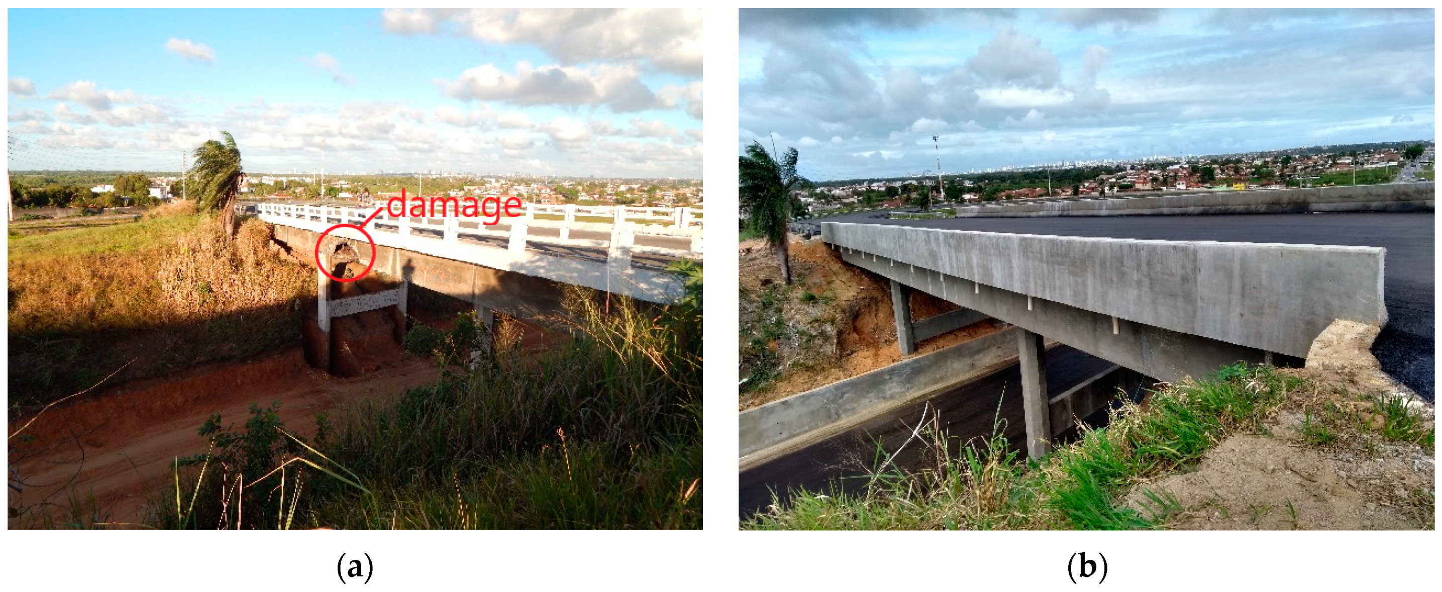
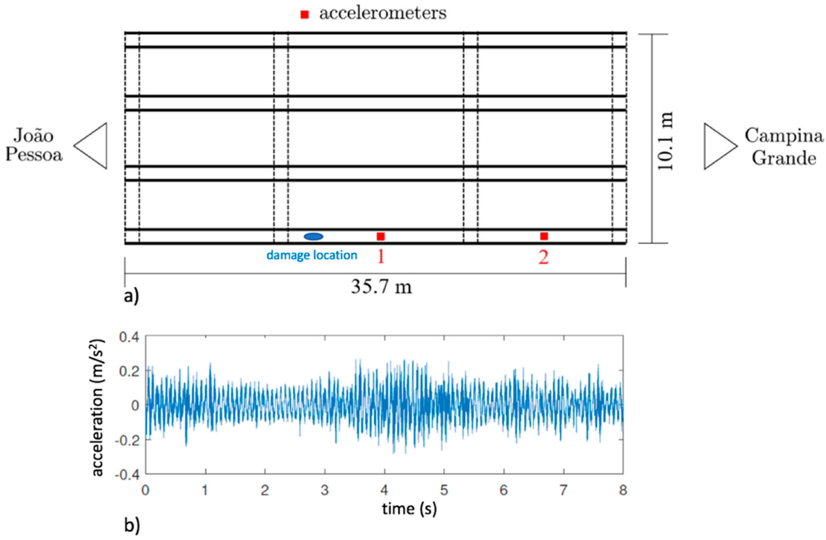
5. Experimental Application: Várzea Nova Viaduct

The second application is the Várzea Nova viaduct situated in Paraíba at the intersection of highways BR-101 and BR-230, between the towns of João Pessoa and Campina Grande, in Brazil. The viaduct is 35.7 m long, and due to a traffic accident, one of the four main girders was damaged. To fix it and also to comply with Brazil’s current regulation codes, a series of procedures were implemented, including strengthening of pillars, beams, deck, and foundation. Figure 9 shows a perspective view of the viaduct.

Dynamic tests were conducted before and after structural reinforcement, leading to sets of experimental time histories (accelerations) obtained under traffic loading. A National Instruments NI9215 acquisition system attached to a computer was used to process the vibration signals that were collected by two piezoelectric accelerometers ENDEVCO model 752A13, positioned on the deck above the right border girder at its midspan and at its one-sixth length, as shown in Figure 10. Four dynamic tests were performed for each structural condition, resulting in 8 tests to be analyzed per accelerometer channel. Each structural response has 512 s sampled at 512 Hz. The variation of the first natural frequency—before and after the strengthening—is shown for information purposes in

Table 4. Variation of the first natural frequency of the Várzea Nova viaduct.

Structural Scenario	1st Natural Frequency
Before strengthening	13.37 Hz
After strengthening	13.76 Hz

. As expected, higher values can be observed on the fundamental frequency after the strengthening, since this procedure increased the structure’s stiffness without significantly changing it mass.

To allow a parallel with the beam’s signals with respect to the number of sampled points and the number of cycles analyzed per second, the viaduct vibration measurements were divided into more signals before processing the structural responses with SAE. Hence, each accelerometer provided 512 8-s long signals arranged in input matrices (512 $\times$ 4096), corresponding to 256 dynamic time histories collected before the strengthening procedure and the other 256 collected after. Given the SVM supervised learning, a 512-position target vector was generated specifying the data category through the binary code: 0—before the strengthening, and 1—after the strengthening. In this case, the signal matrices are scaled into (−10;10) to prevent the quadratic error magnitude from causing significant numerical problems capable of hindering the convergence of the optimization method, as verified in some initial tests.

For the present application, it was opted to assign approximately 70% of signals to the training phase and 30% to the evaluation phase, as a result of the lower number of structural responses available when compared to the numerical beam. One of the 512 signals of the accelerometer 2 was discarded due to acquisition problems verified during the data organization step. Therefore, the input matrices, as well as the target vectors, were subdivided into matrix $\mathit{A}$ (362 $\times$ 4096) for both accelerometer channels and into matrix $\mathit{C}$ (150 $\times$ 4096) for the accelerometer 1, and into matrix $\mathit{C}$ (149 $\times$ 4096) for the accelerometer 2. The architecture and parameters of the achieved SAE and SVM models for the Várzea Nova viaduct are in

Table 5. SAE and SVM parameters of the proposed strategy for the Várzea Nova viaduct.

SAE Parameters
Sparsity proportion ($\rho$)	0.050
Sparsity regularization ($\beta$)	4.000
Weight regularization ($\lambda$)	0.001
Encoder/decoder activation functions	Logarithmic sigmoid/linear
Optimization method	Scaled Conjugate Gradient
Gradient maximum value	1.0 × 10−6
Max. of training epochs	1000
Training error metric	Mean-squared error
SVM Parameters
Kernel function	RBF
Multiclass coding scheme	One-vs-one
$\sigma$—for 50 SAE internal codes	0.3162
$\sigma$—for 100 SAE internal codes	0.3162
$\mathit{C}$—for 50 SAE internal codes	0.3162
$\mathit{C}$—for 100 SAE internal codes	0.0316

.

Results

The $\widetilde{ϵ}$ convergence curves (see Equations (2) and (3)) of the Várzea Nova viaduct are exhibited in Figure 11. Several numbers of internal codes were tested considering 30 different SAE models, in which the dimensionality of the problem reduces from 4096 time samples to the specified quantity of characteristics $\mathit{h}$. The error evolution behavior for the viaduct signals is similar to the ones observed in the first example analyzed in this paper. Even so, the reconstruction errors of the present structure stabilize at higher values than in the numerical beam. While the error $\widetilde{ϵ}$ of the beam evaluation data reaches values around 0.5 for 100 internal codes, the error for the viaduct evaluation data stabilizes at values above 0.8. This is an expected result, since experimental data are normally more susceptible to noise. Besides, these viaduct plots also confirm the lower reconstruction errors for the training data. As with the beam analysis, a visual representation example of the SAE model reconstruction performance for 50 and 100 internal codes is shown in Figure 12. It is possible to observe that the reconstructed signal with 50 internal codes alludes to the original structural response. However, the improvement in the reconstruction of the signal obtained with 100 SAE characteristics is clearly visible.

Table 6. Várzea Nova viaduct: correct classification rates in percentage.

	Mean		Max.		Min.		Std. Deviation
SAE Internal Codes	50	100	50	100	50	100	50	100
Accelerometer 1	99.80	100.00	100.00	100.00	98.67	100.00	0.43	0.00
Accelerometer 2	92.10	96.78	97.99	99.33	87.25	91.95	2.62	1.87

, as well as the confusion matrices of Figure 13 and Figure 14, present the classification rates of the proposed damage detection methodology for 30 different SAE/SVM models developed with 50 and 100 internal codes respectively. They were assembled considering all evaluation subsets; thus, 4500 different examples were analyzed for accelerometer 1 (150 evaluating examples $\times$ 30 models) and 4470 for accelerometer 2 (149 evaluating examples $\times$ 30 models).

According to the results, the SAE was efficient to characterize the viaduct vibration signals with both 50 or 100 internal codes. The classification rates were all above 85% with very low deviations (maximum value of 2.62%), highlighting the excellent performance achieved by the models with signals of accelerometer 1 reconstituted from 100 SAE features (total accuracy of 100% and zero standard deviation). In fact, the overall accuracy percentages also reflect the better signal reconstruction for 100 SAE internal codes verified in Figure 12. Moreover, it is possible to see that the worst classification rates are associated with signals from accelerometer 2. This outcome may be attributed to the position of accelerometer 2, which is less affected by the first natural frequency than of accelerometer 1 (placed exactly at the midspan).

An interesting aspect could be noticed by interpreting the confusion matrices is the SAE/SVM capacity to correctly identify the “after strengthening” data. In all cases, no signal belonging to the class “after strengthening” was misclassified as being “before strengthening” (the recall values are equal 100%). Regarding the few “before strengthening” signals incorrectly recognized, even in the less favorable scenario—when 353 “before strengthening” examples from accelerometer 2, reconstructed with 50 internal codes, were classified as “after strengthening”—the results can still be considered as acceptable.

6. Conclusions

This paper investigated the use of a Sparse Auto-Encoder to characterize vibration signals aiming to detect structural anomalies. Features extracted by SAE directly from time-domain accelerations were used as input variables to train a classification model based on the traditional Support Vector Machine. Firstly, the proposed methodology was checked using structural responses from a numerical model of a simply supported beam under different damage levels. Then, in order to verify the SAE/SVM effectiveness in a real-case structure, experimental data from Várzea Nova viaduct in João Pessoa (Brazil) were analyzed. Dynamic tests under local traffic were performed on the viaduct before and after a reinforcement procedure.

For both structures, the proposed approach was able to identify practically all dynamic responses correctly:

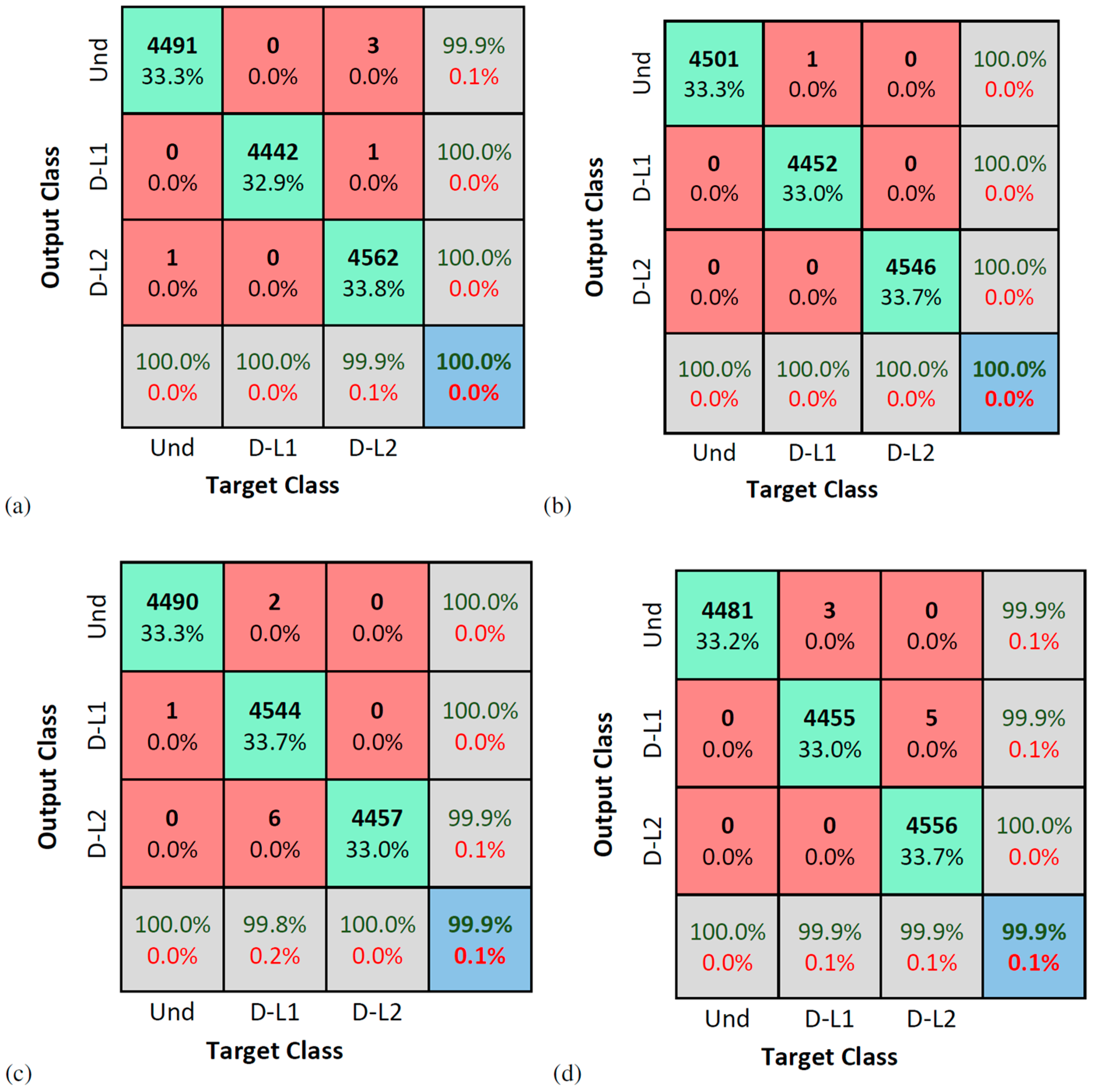
• For the numerical model, the two damage scenarios were almost perfectly detected, indicating that the proposed method is sensitive to the damage level, corroborating its potential for multiple damage and damage quantification problems.
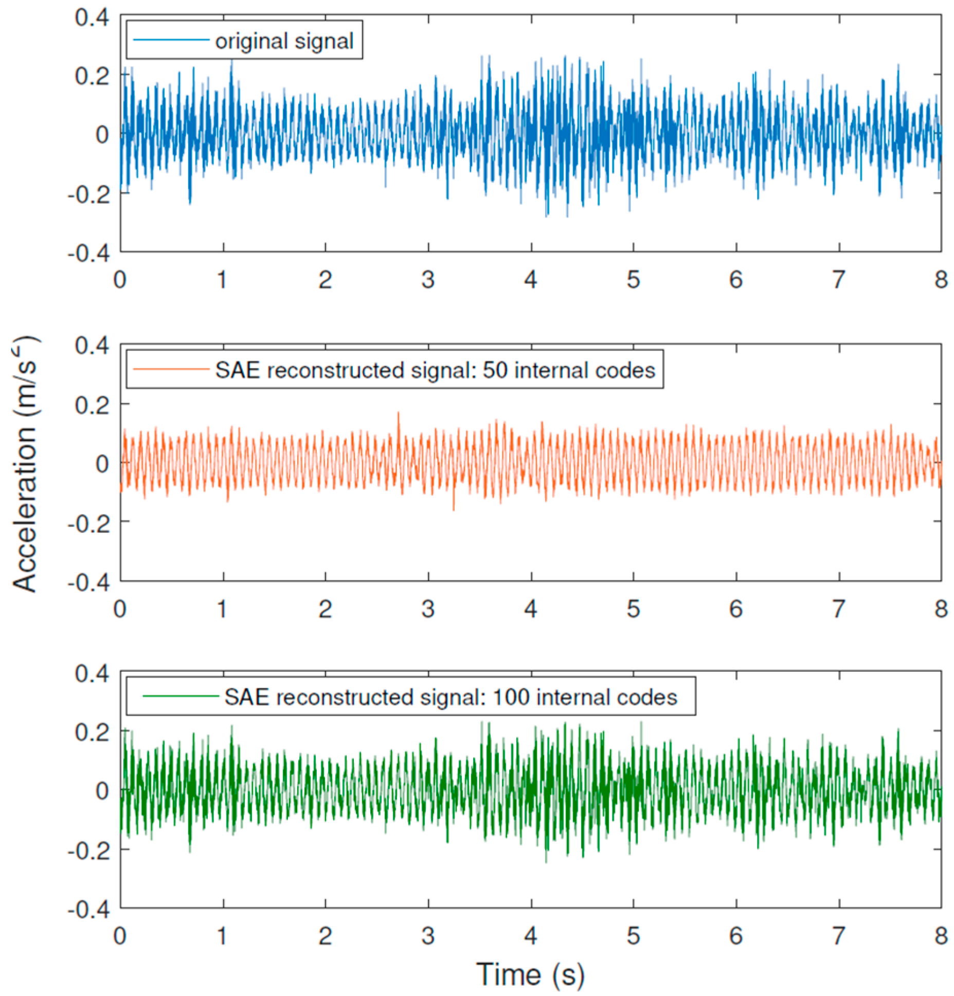
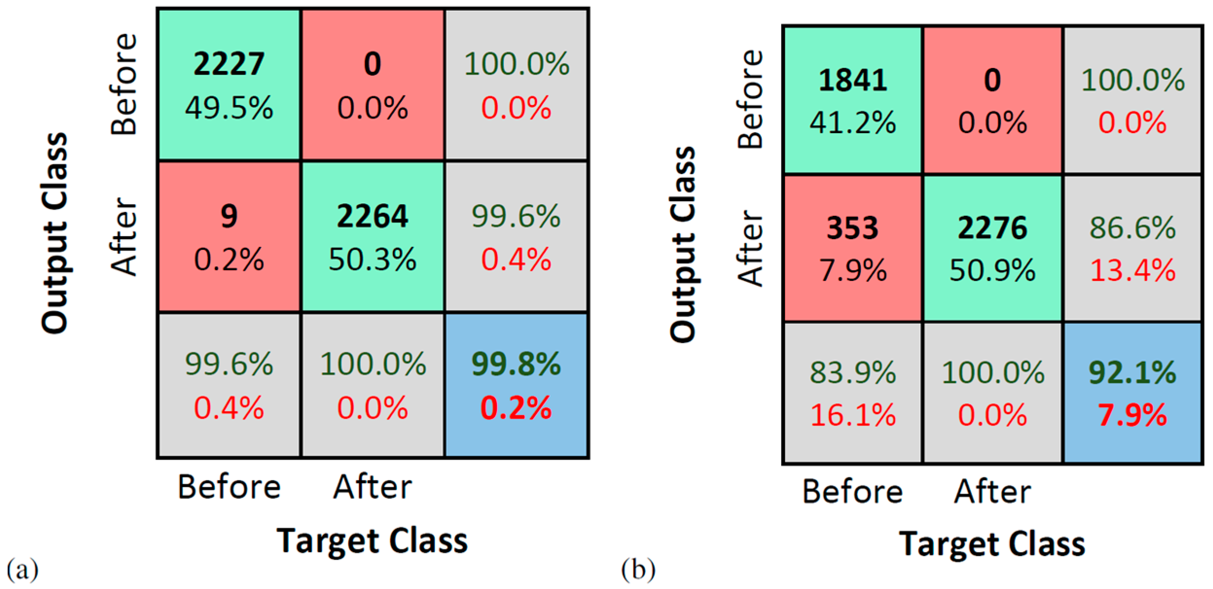
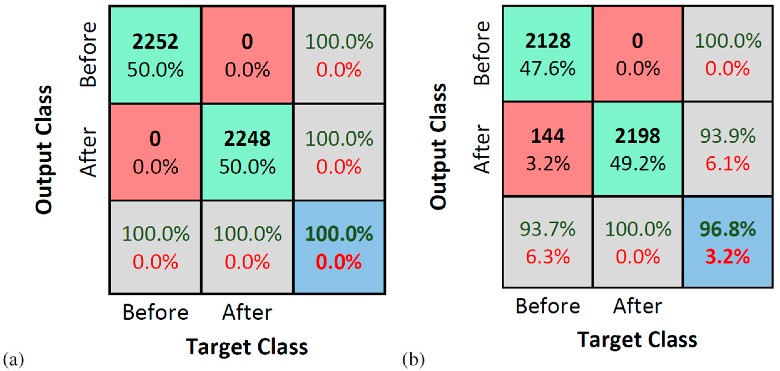
• For the Várzea Nova viaduct tests, the performance was slightly inferior due to the influence of external factors, such as noise, traffic, temperature, among others. Furthermore, even though better classification rates were obtained for signals reconstructed with 100 SAE characteristics, the results for dynamic data reconstituted with 50 features were more than reasonable. It is also important to highlight that the SAE features extracted have only 1% or 2% of the total signal’s length, for 50 or 100 internal codes, respectively. In addition, the performance of the proposed technique for the accelerometer closest to the damage was superior, which may indicate that the proposed methodology can be better explored in damage location problems.

Finally, the above considerations encourage the development of computational models using SAE for structural integrity assessment.

References

- Azim, M.R.; Gül, M. Data-driven damage identification technique for steel truss railroad bridges utilizing principal component analysis of strain response. Struct. Infrastruct. Eng. 2021, 17, 1019–1035. [Google Scholar] [CrossRef]
- Nunes, L.A.; Amaral, R.P.F.; Barbosa, F.S.; Cury, A.C. A hybrid learning strategy for structural damage detection. Struct. Health Monit. 2021, 20, 2143–2160. [Google Scholar] [CrossRef]
- Wah, W.S.L.; Chen, Y.-T.; Owen, J.S. A regression-based damage detection method for structures subjected to changing environmental and operational conditions. Eng. Struct. 2021, 228, 111462. [Google Scholar]
- Doebling, S.W.; Farrar, C.R.; Prime, M. A Summary Review of Vibration-Based Damage Identification Methods. Shock. Vib. Dig. 1998, 30, 91–105. [Google Scholar] [CrossRef] [Green Version]
- Avci, O.; Abdeljaber, O.; Kiranyaz, S.; Hussein, M.; Gabbouj, M.; Inman, D.J. A review of vibration-based damage detection in civil structures: From traditional methods to Machine Learning and Deep Learning applications. Mech. Syst. Signal Process. 2020, 147, 107077. [Google Scholar] [CrossRef]
- Yang, C.; Oyadiji, S.O. Damage detection using modal frequency curve and squared residual wavelet coefficients-based damage indicator. Mech. Syst. Signal Process. 2017, 83, 385–405. [Google Scholar] [CrossRef]
- Liu, G.; Zhai, Y.; Leng, D.; Tian, X.; Mu, W. Research on structural damage detection of offshore platforms based on grouping modal strain energy. Ocean Eng. 2017, 140, 43–49. [Google Scholar] [CrossRef]
- Marrongelli, G.; Gentile, C.; Saisi, A. Anomaly Detection Based on Automated OMA and Mode Shape Changes: Application on a Historic Arch Bridge. In Proceedings of the ARCH 2019, 9th International Conference on Arch Bridges, Porto, Portugal, 2–4 October 2019; pp. 447–455. [Google Scholar]
- Gillich, G.-R.; Furdui, H.; Wahab, M.A.; Korka, Z.-I. A robust damage detection method based on multi-modal analysis in variable temperature conditions. Mech. Syst. Signal Process. 2019, 115, 361–379. [Google Scholar] [CrossRef]
- Morales, F.A.O.; Cury, A.; Peixoto, R.A.F. Analysis of thermal and damage effects over structural modal parameters. Struct. Eng. Mech. 2019, 65, 43–51. [Google Scholar]
- Regni, M.; Arezzo, D.; Carbonari, S.; Gara, F.; Zonta, D. Effect of Environmental Conditions on the Modal Response of a 10-Story Reinforced Concrete Tower. Shock. Vib. 2018, 2018, 9476146. [Google Scholar] [CrossRef]
- Venglár, M.; Lamperová, K. Effect of the Temperature on the Modal Properties of a Steel Railroad Bridge. Slovak J. Civ. Eng. 2021, 29, 1–8. [Google Scholar] [CrossRef]
- Han, Q.; Ma, Q.; Xu, J.; Liu, M. Structural health monitoring research under varying temperature condition: A review. J. Civ. Struct. Health Monit. 2021, 11, 149–173. [Google Scholar] [CrossRef]
- Deraemaeker, A.; Worden, K. A comparison of linear approaches to filter out environmental effects in structural health monitoring. Mech. Syst. Signal Process. 2018, 105, 1–15. [Google Scholar] [CrossRef]
- Moughty, J.J.; Casas, J.R. A State of the Art Review of Modal-Based Damage Detection in Bridges: Development, Challenges, and Solutions. Appl. Sci. 2017, 7, 510. [Google Scholar] [CrossRef] [Green Version]
- Amezquita-Sanchez, J.P.; Adeli, H. Signal Processing Techniques for Vibration-Based Health Monitoring of Smart Structures. Arch. Comput. Methods Eng. 2016, 23, 1–15. [Google Scholar] [CrossRef]
- Salehi, H.; Burgueño, R. Emerging artificial intelligence methods in structural engineering. Eng. Struct. 2018, 171, 170–189. [Google Scholar] [CrossRef]
- Finotti, R.P.; Cury, A.A.; Barbosa, F.S. An SHM approach using machine learning and statistical indicators extracted from raw dynamic measurements. Lat. Am. J. Solids Struct. 2019, 16, e165. [Google Scholar] [CrossRef] [Green Version]
- Cardoso, R.D.A.; Cury, A.; Barbosa, F.; Gentile, C. Unsupervised real-time SHM technique based on novelty indexes. Struct. Control. Health Monit. 2019, 26, e2364. [Google Scholar] [CrossRef]
- Nguyen, D.H.; Bui, T.T.; De Roeck, G.; Wahab, M.A. Damage detection in Ca-Non Bridge using transmissibility and artificial neural networks. Struct. Eng. Mech. 2019, 71, 175–183. [Google Scholar]
- Umar, S.; Vafaei, M.; Alih, S.C. Sensor clustering-based approach for structural damage identification under ambient vibration. Autom. Constr. 2020, 121, 103433. [Google Scholar] [CrossRef]
- Chang, M.; Kim, J.K.; Lee, J. Hierarchical neural network for damage detection using modal parameters. Struct. Eng. Mech. 2019, 70, 457–466. [Google Scholar]
- Cremona, C.; Santos, J. Structural Health Monitoring as a Big-Data Problem. Struct. Eng. Int. 2018, 28, 243–254. [Google Scholar] [CrossRef]
- Anowar, F.; Sadaoui, S.; Selim, B. Conceptual and empirical comparison of dimensionality reduction algorithms (PCA, KPCA, LDA, MDS, SVD, LLE, ISOMAP, LE, ICA, t-SNE). Comput. Sci. Rev. 2021, 40, 100378. [Google Scholar] [CrossRef]
- Esfandiari, A.; Nabiyan, M.-S.; Rofooei, F.R. Structural damage detection using principal component analysis of frequency response function data. Struct. Control. Health Monit. 2020, 27, e2550. [Google Scholar] [CrossRef]
- Agis, D.; Pozo, F. A Frequency-Based Approach for the Detection and Classification of Structural Changes Using t-SNE. Sensors 2019, 19, 5097. [Google Scholar] [CrossRef] [Green Version]
- Goodfellow, I.; Bengio, Y.; Courville, A. Deep Learning; MIT Press: Cambridge, MA, USA, 2016. [Google Scholar]
- Pathirage, C.S.N.; Li, J.; Li, L.; Hao, H.; Liu, W.; Wang, R. Development and application of a deep learning–based sparse autoencoder framework for structural damage identification. Struct. Health Monit. 2018, 18, 103–122. [Google Scholar] [CrossRef] [Green Version]
- Wang, Z.; Cha, Y.-J. Unsupervised deep learning approach using a deep auto-encoder with a one-class support vector machine to detect damage. Struct. Health Monit. 2021, 20, 406–425. [Google Scholar] [CrossRef]
- Bao, Y.; Tang, Z.; Li, H.; Zhang, Y. Computer vision and deep learning–based data anomaly detection method for structural health monitoring. Struct. Health Monit. 2019, 18, 401–421. [Google Scholar] [CrossRef]
- Silva, M.F.; Santos, A.; Santos, R.; Figueiredo, E.; Costa, J.C. Damage-sensitive feature extraction with stacked autoencoders for unsupervised damage detection. Struct. Control. Health Monit. 2021, 28, e2714. [Google Scholar] [CrossRef]
- Ma, X.; Lin, Y.; Nie, Z.; Ma, H. Structural damage identification based on unsupervised feature-extraction via Variational Auto-encoder. Measurement 2020, 160, 107811. [Google Scholar] [CrossRef]
- Shang, Z.; Sun, L.; Xia, Y.; Zhang, W. Vibration-based damage detection for bridges by deep convolutional de-noising autoencoder. Struct. Health Monit. 2021, 20, 1880–1903. [Google Scholar] [CrossRef]
- Cury, A.; Crémona, C. Pattern recognition of structural behaviors based on learning algorithms and symbolic data concepts. Struct. Control. Health Monit. 2012, 19, 161–186. [Google Scholar] [CrossRef]
- Finotti, R.; Bonifacio, A.; Barbosa, F.; Cury, A. Evaluation of computational intelligence methods using statistical analysis to detect structural damage. Mecánica Comput. 2016, 24, 1389–1397. [Google Scholar]
- Cardoso, R.D.A.; Cury, A.; Barbosa, F. Automated real-time damage detection strategy using raw dynamic measurements. Eng. Struct. 2019, 196, 109364. [Google Scholar] [CrossRef]
- Luo, H.; Huang, M.; Zhou, Z. A dual-tree complex wavelet enhanced convolutional LSTM neural network for structural health monitoring of automotive suspension. Measurement 2019, 137, 14–27. [Google Scholar] [CrossRef]
- Abdeljaber, O.; Avci, O.; Kiranyaz, S.; Gabbouj, M.; Inman, D.J. Real-time vibration-based structural damage detection using one-dimensional convolutional neural networks. J. Sound Vib. 2017, 388, 154–170. [Google Scholar] [CrossRef]
- Vapnik, V. The Nature of Statistical Learning Theory; Springer: New York, NY, USA, 2013. [Google Scholar]
- Bishop, C.M. Pattern Recognition and Machine Learning; Springer: New York, NY, USA, 2006. [Google Scholar]
- Møller, M.F. A scaled conjugate gradient algorithm for fast supervised learning. Neural Netw. 1993, 6, 525–533. [Google Scholar] [CrossRef]
- Ng, A. Sparse autoencoder. CS294A Lect. Notes 2011, 72, 1–19. [Google Scholar]
- Hsu, C.W.; Chang, C.C.; Lin, C.J. A Practical Guide to Support Vector Classification. 2003. Available online: https://www.csie.ntu.edu.tw/~cjlin/papers/guide/guide.pdf (accessed on 6 November 2021).
- Kohavi, R. A study of cross-validation and bootstrap for accuracy estimation and model selection. In Proceedings of the 14th International Joint Conference on Artificial Intelligence—IJCAI, Montreal, QC, Canada, 20–25 August 1995; Volume 14, pp. 1137–1145. [Google Scholar]
- Singh, D.; Singh, B. Investigating the impact of data normalization on classification performance. Appl. Soft Comput. 2020, 97, 105524. [Google Scholar] [CrossRef]
- Japkowicz, N.; Stephen, S. The class imbalance problem: A systematic study1. Intell. Data Anal. 2002, 6, 429–449. [Google Scholar] [CrossRef]