Reconstruction of Ultra-High Vacuum Mass Spectra Using Genetic Algorithms

Abstract

In ultra-high vacuum systems, obtaining the composition of a mass spectrum is often a challenging task due to the highly overlapping nature of the individual profiles of the gas species that contribute to that spectrum, as well as the high differences in terms of degree of contribution (several orders of magnitude). This problem is even more complex when not only the presence but also a quantitative estimation of the contribution (partial pressure) of each species is required. This paper aims at estimating the relative contribution of each species in a target mass spectrum by combining a state-of-the-art machine learning method (multilabel classifier) to obtain a pool of candidate species based on a threshold applied to the probability scores given by the classifier with a genetic algorithm that aims at finding the partial pressure at which each one of the species contributes to the target mass spectrum. For this purpose, we use a dataset of synthetically generated samples. We explore different acceptance thresholds for the generation of initial populations, and we establish comparative metrics against the most novel method to date for automatically obtaining partial pressure contributions. Our results show a clear advantage in terms of the integral error metric (up to 112 times lower for simpler spectra) and computational times (up to 4 times lower for complex spectra) in favor of the proposed method, which is considered a substantial improvement for this task.

1. Introduction

Residual gas analysis aims at identifying which gas species are present in vacuum systems and serves the purpose of finding the level and nature of contamination in those systems. The process of generating an ultra-high vacuum (UHV) may be affected by the presence of contaminants of different origins, such as aromatics, paint, oil, alcohols and cleaning agents. Such contaminants are deposited (mainly during the manufacturing process) on the inner surface of the vacuum chambers and hinder the pump-down process and, consequently, the generation of the required pressure. In particular, the presence of some contaminants may have effects on many other surface properties, such as the surface energy and secondary electron yield [1,2].

Residual gas analyzers (RGAs) are the devices used to provide a measurement of the traces of contamination present in vacuum systems by generating a mass spectrum (MS). A MS consists of a two-dimensional graph that represents relative intensity peaks as a function of mass/charge ratio (m/z, where m refers to the ion mass and z refers to the charge state) [3]. Most commercial RGAs used in UHV applications are mobile quadrupole mass spectrometers (QMS) [4] using an electron-impact ion source with a limited mass range of 1–100 amu, sometimes up to 200 amu. The mass resolution of these instruments is, in general, in the range of 0.5 amu full width half maximum (FWHM), and 0.2 amu (FWHM) at best.

In the MS obtained by the analyzer, several gas species might be present. Usually, the obtained MS is analyzed and compared with the existing profiles in a standard library [5,6], such as the National Institute for Standards and Technology (NIST) MS database: https://chemdata.nist.gov/ [7], (accessed on 30 November 2021). The relative contribution of each species is quantified by its partial pressure, which is commonly measured in mbar. Those contributions are combined linearly and weighted by their partial pressures to obtain the final MS. In a real scenario, the effects of the offset level, intensity cut-off limits and noise may be considered as well.

The identification or recognition process of gas species may be time consuming, especially when their quantitative contribution to the mass spectrum is required (MS reconstruction). This is because the partial pressures of the residual gases cover several orders of magnitudes, and fragmentation patterns are, in general, convoluted (sharing content at different m/z ratios). Noise, offset, and the limited mass ranges of the analyzers used in UHV applications further reduce the sensitivity of a spectrum [8]. Consequently, a thorough interpretation of the mass spectrum requires its deconvolution. Deconvolution procedures for MS coupled to liquid chromatography (LC-MS) or gas chromatography (GC-MS) are typically used in literature related to proteomics and metabolomics [9,10]. In chromatography, deconvolution is the process of computationally separating co-eluting components and creating a pure spectrum for each component. In these fields, many techniques have already addressed this problem, namely: peak shape modeling techniques, feature selection algorithms and blind source separation algorithms, such as the family of band-target entropy minimization (BTEM) algorithms [11].

In UHV systems, MS identification is, in general, manually done by human experts, which is both time consuming and prone to errors. The vacuum community has recently directed their efforts to devise intelligent, automatic methods to aid humans in the task of MS identification. Early works have already explored the potential of neural networks for automatic MS recognition [12]. However, reconstruction is a more complicated task than recognition. Recent developments in automatic MS reconstruction methods are able to either provide a probability score based on machine learning (ML) algorithms that indicates a degree of presence in the gas sample [2] or provide a set of candidate gases based on some criteria and then produce a reconstructed MS with estimated partial pressures for each one of the candidate species [8]. Each one of these methods has their advantages and drawbacks. The proposal in [2] explores a multilabel classification technique based on XGBoost trees that provides high classification accuracy (>89%) even for complex species. However, this technique does not provide an estimation of the relative contribution of each species, and hence, does not provide a way to reconstruct the original MS. On the other hand, the technique proposed in [8] provides an estimated reconstruction based on an iterative algorithm that sequentially adds gases at their optimal pressure to the sample. However, the drawback is that this method requires an accurate selection of candidate species based on some pre-calculated criteria. If a gas is not pre-selected as a candidate, it will not be considered in the reconstruction, which would entail an increase in the reconstruction error.

The goal of this work is to propose a novel way to add the MS reconstruction stage to the pre-selection of gases obtained by the method proposed in [2] using genetic algorithms (GAs), and thus, enable not only the accurate identification of contaminants, but also the quantification of their relative contribution. We compare the reconstruction error obtained by our method to the one obtained by the iterative reconstruction method proposed by [8] and assess the computational times required by both methods.

GAs are suited either for single-objective evolutionary algorithms, i.e., when there are no multiple objectives that constrain each other, such as the stated problem of spectra reconstruction, where there is no conflict between competing objective functions, or multi-objective evolutionary algorithms (MOEAs). Single-objective algorithms have been used in many fields to find global optima. The latest are used in those problems that require the simultaneous optimization of several conflicting objective functions, which means finding the Pareto optimality. One of the most popular MOEAs is NSGA-II (Non-dominated Sorting Genetic Algorithm II) [13], which is a highly efficient implementation that finds its applicability in many fields, such as numerical methods for mathematics [14,15].

GAs have demonstrated their usefulness in some applications related to deconvoluting the components of a sample, including photopeak deconvolution in gamma ray spectra [16,17,18], deconvolution in the time domain for ion mobility MS (IM-MS) [19], deconvolution of overlapped transient signals [20], deconvolution of Gaussian peaks in absorption spectroscopy [21], and applications in nuclear magnetic resonance [22] or seismic data in Earth sciences [23]. The impact of GAs in Medicine and particularly for the improvement of diagnostics by determining features from proteomics data has also been widely reported [24,25]. Therefore, we consider that the success of evolutionary computation for similar purposes to the one pursued by this work has been widely demonstrated by these and many other studies. To the best of our knowledge, there are no previous studies that apply a GA to the field of MS reconstruction for residual gas analysis.

The remaining of the paper is organized as follows. Section 2 describes the data set generation process, the pre-selection of candidate species using a specific ML model, the basic features of the implemented GAs and the state-of-the art method used for comparison. Section 3 presents the main results as well as a quantitative comparison between methods. Finally, Section 4 analyzes the obtained results and points out the key advantages of the proposed method.

2. Materials and Methods

The proposed system uses GAs to obtain the contribution, in the form of partial pressures, of each gas species in the analyzed MS. In order to improve the convergence and optimize the ultimate performance of such algorithms, an initial pre-selection of gases present in the sample is required. Additionally, a set of randomly generated samples is needed to establish comparative metrics against the most novel method to date for automatically obtaining partial pressure contributions (the so-called iterative deconvolution [8]).

2.1. Synthetic Data Generation and Normalization

The samples used for the comparative metrics have been obtained by synthetic generation, as described in a previous work [2]. Ideally, one should be able to use true residual gas samples obtained from RGA in UHV systems, but the availability of these is very limited, so this is an effective and reliable method for the controlled generation of a large number of samples. The generation has been performed following the mathematical model for MS simulation and using standard fragmentation patterns described in the NIST 2017 standard library [8]. The equations that model the data generation are:

$$\begin{array}{ccc}\hfill I_1& =& c_{1,1}{\alpha }_1{P}_1+c_{1,2}{\alpha }_2{P}_2+\dots +c_{1,N}{\alpha }_N{P}_N\hfill \\ \hfill I_2& =& c_{2,1}{\alpha }_1{P}_1+c_{2,2}{\alpha }_2{P}_2+\dots +c_{2,N}{\alpha }_N{P}_N\hfill \\ \hfill ⋮& & \\ \hfill I_M& =& c_{M,1}{\alpha }_1{P}_1+c_{M,2}{\alpha }_2{P}_2+\dots +c_{M,N}{\alpha }_N{P}_N\hfill \end{array}$$

These equations then can be written in a matrix form:

$$\mathbf{I}=\mathbf{C}·\mathbf{\alpha }·\mathbf{P}$$

(1)

where each element $I_m$ of vector $\mathbf{I}$ corresponds to the total ion current measured for a particular m/z ratio (up to M). The resulting ion current vector corresponds to a bar graph spectrum where only ion current values at integer m/z ratios are represented. The remaining matrices participating in Equation (1) are:

$$\mathbf{C}=\left(\begin{array}{cccc}{c}_{1,1}& c_{1,2}& \cdots & c_{1,N}\\ c_{2,1}& c_{2,2}& \cdots & c_{2,N}\\ ⋮& & \ddots & \\ c_{M,1}& c_{M,2}& \cdots & c_{M,N}\end{array}\right),\mathbf{\alpha }=\left(\begin{array}{cccc}{\alpha }_1& 0& \cdots & 0\\ 0& {\alpha }_2& \cdots & 0\\ ⋮& & \ddots & \\ 0& 0& \cdots & {\alpha }_N\end{array}\right),\mathbf{P}=\left(\begin{array}{c}{P}_1\\ P_2\\ ⋮\\ P_M\end{array}\right)$$

In Equation (1), $\mathbf{C}$ is deterministic (the fragmentation pattern matrix). All ${\alpha }_n$, $n=1$, …, N can be set to 1 for the purpose of this study (meaning that the RGA exhibits the same sensitivity to all gases). Hence, the only variable that affects the shape of the spectrum is the vector of partial pressures P. By generating a large number (K) of random ${\mathbf{P}}_k$ vectors ($k=[1,\dots ,K]$), an arbitrary large number K of synthetic spectra examples can be generated.

Finally, the used model requires the values of the generated ion currents to be normalized according to the following logarithmic transformation:

$$I_{norm}=\frac{lo{g}_{10}\left(I\right)+16}{10}$$

(2)

This normalization covers 10 orders of magnitude of ion currents from ${10}^{-16}$ A to ${10}^{-6}$ A, which results in a sufficiently large range for the most common UHV systems.The purpose of this normalization is to bring out components near the limits of detection of the spectrum that could initially be mistaken as noise.

2.2. Machine Learning Model

Once the samples were generated with their original random gases and partial pressures for each gas, a pre-trained ML model [2] was used to obtain the probabilities of the presence of each gas in each sample.

Specifically, the model used consists of a multilabel classifier that uses the XGBoost algorithm. This model has been trained and tested on 1,000,000 synthetic MS samples (70% training, 30% test), containing up to 10 species randomly selected from a pool of 80, including some of the most common contaminant profiles from the NIST database. The model was selected on the basis of the best classification performance compared to other candidate classifiers [2].

The multilabel classifier provides probability measures for each gas, indicating the degree of confidence of the classification. We applied different thresholds to the probability values to allow a pre-selection of candidate species. Depending on the threshold used, one can accept more or less candidate species that will be considered in the initial population of the GA. For each sample, the gases whose confidence score exceeds the threshold will be considered as present and a partial pressure value will be determined for them by using GA. Thus, the first threshold to be considered is a probability of 0.5, which results from the tuning process carried out in [2]. This threshold enables the ML model to detect which gases are present with the highest accuracy (>89%). In addition, less restrictive thresholds have also been assessed, with the aim of determining whether genetic algorithms are able to work efficiently in the search for partial pressures over a larger number of gases. Consequently, two additional probability thresholds, 0.4 and 0.3, have been evaluated. Therefore, the whole set of experiments was run for the three threshold levels.

2.3. Iterative Deconvolution

Deconvolution is the process by which pressures are assigned for each gas considered to be present in the MS. It is one of the most widely used techniques in the reconstruction and analysis of samples obtained by spectrometry and spectroscopy in many different areas of study, including Raman spectrometry for pediatric diagnoses [26], time-resolved fluorescence spectroscopy [27], nuclear instruments MS [28] and spectrometry analytics [29,30], among others.

Deconvolution is an iterative process which starts with a pre-selection of candidate species in order to limit the computational cost [8]. The gas pre-selection can be done by calculating certain parameters derived from the profile studied combined with human expertise on the subject, which, taking into account these calculations, allows the selection of possible present gases. This could be considered to be a semi-automatic or assisted method, as human intervention is required. Another way to address this pre-selection is to leverage ML techniques, which could provide probability scores associated with the degree of presence of each gas. These probabilities combined with a selection threshold allow a fully automated gas pre-selection, where no input from human operators is needed, apart from choosing the threshold value. As explained in the previous section, and based on the accuracy results of the ML classifier, the latest was the selected methodology for this work.

Once a pre-selection of species is completed, the deconvolution process can start. When all gas species contributing to a spectrum are estimated, the mass spectrum can be deconvoluted by iteratively varying the partial pressures through the entire range, species by species. This is done in small increments. At each increment, the mass spectrum is calculated, transformed into the normalized logarithmic scale, and the integral error (IE) between the calculated and pre-treated measured spectrum is determined [31].

A full iteration process consists of several rounds of iterations. For each species, the partial pressures for each gas are always calculated in increments over the whole pressure range (partial pressure scan). Such a partial pressure scan may have one or several minima. The partial pressure, which presents the lowest error with respect to the target MS, corresponds to the best fitting partial pressure in the presence of the other species selected in the process so far at their corresponding partial pressure. Once a partial pressure value is selected for a gas, it is kept constant for the current scan. In this way, the error can only decrease or remain constant when sequentially adding species at their selected partial pressure. After a few rounds of iterations, the partial pressures of most species that are not present in the measured spectrum should be reduced to values that are close to the one that corresponds to the limit of detection of the ion current (referred to as cut-off limit). The whole process is further explained in [8].

2.4. Genetic Algorithms

A GA is an extremum search algorithm for multivariate functions [32]. It is a global search algorithm; that is, it has the ability to locate the global extrema of these functions, as opposed to gradient descent algorithms (which are currently the most commonly used in this type of problem), which are only capable of finding local extrema [33].

GAs have been proposed as they hold several advantages in comparison with classical optimization methods, namely [34]:

• They can run in parallel, unlike other optimization algorithms, and can therefore be implemented in modern massively parallel architectures;
• They demonstrate high performance in comparison to other approaches in problems with a large number of variables to be optimized;
• Information on the gradient of the function is not needed to obtain the extremum, and they can work with non-differentiable functions.

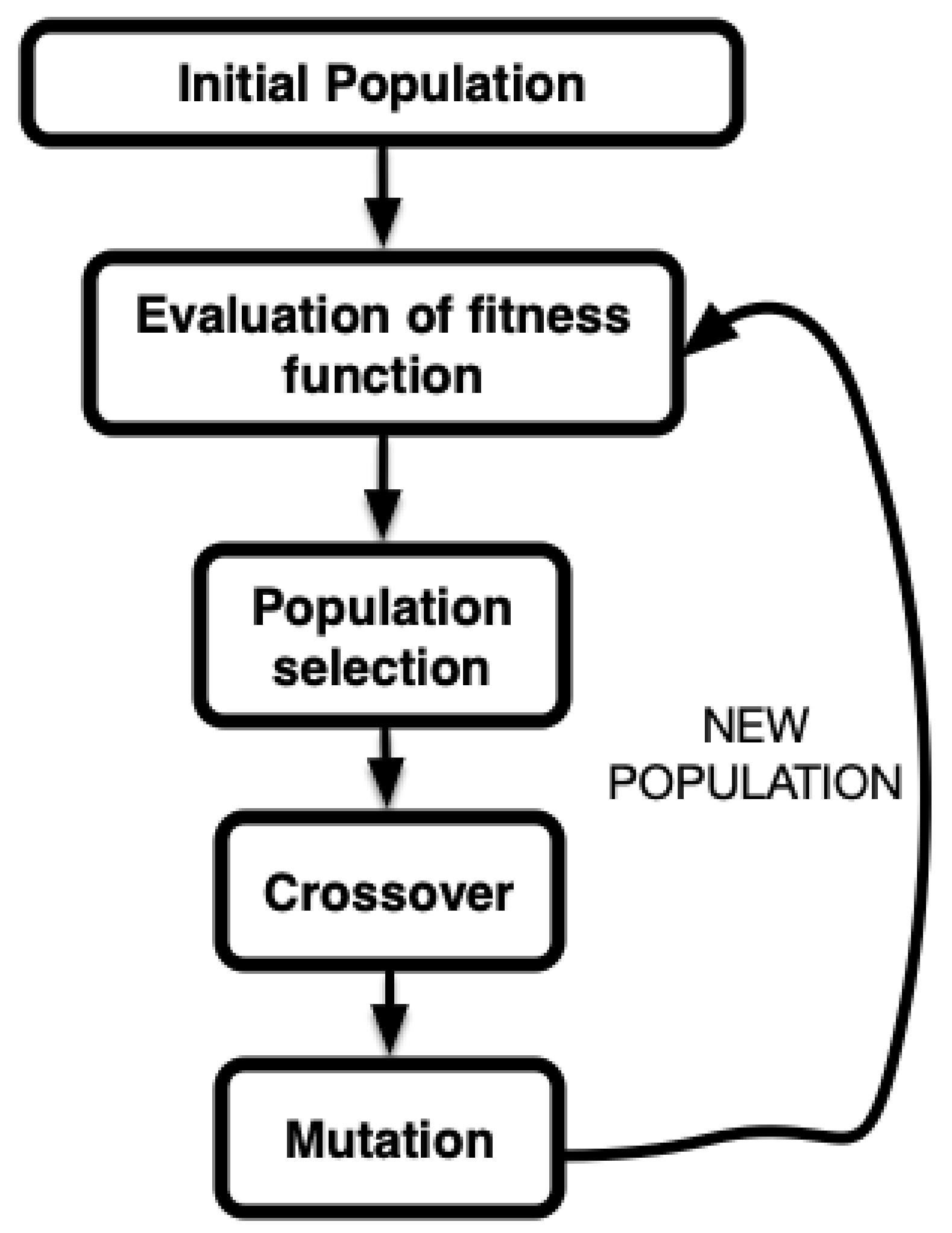
In a standard GA implementation, five phases are considered:

• Initial population: this corresponds to the initial values of the parameters with which the algorithm will start iterating.
• Fitness function calculation: the function that defines the adjustment of the parameters to the objective pursued (search for an extremum, either maximum or minimum) of a given function.
• Selection: the mechanism that establishes which elements of the population under consideration will be taken into account in the next steps of the algorithm. This stage uses the information obtained in the previous stage.
• Crossover: a way to obtain new elements in the population from the existing ones by combining the genetic information of two parents to generate a new offspring.
• Mutation: the stage of the algorithm where randomness is introduced in the elements of the population, being a key element in the search for the global extrema.

Figure 1 illustrates the aforementioned steps graphically, and Algorithm 1 provides a pseudo-code of our implementation.

Algorithm 1 Pseudo-code of the GA used

START

Generate the initial population

Compute fitness of individuals using Equation (3)

REPEAT

Selection of best fit using the Rank Selection method

Crossover using the Uniform Crossover method

Mutation using the Uniform Mutation method

Compute fitness of individuals using Equation (3)

UNTIL population has converged OR maximum number of generations reached

STOP

In the present work, we have defined each individual to be the distribution of partial pressures among each one of the possible gases. This is represented by a vector (chromosome) of 80 components (genes). A gene is represented by a real number, representing the partial pressure of one of the possible gases considered. Consequently, the GA implementation used for this optimization problem is real-valued. As mentioned earlier, partial pressures take values spanning several orders of magnitude, which can become a problem with computational methods due to the sensitivity needed for low exponent values and the range for high exponent values. Because of this, Equation (2) was used to normalize pressures so that the typical values in individuals always fall between 0 and 1 and are uniformly distributed in that interval.

The GA starts by initializing the population by generating N individuals with each one of the genes randomly initialized to a real number between 0 and 1. This is done to maximize the initial exploration space of solutions. The quality of an individual is determined by using a fitness function. In this case, a variation of MAE (mean absolute error) was used:

$$\mathrm{fitness}=-\sum _i\left|I_i-C_{ij}{P}_j\right|$$

(3)

where $I_i$ represents the normalized intensity values for the measured spectrum for mass i, $P_j$ represents the partial pressure of gas j, and $C_{ij}$ is the fragmentation pattern matrix as defined in Section 2.1. A minus sign is introduced, as GA literature suggests representing better individuals with higher fitness values [35]. The fitness values for the whole population are calculated, and the individuals are ranked accordingly. Then, a process of parent selection is carried out, in which individuals are more likely to be chosen to mate the better their rank is. This is called rank selection. A total of b individuals are chosen this way and then are allowed to mate in the hopes of obtaining an offspring of better solutions following a process of crossover and mutation.

In the crossover process, the new selected parents are divided into pairs. Two children are generated from each pair of parents. For each gene, a parent is randomly selected and the gene is directly copied from the parent to one child. The other child gets the gene from the other parent. This process is repeated for all the genes. The new children are composed of a combination of the genes from the parents, and no parent genes are lost in the process. This is referred to in literature as uniform crossover [33,35].

However, this only explores the solution space from the possibilities of the current individuals. In order to further explore the solution space, an additional process is needed: mutation, in which each gene from each one of the new individuals has a probability of $m_p$ to change its value to a uniformly distributed random number between 0 and 1. In the literature, this is referred to as uniform mutation [33,35].

The whole iterative process is repeated for $N_{gen}$ generations, and the individual with the highest fitness is the predicted result.

The final values used as hyperparameters for the GA are shown in

Table 1. Hyperparameters of the GA.

Parameter	Description	Value
N	Population size	100
b	Number of mating parents	25
$m_p$	Probability of mutation	0.03
$N_{gen}$	Number of generations	10

. They have been tuned following a grid search to achieve the best accuracy while keeping low computational times.

2.5. Reconstruction of Mass Spectra Using GAs and Gas Selection

When observing the results obtained by GAs in the reconstruction of the MS by estimating the partial pressures of 80 gases (considering all species present in our data set), we find 2 main problems to be addressed. On the one hand, optimizing 80 genes in each chromosome in the population makes the search for an optimal result very costly and time consuming. On the other hand, when all 80 gases are considered as candidates, a small value of partial pressure is found for each of them, contributing an error when calculating the weighted sum of Equation (1). Knowing that only a small number of gases are present in a typical UHV environment (usually less than 10), this could be avoided by finding an optimal initial subset of gases to be considered by the GA. Both results indicate that a pre-selection of gases is needed in order to obtain the best performance from the GAs.

As discussed in the Introduction, the considered ML model, based on classifying the presence of each gas from a probability score, is able to determine which gases are present with an accuracy >89% [2] using a probability threshold of 0.5. Thus, using this model to search for the gases to be considered in the partial pressures reconstruction seems to be a good starting point. After applying the model, the number of genes on each chromosome is significantly reduced as we restrict the search space from the initial 80 gases from the NIST 2017 database, which includes some of the most common contaminants in UHV environments [2,6], to only those detected by the ML model. Even when a threshold of 0.5 provides the best accuracy for the ML classification performed on the 80 gases, if we lower this threshold (making it less restrictive), more false positives are accepted in the pre-selected pool of candidate species. However, our hypothesis is that this will not affect the GAs negatively. Actually, it may help increase the search space by increasing the variety of parents to be crossed by the GAs, and hence increase the probability of finding a better solution, at the expense of extra computational cost.

Another aspect to be analyzed is the performance of GAs depending on the number of present gases in the vacuum system. Obviously, this has an impact on the complexity of the problem to solve and, consequently, on the convergence speeds and on the ultimate reachable reconstruction error. It is interesting to compare the results obtained in the reconstruction of the spectrum containing a variable number of gases. In our study, we analyzed the reconstruction of the MS with 2, 5 and 10 different gases, as UHV systems typically contain less than 10 contaminant species and therefore the classifier used for pre-selection was trained to simultaneously identify up to 10 distinct species [2].

We randomly generated 100 gas combinations with their respective partial pressures and corresponding MS for each one of the scenarios of study, i.e., 100 different cases for each number of gases (2, 5 and 10) and each threshold (0.5, 0.4 and 0.3) making up a total of 9 different combinations. For each one of these cases, we calculated the distribution of the integral error (IE) and its associated median. We follow the IE definition as in [8] to measure the total reconstruction error with respect to the target MS. The expression that defines the IE is the following:

$$I{E}^{norm}=\sqrt{\sum _m{(I_{calc}^{norm}-I_{gen}^{norm})}^2}$$

(4)

where $I_{calc}^{norm}$ is the calculated MS and $I_{gen}^{norm}$ is the generated MS, and both of them are transformed into the normalized logarithmic scale.

In addition, as justified in Section 2.1, it is convenient to express the mass spectrum in terms of its logarithmic expression given by Equation (2). As a consequence, GAs performed the search for the partial pressures of the gases only within the UHV range covered by this transformation. Once the partial pressures are obtained, the generated MS is built using Equation (1).

2.6. Hardware and Software

The code for this project was built using Python v3.8.5 using additional libraries NumPy v1.19.2 and Pandas v1.1.3 for data wrangling and calculations, Seaborn v0.11.0 for data visualization, and PyGAD v2.13.0 [36] as a base to implement the GA. All experiments were run using the same hardware as benchmark (Intel^® Core™ i7-10510U CPU @ 1.80 GHz x8 with 16 GB RAM).

3. Results

In

Table 2. Median of the IE distribution for each combination of threshold and number of gases.

Number of Species	Threshold
	0.5	0.4	0.3
2	0.00025	0.00021	0.00011
5	0.03423	0.02048	0.00622
10	0.42206	0.33730	0.23278

we show a summary of the medians obtained in each distribution of the IE associated with each case of study, as mentioned in Section 2.5, after 10 generations of the GA have been run.

There are two important findings related to this result. On the one hand, we note that the error increases considerably with the amount of gases we consider. On the other hand, we notice that the error decreases with the reduction of the probability threshold, which indicates that the result improves when increasing the pool of candidate gases allowed for the reconstruction of the spectrum by GAs.

Moreover, we observe how GAs work in each generation. First of all, we select the gases to be used by the search for partial pressures using the ML model [2]. Once the gases have been selected, the search for the partial pressures for each one of the gases is carried out using the GA in an iterative way, until 10 generations are reached. After each generation, the MS reconstruction is performed and compared with the real spectrum. The GA selects the spectra that provide the lowest IE. Finally, we compare the final reconstructed spectrum against the real one using Equation (4).

As shown in

Table 3. Comparison of the partial pressures (in mbar) obtained in the last iteration of the GA and the real partial pressures.

Gas Species	Predicted	Real
Benzene	$9.7\times {10}^{-09}$	$8.4\times {10}^{-09}$
Ethanol	$2.5\times {10}^{-09}$	$2.5\times {10}^{-09}$
Fluoroform	$1.9\times {10}^{-13}$	$1.1\times {10}^{-12}$
Trichloromethane	$1.7\times {10}^{-09}$	$1.9\times {10}^{-09}$
Acetaldehyde	$4.5\times {10}^{-09}$	$4.2\times {10}^{-09}$

, the predicted partial pressures for the four main gases in the sample (benzene, ethanol, trichlorometane and acetaldehyde) attain levels that are very close to the real ones, while for the fluoroform species, there is some discrepancy. The reason for this is that the first four gases have greater influence in the reconstruction of the MS, whereas the latter has a much lesser impact (note that the fitness function is the difference between the real spectrum and the reconstructed spectrum, given by Equation (3)).

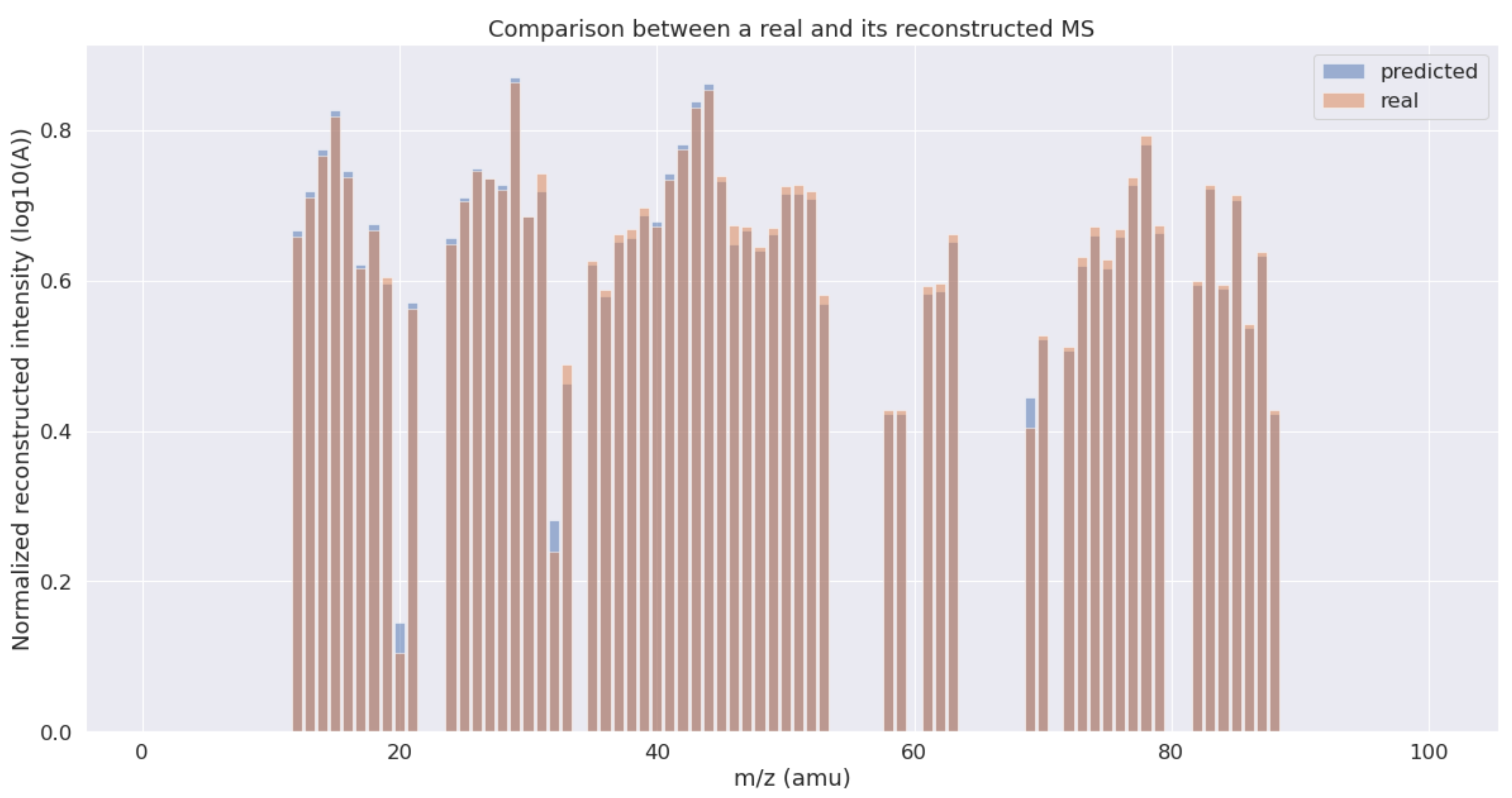
In Figure 2, we can see a comparison between the real and the reconstructed MS by the proposed method, corresponding to the gases and partial pressures shown in Table 3. As observed, the profile of the original MS is successfully reconstructed with a low error using a linear combination of the pre-selected gases weighted by the obtained partial pressures.

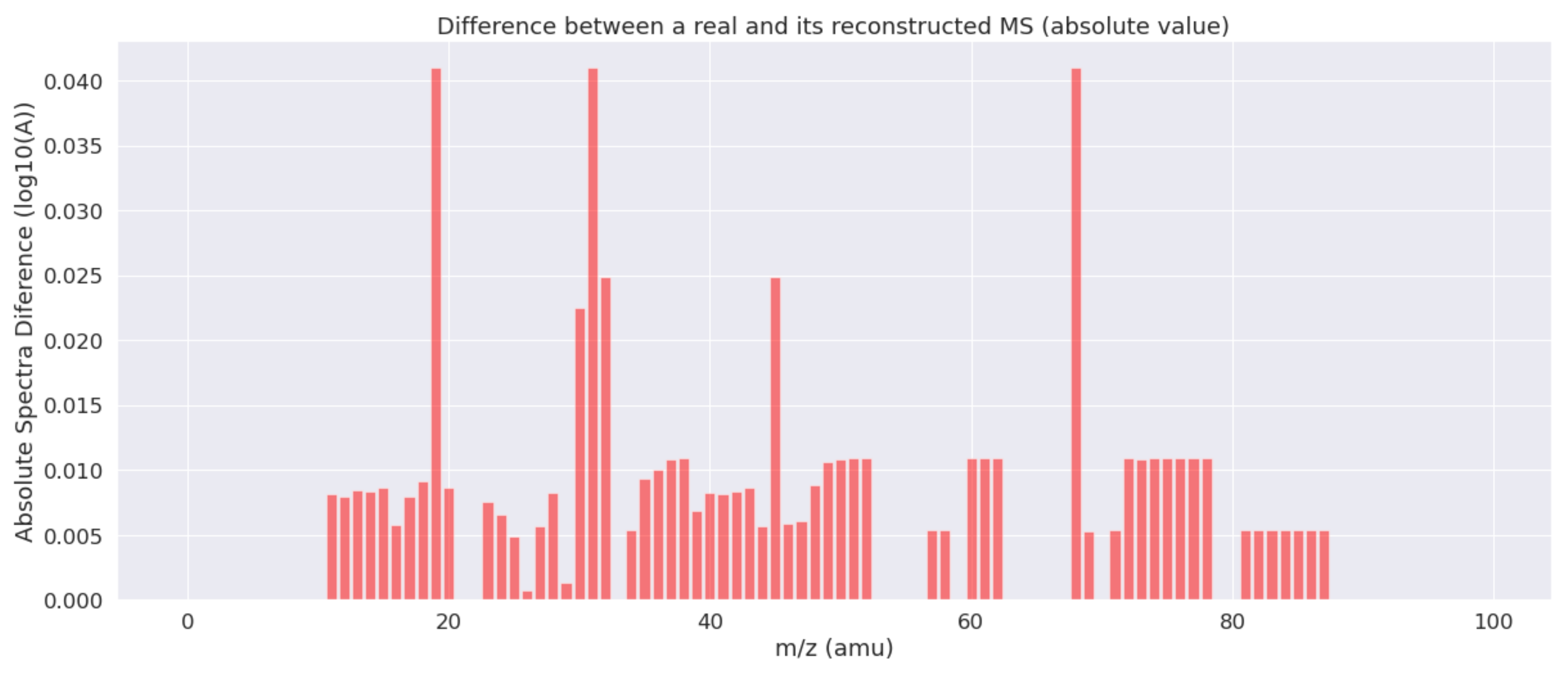
Figure 3 shows the absolute differences between both the real and the reconstructed MS of Figure 2. As can be seen, the estimated results are very close to the actual values for the majority of the mass indexes. Only in three cases, the errors are outside the confidence interval of 0.95 (considering a Gaussian distribution for the errors).

Finally, it is important to put into context the effectiveness of the model with respect to the current state of the art. As stated in Section 2.3, the technique proposed in [8] provides an estimated reconstruction based on an iterative algorithm that sequentially adds gases at their optimal pressure to the sample. This is the most advanced technique to date for solving this type of problem; it is therefore interesting to show the efficiency of our model compared to iterative deconvolution. In

Table 4. Comparison of the medians of the IE distribution obtained for the reconstruction of the MS generated with 2, 5 and 10 gases by different techniques.

Reconstruction Method	Number of Gases	Threshold
		0.5	0.4	0.3
Genetic Algorithm	2	0.00025	0.00021	0.00011
Iterative Deconvolution		0.00942	0.01293	0.01237
Genetic Algorithm	5	0.0194	0.0147	0.0108
Iterative Deconvolution		0.0818	0.0414	0.0486
Genetic Algorithm	10	0.42	0.34	0.23
Iterative Deconvolution		0.43	0.35	0.23

we compare the IE obtained by the two methods using the same pre-selection by the ML algorithm for the case of a MS containing a different number of random gases.

According to the results, for the case of the reconstruction of spectra generated by two gases, we obtain a better result from GAs for all three probability thresholds. Similarly, for the spectra generated by the combination of five gases, we also obtain a better result from GAs in all cases. However, in the case of the spectra generated with 10 gases, the results are practically identical, reaching a similar IE for both techniques. Consequently, we confirm that GAs can obtain similar or better accuracy than the iterative deconvolution technique in all of the tested scenarios.

To better interpret Table 4, in

Table 5. Approximate ratio of GA median IE values/iterative deconvolution median IE values. The best case scenarios for the GA are hightlighted in bold.

Number of Species	Threshold
	0.5	0.4	0.3
2	∼1/32	∼1/62	∼1/112
5	∼1/4	∼1/3	∼1/5
10	∼1	∼1	∼1

we present a comparison between the relative performances (IE) of both methods. We highlight in bold the most advantageous scenarios for the GA. As indicated before, the proposed method based on GA stands out specifically for lower-probability thresholds and with low-complexity spectra (composed by 2 gases). The IE reached was up to 112 times lower for the GA in the best scenario (2-gas MS and threshold = 0.3), while for a 10-gas MS, both methods behave similarly (ratio of 1).

It is also relevant to mention that the IE values obtained by GAs and those obtained by iterative deconvolution are statistically independent. Since IE medians are being compared, it is convenient to use the Wilcoxon test. This test essentially calculates the difference between sets of pairs and analyzes these differences to establish if they are significantly different from one another. The resuls of this test are presented in

Table 6. p-values resulting from the comparison between IE values of GA and iterative deconvolution using a Wilcoxon test.

Number of Species	Threshold
	0.5	0.4	0.3
2	$6.3\times {10}^{-13}$	$3.5\times {10}^{-11}$	$8.5\times {10}^{-17}$
5	$5.4\times {10}^{-10}$	$3.3\times {10}^{-12}$	$4.4\times {10}^{-11}$
10	0.04	$2.5\times {10}^{-5}$	$8.5\times {10}^{-6}$

.

All p-values are lower than 0.05, which indicates that the different sets of IE obtained by each one of the techniques used are statistically independent. This proves that both techniques behave differently and, consequently, a comparison between both methods is possible.

Once the IE results have been presented and compared, we may establish a comparison between the computational times involved by each method. A comparison between the average runtimes taken for the MS reconstruction by each method is shown in

Table 7. Ratio of iterative deconvolution runtime/GA runtime.

Number of Species	Threshold
	0.5	0.4	0.3
2	∼1	∼1.5	∼1.5
5	∼2	∼2	∼3
10	∼4	∼4	∼4

.

From Table 7, we conclude that for all two-gas scenarios, the computational time improvement is limited. However, as the number of present gases in the system is increased, we observe how the improvement in runtime of the GAs over iterative deconvolution is evident. For 5 gases, the GA takes up to 3 times less time to obtain the solution, while for 10 gases, it takes 4 times less time for any threshold scenario considered. It is also worth mentioning that, for the cases where the GA significantly improves the IE, the execution time is equal, or even less than that of the iterative deconvolution, while in the case where the IE obtained is similar, the execution time of the GA is much lower than that of the iterative deconvolution. This indicates that in all cases, the GA has a substantial advantage, either in terms of IE or in terms of computational time, compared to the iterative deconvolution.

4. Discussion

GAs have proved to be very efficient in finding extrema in multivariate functions and have been previously applied in other deconvolution problems in different research areas [16,17,18]. This led to the initial hypothesis that, given the nature of the problem exposed in this paper, these algorithms could be applied in the specific field of RGA in UHV systems.

For this research work, we created and tuned a specific GA that provided an alternative to the state of the art for identifying the contributions of the different gas species to a particular MS sample. The main findings can be summarized in the following bullet points:

• For both methods, the errors increase with the amount of candidate gases used for the construction of the real spectrum. This is a logical conclusion, as the difficulty of the problem increases with the complexity of the original MS;
• Gases contributing with very low pressures (near the detection limits used to train the classifier) are more likely produce higher relative errors, as they are penalized by the fitness function of the GA. However, these errors are very small in absolute terms and have a minimal affect in the reconstruction;
• Lowering the probability threshold for species selection helps decrease the final error reached by the GA. The reason for this is that the populations generated contain more diversity, which helps the GA get closer to the global extremum by recombining them;
• When comparing the IE obtained by the GA to the iterative deconvolution (considered a state of the art technique), we found the greatest improvement for the case of considering 2 gases and lowering the threshold to 0.3, reducing the IE by up to 2 orders of magnitude. It can also be observed that in the case of 10 gases, there is no significant improvement. This indicates that given the number of generations used in GA (10), there is an improvement limit when considering 10 gases but, for a smaller number of gases, the GA works significantly better.
• When comparing the computational times of both algorithms, the GA reaches an equal or better solution in terms of IE in the same or less time than iterative deconvolution in all cases. The computational advantage is greater the more complex the problem is, i.e., when increasing the number of gases in the original MS.

The good results obtained confirm the usefulness of GAs in this context and open up the possibility of a two-stage automatic expert system (identification of the possible gases present and approximation of the partial contributions of each one). This system optimises the process, requiring the intervention of human experts uniquely for the final stage of the process, consisting of a final review of the results. The combination of the developed expert system together with visual data mining tools will provide the UHV community with new ways to study and analyze residual gases in such environments.

It is also important to reflect on the limitations of our model when using it in a real-life scenario. In the first place, as seen in [2], the model used to identify candidate gases is trained on a subset of 80 gases from the NIST 2017 database. This obviously limits the range of gases to be found for the MS reconstruction with the GA. However, this problem could be solved by retraining the classifier to consider more gas profiles, which could be a good follow-up to this work. Secondly, the fact that the model has only been tested on simulated data limits the current possibilities of implementing it in an actual UHV environment with real data acquired from RGA. Finally, the fact that we have followed a heuristic process to adjust the threshold level could also be considered a limitation for the full automation of the reconstruction process. Future research lines include finding an efficient and automatic way to adjust this threshold.

5. Conclusions

Deconvolution and automatic MS reconstruction in UHV systems is a complex task when there are many possible contributing gas species. In this paper, we show how GAs can successfully perform the task of automatic MS reconstruction starting from a set of candidate gases selected by a multilabel classifier.

In all of the analyzed scenarios, the combined strategy that uses a ML classifier for pre-selection followed by the GA to perform the reconstruction converges to the target MS, improving the error with respect to the state of the art automatic MS reconstruction method (iterative deconvolution).

The proposed algorithm requires equal or less computational time as compared with iterative deconvolution to produce an equal or better result in all scenarios. The integral error improvement is specially noticeable for low complexity spectra and low selection thresholds, while exploring solutions with a higher number of gases greatly benefits from the efficiency of the GA in terms of speed.