Abstract
An analytical approach for the estimating of critical seismic acceleration of rock slopes was proposed in this study. Based on the 3D horn failure model, the critical seismic acceleration coefficient of rock slopes was conducted with the modified Hoek–Brown (MHB) failure criterion in the framework of upper-bound theory for the first time. The nonlinear Hoek–Brown failure criterion is incorporated into the three-dimensional rotational failure mechanism, and a generalized tangent technique is introduced and employed to convert the nonlinear Hoek–Brown failure criterion into a linear criterion. The critical seismic acceleration coefficients obtained from this study were validated by the numerical simulation results based on finite element limit analysis. The agreement showed that the proposed method is effective. Finally, design charts were provided for exceptional cases for practical use in rock engineering.
1. Introduction
Slope stability is always an important topic of debate, not only in geo-mechanics, but also in engineering practice. Many studies have adopted various failure mechanisms to analyze the slope stability issues in recent years in some theoretical methods. For example, He et al. investigated the soil slope displacement induced by the earthquake force based on the log spiral failure model proposed with considering tensile strength cut-off in upper bound theory [1,2]. Sahoo and Shukla [3] studied the stability of soil slopes incorporating the horizontal and vertical seismic loads based on the cylindrical failure model proposed by Majumdar [4] in the limit equilibrium method. It should be noted that these failure models are all plan-strain failure mechanisms. However, recent researches show that the practical slope collapse in a critical state is a three-dimensional failure, and the plane-strain failure mechanisms will lead to conservative estimations for three-dimensional slope stability issues.
Many 3D horn failure models were proposed to investigate the slope stability, e.g., 3D one-block collapse failure model, 3D multi-block mechanism, and 3D horn failure model [5,6,7]. The failure zone and stability number obtained using these analytical models were more consistent than the plane-strain failure mechanisms when compared with the experiments and numerical solutions [8]. In particular, the 3D horn failure model proposed by Michalowski and Drescher was the most prevalent failure model used to investigate slope stability [7]. The 3D horn failure model was composed of a rotation mechanism and a plane strain insert mechanism. In recent years, based on the 3D horn failure model, the effects of seepage forces, inhomogenous soils, and pile reinforcement on slope stability have been addressed [8,9,10]. Note that these researches are all limited to calculating soil slope stability numbers with the Mohr–Coulomb failure criterion. However, according to the test results [11,12,13], the strength envelops of almost all rock materials have the feature of nonlinearity. At the same time, few pieces of research incorporated the nonlinear failure criterion on the slope stability issues based on the 3D horn failure model. Moreover, even though some studies have involved the effect of seismic loads on the soil or rock slopes stability [4,9], rare researches conducted the estimation of the critical seismic acceleration of rock slopes with the modified Hoek–Brown (MHB) failure criterion. Given this, this study will fill the gaps of these researches.
In this work, the MHB failure criterion upper limit theory will be introduced to study rock slopes’ critical seismic acceleration coefficient based on the 3D rotational failure mechanism. The nonlinear Hoek–Brown failure criterion can be transformed into a linear criterion by using the generalized tangent technique. The feasibility and validity of the critical seismic acceleration coefficients obtained from this research will be verified by limit analysis based on the finite element method. Finally, a design chart will be provided for the particular situation of actual use in rock engineering.
2. MHB Failure Criterion
The Mohr–Coulomb failure criterion is a linear criterion that requires shear strength parameters cohesion c and frictional angle φ to evaluate the stability problems. Due to its simplicity, it has been widely used to investigate the stability of various geotechnical engineering for many decades [14]. However, many previous studies show that the strength of rock mass is a non-linear stress function. Therefore, the Mohr–Coulomb failure criterion could not agree well with the rock mass failure envelope, especially for the stability problems of rock slope where the rock mass is in a state of low confining stresses, making the non-linear feature more prominent.
An alternative failure criterion for the stability problem of rock mass is the MHB failure criterion involving the fitting of curves to the triaxial strength tests results of rock mass [15]. Since the MHB failure criterion was introduced, it has been widely adopted to analyze the stability of engineering structures, e.g., slope stability, strip footing stability, and tunnel stability [16,17,18]. The MHB failure criterion can be described as follows:
where and are the maximum and minimum effective principal stresses, respectively; is the uniaxial compressive stress of the intact rock. Besides, the value of , , and can be calculated by the following equations:
where denotes the Hoek–Brown constant; denotes the geological strength index; denotes the disturbance factor of the intact rock. Hence, for the MHB failure criterion, there is a total of four input parameters, namely,, , , and . These four material parameters for the MHB failure criterion could be obtained directly from Priest [19].
The generalized tangential technique conducted by Yang et al. was adopted to transform the nonlinear criterion into a linear one to estimate the tunnel stability by the MHB failure criterion in this study, shown in Figure 1 [16]. It can be concluded that the tangential line technique could provide an upper-bound solution for the stability issues due to the tangential line exceeding the original non-linear envelope. The tangential line at point M could be expressed as the following classic equation:
where and are the tangential cohesion and tangential friction angle, respectively; can be calculated as follows:
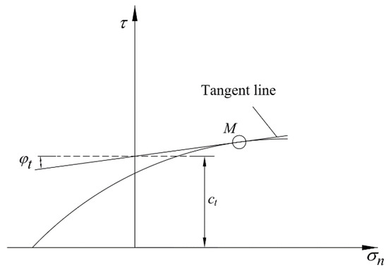
Figure 1.
Tangential line to the modified Hoek–Brown (MHB) yield criterion.
In Equation (6), the tangential cohesion is the mutative parameter with the change of internal friction angle .
3. Problem Statements
Figure 2 presents the stability issue of the slope with the MHB failure criterion. The geometry of the studied problem was denoted by the slope height H and the slope angle β. In order to make the applicability of the calculation results more transparent, the following assumptions were adopted:
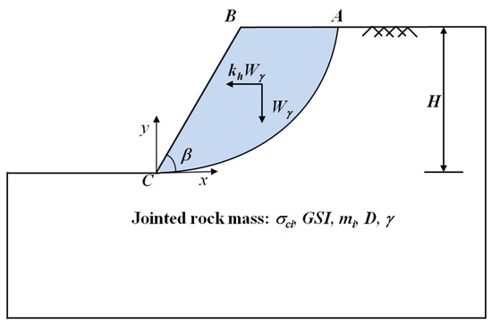
Figure 2.
Simplified model for a rock mass slope. Point A and C are the end points of the sliding surface; H is the slope height; β is the slope angle; is the horizontal seismic acceleration coefficient; and is the work rate of the rock weight.
(1) The ground surfaces were assumed to be horizontal, and the impact of pore water pressure was not considered in this work.
(2) The failure model was presumed as a rotational body around the same axis through O with the same angular velocity ω.
(3) The influence of seismic loads is assumed as a horizontal force acting on the failure model.
The third assumption is the classical pseudo-static approach, which has been widely used to conduct the seismic stability assessment of slopes with linear Mohr–Coulomb failure criterion [20,21].
4. 3D Horn Failure Model
To assess the slope stability, many researchers have proposed various failure mechanisms, such as the log spiral failure model and cylindrical failure model [1,3,4]. It should be noted that these failure models were all plan-strain failure mechanisms. However, recent published literatures showed that the practical collapse of slopes in the critical state is a three-dimensional failure, and the plan-strain failure model will definitely result in conservative (unsafe) estimations for three-dimensional slope stability issues. To solve this shortcoming, Michalowski developed a 3D rotational failure mechanism that had the shape of a curvilinear cone with an apex angle (see Figure 3 and Figure 4) [6]. Figure 3 presented the longitudinal section of the 3D horn failure model. Figure 4 presented the cross-section of the 3D horn failure model. It can be seen in Figure 4 that the 3D horn failure model was composed of two parts: (1) the plane-strain insert; and (2) the 3D horn section. The plane-strain insert had the geometry of the logarithmic spiral and connected the two 3D horn sections, which allowed a transition to the plane-strain case if there is no limitation to the slope width. The 3D horn section was the end part of the failure mechanism. The 3D horn failure model was bounded by two log-spirals (see Figure 3) by respecting normality rule:
where, and (see Figure 3). A detailed description of the 3D horn failure model could be found in Michalowski’s study. In the light of the study, the 3D horn failure model had been repetitively adopted in the estimation of the slope stability. The effects of pore water pressure, inhomogeneous soils, pile reinforcement and seismic loads on the slope stability in the linear Mohr–Coulomb failure criterion were investigated, respectively [8,9,10]. However, rare research had estimated critical seismic acceleration of rock slopes using the 3D horn failure model in the MHB failure criterion. Consequently, this study will fill this gap.
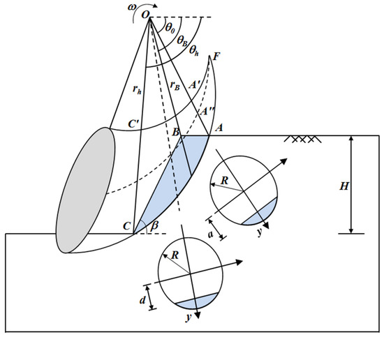
Figure 3.
Longitudinal section of the 3D horn failure model.

Figure 4.
3D horn failure model with plane insert.
5. Critical Seismic Acceleration Based on the Upper Bound Theory
In the framework of the upper bound theorem, the critical seismic acceleration was obtained by equating the total energy dissipation rate to the total work rate of external forces, which was as follows:
where D denotes the energy dissipation rate, denotes the rate of work of the rock weight, and is the rate of work done by seismic loads.
5.1. Work Rate of the Internal Energy Dissipation
From Figure 3, it can be seen that the energy dissipation rate consists of two parts and can be expressed as:
where, and respectively denote the energy dissipation rate in the plane strain insert part and the 3D horn part. The detailed derivation of the energy dissipation rate could be described as follows.
(1) Calculation of
The expression of can be described as follows:
where, and ; β is the slope angle; is the tangential cohesion and can be obtained from Equation (6); is the tangential frictional angle (see Figure 2), and it was an optimal parameter in this study; , , and could be found in Figure 3.
(2) Calculation of
The expression of can be described as follows:
where, denotes the width of the plane insert failure part (see Figure 4).
5.2. Work Rate of the Rock Weight
From Figure 3, it can be seen that the rate of work of the rock weight consisted of two parts and can be expressed as:
where, and respectively denote the rate of work of the rock weight for the plane strain insert part and the 3D horn part. The detailed derivation of the rate of work of the rock weight could be described as follows.
(1) Calculation of
The expression of can be described as follows:
where, .
According to the geometrical relations, a and b could be expressed as:
where, and .
(2) Calculation of
The expression of can be described as follows:
with
where,
5.3. Work Rate of the Seismic Loads
In this work, the pseudo-static approach was adopted to incorporate the impact of seismic forces into the 3D horn failure model. Because the vertical seismic acceleration had little influence on seismic displacements of slopes [21], the vertical seismic acceleration was not considered in this study. From Figure 3, the rate of work done by the seismic loads could be divided into two parts and could be expressed as:
where, and respectively denotes the rate of work of seismic loads for the plane strain insert part and 3D horn part. The detailed derivation of the rate of work done by the seismic loads could be described as follows:
(1) Calculation of
Combining Equation (14) and Figure 3, the expression of can be described as:
where, denotes the horizontal seismic acceleration coefficient and could be obtained by the following equation:
where, is the horizontal seismic acceleration, and is the gravity acceleration.
(2) Calculation of
5.4. Calculation of Critical Seismic Acceleration
Combining the Equations (9)–(27), the critical seismic acceleration coefficient could be obtained by equating the energy dissipation rate to the total rate of work of external forces based on upper-bound limit analysis theory as follows:
It should be noted that the critical seismic acceleration coefficient obtained in this work was the minimum of Equation (28) with respect to , with given constraint MHB parameters (,,,, ) and slope geometry (,), with the aid of the optimization tool (particles warm) in Matlab.
From Equation (28), when the values of material parameters (,,,) are given, one could easily find that the critical seismic acceleration coefficient was uniquely related to the slope geometry (), which could be presented in Equation (29).
A dimensionless parameter SR was defined in this study as follows:
Then Equation (29) can be substituted by Equation (31),
Four different groups of critical seismic acceleration coefficient with different parameters but the same are presented in Table 1. From Table 1, the values of the critical seismic acceleration coefficient kept constant for the cases of the same , which indicated that the was uniquely related to the dimensionless parameter , regardless of the magnitude of individual parameters .

Table 1.
Comparison of the of given rock slopes with the same SR. SR is a dimensionless parameter defined in Equation (30); mi is the Hoek–Brown constant; GSI is the geological strength index; Di is the disturbance factor of the intact rock; β is the slope angle; σci is the uniaxial compressive stress of the intact rock; γ is the unit rock weight; H is the slope height; khc is the critical seismic acceleration coefficient.
6. Validation
Since no theoretical models have estimated rock slopes’ critical seismic acceleration coefficient in the MHB failure criterion, a numerical simulation using finite element limit analysis (FELA) was adopted here to validate the proposed method. A recent study showed that FELA can be adopted to accurately evaluate the seismic stability of slopes by combining with the pseudo-static approach [21]. It should be noted that FELA was a 2D numerical simulation software, which had been widely used to study the stability issues of various engineering structures [18,21,22]. Due to the 2D analysis neglecting the influence of the energy dissipation rate done by horn failure part (see Figure 4), the results obtained from 2D analysis are more conservative when compared with those from 3D analysis [7,9]. Recent works also showed that the results for B/H = +∞ can be regarded as the 2D solutions [7,23]. Figure 5 shows the critical seismic acceleration coefficients khc calculated in this work compared with those calculated by FELA for = 45°, GSI = 30, = 0.5, and = 10. It is worth noting that, in Figure 5, SR is a defined dimensionless parameter, and can be calculated by using Equation (30).
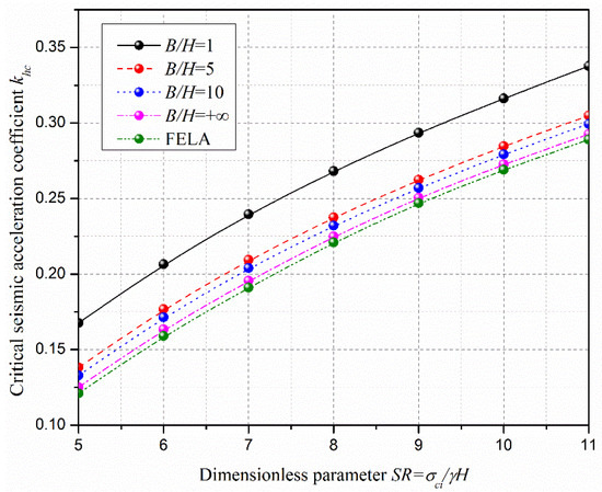
Figure 5.
Comparison between the results from this work and finite element limit analysis FELA.
From Figure 5, it could be seen that both SR and B/H had a significant influence on the critical seismic acceleration coefficient . As also shown in Figure 5, one could conclude that the values of the critical seismic acceleration coefficient calculated in this work for B/H = +∞ were slightly higher than those from FELA, with the most significant ratio less than 3.5%, which illustrates the validity of the proposed method. It can also be seen in Figure 5 that the gap between the results from this study and FELA increased with the B/H decrease, due to the FELA is a 2D numerical simulation software, which indicated that it would lead to conservative estimations for stability of three-dimensional slope, especially for narrow slopes. The similar conclusions can be found in Yang et al. [23] and Michalowski and Drescher [7]. These observations illustrated that the proposed method could be used to accurately determine the critical seismic acceleration coefficient for 3D rock slopes.
7. Results and Discussion
In this section, the effects of B/H, SR, and on the critical seismic acceleration coefficient were presented and discussed in the distributed and undistributed rock slopes. Table 2 shows the critical seismic acceleration coefficient calculated in this work for the cases of GSI = 20, = 7 and = 0. Table 3 shows the critical seismic acceleration coefficient calculated in this study for the cases of GSI = 30, = 10 and = 0.5. From Table 2 and Table 3, it could be clearly seen that the B/H, SR, and all had great significance on the critical seismic acceleration coefficient . The critical seismic acceleration coefficient decreased with the increasing of B/H and , and increased with SR.
Table 2.
Critical seismic acceleration coefficient for GSI = 20, = 7 and = 0.
Table 3.
Critical seismic acceleration coefficient for GSI = 30, = 10 and = 0.5.
8. Conclusions
Based on the 3D horn failure model, the critical seismic acceleration coefficient was determined using upper-bound limit analysis theory with the MHB failure criterion. The generalized tangential technical was adopted to transfer the MHB failure criterion to a linear one. Based on the obtained results, the following conclusions can be drawn:
1. Based on the generalized tangential technical, the MHB failure criterion was adopted to estimate the stability of rock slopes. The comparisons between the results from this study and FELA showed that the generalized tangential technical could be accurately used to evaluate the stability issues of rock slopes with the MHB failure criterion.
2. Based on the 3D horn failure model, the critical seismic acceleration coefficient was determined with the MHB failure criterion. The results showed that all parameters have a great influence on the critical seismic acceleration coefficient. Previously, researchers tended to focus on estimating the stability number of slopes and rarely calculated the critical seismic acceleration coefficient, especially for the MHB failure criterion.
3. Even though the critical seismic acceleration coefficient of rock slopes was conducted based on the 3D horn failure model with the MHB failure criterion in this work, a possible extension of this work could be further investigated to determine the displacement of rocks slopes induced by seismic loads by considering the earthquake duration, arias energy, etc., and with a combination of probabilistic approaches.
Author Contributions
Conceptualization, Q.M. and X.H.; methodology, G.C.; software, P.L. and Z.W.; validation, Q.M. and X.H.; writing—original draft preparation, Q.M.; writing—review and editing, X.H. All authors have read and agreed to the published version of the manuscript.
Funding
This research was funded by the Huxiang Young Talent Project, grant number [2020RC3090].
Institutional Review Board Statement
Not applicable.
Informed Consent Statement
Not applicable.
Data Availability Statement
Not applicable.
Conflicts of Interest
The authors declare no conflict of interest.
References
- He, Y.; Liu, Y.; Hazarika, H.; Yuan, R. Stability analysis of seismic slopes with tensile strength cut-off. Comput. Geotech. 2019, 112, 245–256. [Google Scholar]
- Meyerhof, G.G.; Chen, W.F. Limit Analysis and Soil Plasticity (1975) elsevier, amsterdam 638 dfl. 240.00. Eng. Geol. 1976, 10, 79. [Google Scholar] [CrossRef]
- Sahoo, P.P.; Shukla, S.K. Taylor’s slope stability chart for combined effects of horizontal and vertical seismic coefficients. Géotechnique 2019, 69, 344–354. [Google Scholar]
- Majumdar, D.K. Stability of Soil Slopes under Horizontal Earthquake Force. Géotechnique 1971, 21, 84–88. [Google Scholar] [CrossRef]
- Shi, H.; Chen, G. Relationship between critical seismic acceleration coefficient and static factor of safety of 3D slopes. J. Cent. South. Univ. 2021, 28, 1546–1554. [Google Scholar] [CrossRef]
- Michalowski, R.L. Three-dimensional analysis of locally loaded slopes. Geotechnique 1989, 39, 27–38. [Google Scholar] [CrossRef]
- Michalowski, R.L.; Drescher, A. Three-dimensional stability of slopes and excavations. Géotechnique 2009, 59, 839–850. [Google Scholar] [CrossRef]
- Pan, Q.; Dias, D.; Jingshu, X.U. Three-Dimensional stability of a slope subjected to seepage forces. Int. J. Geomech. 2017, 17, 04017035. [Google Scholar] [CrossRef]
- Yang, X.L.; Xu, J.S. Three-Dimensional Stability of Two-Stage Slope in Inhomogeneous Soils. Int. J. Geomech. 2016, 17, 06016045. [Google Scholar] [CrossRef]
- He, Y.; Hazarika, H.; Yasufuku, N.; Han, Z.; Li, Y. Three-dimensional limit analysis of seismic dis-placement of slope reinforced with piles. Soil Dyn. Earthq. Eng. 2015, 77, 446–452. [Google Scholar] [CrossRef]
- Baker, R. Nonlinear Mohr Envelopes Based on Triaxial Data. J. Geotech. Geoenvironmental Eng. 2004, 130, 498–506. [Google Scholar] [CrossRef]
- Cai, M.; Kaiser, P.K.; Tasaka, Y.; Minami, M. Determination of residual strength parameters of jointed rock masses using the GSI system. Int. J. Rock Mech. Min. Sci. 2007, 44, 247–265. [Google Scholar] [CrossRef]
- Serrano, A.; Olalla, C. Discussion of “Nonlinear Mohr Envelopes Based on Triaxial Data” by R. Baker. J. Geotech. Geoenvironmental Eng. 2006, 132, 128–129. [Google Scholar] [CrossRef]
- Li, P.; Wang, F.; Zhang, C.; Li, Z. Face stability analysis of a shallow tunnel in the saturated and multi-layered soils in short-term condition. Comput. Geotech. 2018, 107, 25–35. [Google Scholar] [CrossRef]
- Kulatilake, P.H.S.W.; Shu, B. Prediction of Rock Mass Deformations in Three Dimensions for a Part of an Open Pit Mine and Comparison with Field Deformation Monitoring Data. Geotech. Geol. Eng. 2015, 33, 1551–1568. [Google Scholar] [CrossRef]
- Yang, X.L.; Li, L.; Yin, J.H. Seismic and static stability analysis for rock slopes by a kinematical approach. Geotech. 2004, 54, 543–549. [Google Scholar] [CrossRef]
- Yang, L.X.; Yin, J.H. Upper bound solution for ultimate bearing capacity with a modified Hoek–Brown failure criterion. Int. J. Rock Mech. Min. Sci. 2005, 42, 550–560. [Google Scholar] [CrossRef]
- Zhang, R.; Chen, G.; Zou, J.; Zhao, L.; Jiang, C. Study on roof collapse of deep circular cavities in jointed rock masses using adaptive finite element limit analysis. Comput. Geotech. 2019, 111, 42–55. [Google Scholar] [CrossRef]
- Priest, S.D. Determination of Shear Strength and Three-dimensional Yield Strength for the Hoek-Brown Criterion. Rock Mech. Rock Eng. 2005, 38, 299–327. [Google Scholar] [CrossRef]
- Chen, G.H.; Zou, J.F.; Pan, Q.J.; Qian, Z.H.; Shi, H.Y. Earthquake-induced slope displacements in heterogeneous soils with tensile strength cut-off. Comput. Geotech. 2020, 124, 103637. [Google Scholar] [CrossRef]
- Peng, W.; Zhao, M.; Zhao, H.; Yang, C. Seismic Stability of the Slope Containing a Laterally Loaded Pile by Finite-Element Limit Analysis. Int. J. Geomech. 2022, 22, 06021033. [Google Scholar] [CrossRef]
- Chen, G.; Zou, J.; Zhang, R. Stability analysis of rock slopes using strength reduction adaptive finite element limit analysis. Struct. Eng. Mech. 2021, 79, 487–498. [Google Scholar]
- Yang, T.; Zou, J.; Pan, Q. Three-dimensional seismic stability of slopes reinforced by soil nails. Comput. Geotech. 2020, 127, 103768. [Google Scholar] [CrossRef]
Publisher’s Note: MDPI stays neutral with regard to jurisdictional claims in published maps and institutional affiliations. |
© 2021 by the authors. Licensee MDPI, Basel, Switzerland. This article is an open access article distributed under the terms and conditions of the Creative Commons Attribution (CC BY) license (https://creativecommons.org/licenses/by/4.0/).