Analysis of Storage Effects in the Recirculation Zone Based on the Junction Angle of Channel Confluence

Abstract

In this study, numerical simulations using the Environmental Fluid Dynamics Code model were conducted to elucidate the effects of flow structures in the recirculation zone on solute storage based on the junction angle. Numerical simulations were performed at a junction angle of 30° to 90° with a momentum flux ratio of 1.62. The simulation results revealed that an increase in the junction angle caused the recirculation zone length and width to increase and strengthened the development of helical motion. The helical motion increased the vertical gradient of the mixing layer and the mixing metric of the dosage curves. The recirculation zone accumulated the solute as a storage zone, which formed a long tail in the concentration curves. The interaction between the helical motion and recirculation zone affected the transverse mixing, such that the transverse dispersion had a positive relationship with the helical motion intensity and a negative relationship with the recirculation zone size. Transverse mixing exhibited an inverse relationship with the mass exchange rate of the recirculation zone. These results indicate that the transverse dispersion is replaced by mixing due to strongly developed storage zones.

1. Introduction

The prediction of mixing characteristics of solute inputs in rivers affects decision-making management in the operation of hydraulic structures for the safety of local residents. Solute mixing caused by shear flow is commonly analyzed using the advection–dispersion equation based on Fick’s law [1]. However, the complex topography of rivers and hydraulic structures such as dams and weirs generates storage zones that induce non-Fickian mixing [2]. Storage zones in rivers mainly consist of surface transient storage in recirculation zones and hyporheic transient storage [3]. Previously, many researchers have used a one-dimensional (1D) storage model to simulate the mixing phenomena in these types of storage zones [4,5,6]. To increase the accuracy of these storage zone models, determination of the model parameters is important. Therefore, many previous studies have conducted parameter calibrations using concentration curves obtained from tracer experiments [7,8,9,10]. However, these calibrated parameters are associated with high uncertainties because the three-dimensional (3D) characteristics of solute mixing in actual tracer tests are translated into results for 1D storage model parameter values.

The inflow of tributaries into main channels is one of the main sources of solute transport. Therefore, analysis of tributary mixing characteristics is important for water quality management. Jung et al. [11] conducted field studies on river confluences to prove that the discharge ratio of the main and tributary channels changes the secondary current intensity, which affects solute transverse mixing. This demonstrates the relevance of the flow characteristics between tributaries and main channels to near-field mixing analysis in confluences. Figure 1 presents a conceptual image of the flow and solute mixing characteristics near a channel confluence. In the channel confluence, a shear layer is formed and a recirculation zone is developed by the decrease in pressure on the inner side of the confluence [12], as shown in Figure 1. A circular motion is formed as a result of discharge from the tributary channel at the outer side of the confluence. The complex characteristics of the flow in the confluence change with the junction angle, discharge ratio between the main and tributary flows, discordance of the channel bed at the entrance to the confluence, geometric symmetry, density contrasts, and potentially, the width–depth ratio [13,14,15,16]. Research on the analysis of flow characteristics in confluences has been conducted based on field measurements, experimental research, and numerical simulations. Schindfessel et al. [17] demonstrated that turbulent kinetic energy increased with an increase in the tributary discharge in the mixing layer developed in the recirculation zone. Yuan et al. [18] reported that helical motion became stronger and elongated when the tributary discharge was greater than the discharge of the main channel. Gualtieri et al. [19] demonstrated that the momentum transfers and the mixing interface width in the confluence hydrodynamic zone depend on the flow conditions. Yuan et al. [20] conducted analysis of the helical motion in confluences and found that flow structures originating from circular cells affect sediment transport. Other researchers have conducted numerical simulations using the Reynolds-Averaged Navier–Stokes (RANS) model to analyze 3D flow characteristics based on field measurements and laboratory experiments [21,22,23,24,25]. Additionally, detailed turbulence structures in the mixing interfaces of confluences have been analyzed through detached eddy simulations using the RANS model [26,27,28,29].

The junction angle influences near-field mixing by creating a recirculation zone and helical cells downstream of the confluence. Near-field mixing at confluences can be divided into rapid mixing, where transverse mixing is completed within a short distance, and slow mixing, where transverse mixing is maintained further downstream [30]. Lane et al. [31] found that the presence of channel-scale circulation at a confluence transforms slow mixing into rapid mixing. Rapid mixing occurs when a tributary flow flows into a main channel with a large junction angle. In such cases, a difference in concentration between the main and tributary channel creates a mixing interface in which the vertical gradient is increased, leading to the stimulation of vertical mixing and rapid completion of transverse mixing. In this context, Ramón et al. [14] stated that the momentum flux ratio and junction angle are important hydraulic factors that influence the location of the mixing interface. Furthermore, weak density contrast at the confluence increases the mixing area by distorting the mixing interface, leading to an increase in transverse mixing [32]. The effect of density contrast on mixing is more dominant farther downstream from the confluence than differences in the velocity of the main and tributary channel [33]. Lewis et al. [16] demonstrated that a tributary flow with strong momentum flux induces helical motion, which moves the mixing interface toward the outer bank, causing transverse mixing to increase. The strong momentum flux affects not only the helical motion but also the flow separation, which causes solute storage. Constantinescu et al. [26] demonstrated that strong Kelvin–Helmholtz instabilities induce vortex pairing in the mixing layer in the recirculation zone, which causes sediment to be actively mixed in the recirculation zone. Despite several studies related to mixing in confluences, it is still difficult to define the effects of storage zones induced by the recirculating flow in confluences on transverse dispersion.

The goal of this study was to analyze the effects of recirculation zones in channel confluences on solute storage. This research focused on the influence of the confluence angle on solute mixing and associated storage effects. The flow structure at a confluence and its effects on solute mixing were simulated using the quasi-three-dimensional model Environmental Fluid Dynamics Code (EFDC). The EFDC model has been used frequently in many riverine, estuary, flow, and solute mixing simulations, and it has been proven to be reasonably accurate [34,35,36,37]. The EFDC was applied to various junction angles to determine their effect on the size of the recirculation zone. An analysis of solute mixing through helical motion and recirculation zones was also conducted. Additionally, the retention time changes of solutes caused by junction angle changes were investigated based on the results of mixing characteristics in confluences.

2. Methods and Background

2.1. Flow and Mixing Characteristics at a Confluence

2.1.1. Separation and Recirculation Zone Downstream of a Confluence

The momentum flux in a tributary channel may cause the flow to detach as it joins the main channel, creating a recirculation zone as a result of low pressure. When two water bodies with the same density are combined into one, the momentum flux ratio is calculated using the following equation:

$$M_r=\frac{Q_t{U}_t}{Q_m{U}_m}$$

(1)

where $M_r$ is the momentum flux ratio, $Q_m$ and $Q_t$ are the flow rates of the main and tributary channels, respectively, and $U_m$ and $U_t$ are the cross-sectional averaged velocities of the main and tributary channels, respectively. As the momentum ratio and discharge ratio increase, the width and length of the recirculation zone also increase, and the recirculation zone range is affected by junction angle changes.

The length and width of the recirculation zone can be predicted based on the discharge ratio between the main and tributary channels, as well as the junction angle. Gurram et al. [38] presented an empirical formula to calculate the width and length of a recirculation zone based on experimental results. The recirculation zone characteristics for subcritical flow can be estimated according to the junction angle as

$$\frac{L_s}{W}=3.8{ \sin }^3\alpha \left(1-\frac{1}{2}{\mathrm{Fr}}_d\right)Q_r^{1/2}$$

(2)

$$\frac{b_s}{W}=\frac{1}{2}{\left({\mathrm{Fr}}_d-\frac{2}{3}\right)}^2+0.45Q_r^{1/2}\left(\frac{\alpha }{{90}^{\circ }}\right)$$

(3)

where $L_s$ and $b_s$ are the length and width of the recirculation zone, respectively, as depicted in Figure 1, $\alpha$ is the junction angle, $Q_r$ is the discharge ratio defined as $Q_m/\left(Q_m+Q_t\right)$, and ${\mathrm{Fr}}_d$ is the Froude number downstream of the confluence defined as $U/\sqrt{g{h}_0}$ in which $U$ is the cross-sectional averaged velocity and $h_0$ is the downstream water depth. The recirculation zone becomes a storage zone for solutes and affects the mixing characteristics downstream of the junction [26]. Therefore, the accurate prediction of the size of the recirculation zone is important.

2.1.2. Transverse Mixing at a Confluence

Under high-momentum-flux-ratio conditions, the shear plane caused by tributary inflows induces helical motion, as shown in Figure 1. This helical motion influences transverse mixing in confluences, which can be divided into slow mixing or rapid mixing according to the hydraulic characteristics. The width of a solute cloud can be defined as six times the standard deviation of a concentration curve under the assumption of the Fickian mixing [39]. When the concentration changes are less than 5% throughout the channel width, transverse mixing is considered to be complete [40]. When the distance between the solute input source and transverse mixing completion point ($L_m$) is five to 10 times the width of the channel, it is considered to be rapid mixing [30]. In the case of slow mixing, the distance between the source and completion point is 100 times the channel width [31,41]. The transverse concentration changes caused by tributary inflows can be evaluated using a standard deviation defined as

$${\sigma }_r=\frac{{\sigma }_{ds}}{{\sigma }_{us}}$$

(4)

where ${\sigma }_r$ is the dimensionless mixing metric, and ${\sigma }_{us}$ and ${\sigma }_{ds}$ are the standard deviations of transverse concentration variations in the upstream and downstream cross-sections, respectively. If the value of ${\sigma }_r$ is one, then the concentration changes throughout the upstream and downstream widths of the channel are the same, and transverse mixing does not occur. In contrast, if the value of ${\sigma }_r$ is zero, then transverse mixing is considered to be complete [41].

For a transient solute input from a tributary, transverse mixing can be analyzed by integrating time-varying concentration curves over time and converting them into steady-state conditions. The dosage curve is the time-integrated value of the concentration passing through one point, which can be calculated using the following equations [42]:

$$\theta ={\displaystyle {\int }_0^{\infty }C\left(x, y, t\right)dt}$$

(5)

$$\Theta ={\displaystyle {\int }_0^1\theta \left(x, \eta \right)d\eta }$$

(6)

$$\eta =\frac{{\displaystyle {\int }_0^y\sqrt{{\overline{u}}^2+{\overline{v}}^2}hdy}}{Q}=\frac{q}{Q}$$

(7)

where $\theta$ is the time integration of the concentration passing a point, $C$ is the depth-averaged concentration, $\mathrm{\Theta }$ is the total dosage in a cross-section, $\eta$ is the dimensionless cumulative discharge, $\overline{u}$ and $\overline{v}$ are the depth-averaged velocity in the x and y-direction, respectively, $q$ is the cumulative discharge, and $h$ is the water depth. The transverse dispersion coefficient can be estimated from the dosage curves shown in Equation (5) using the moment method as

$$D_T=\frac{U}{2}\frac{d{\sigma }_{\theta }^2}{dx}$$

(8)

$${\sigma }_{\theta }^2=\frac{{\displaystyle {\int }_0^W\theta y^2}dy}{{\displaystyle {\int }_0^W\theta }dy}$$

(9)

where $D_T$ is the transverse dispersion coefficient, ${\sigma }_{\theta }^2$ is the variance of the dosage curves, and $W$ is the channel width.

The recirculating flow in a confluence can form a storage zone that traps the solute inflow from a tributary. Such a storage zone increases the residence time of solutes and generates a long-tailed concentration curve [43]. The mixing characteristics in rivers change as a result of these storage zones, which affects far-field mixing results. Therefore, many studies have adopted the following storage model to analyze far-field mixing considering storage zones [44]:

$$\frac{\partial C_f}{\partial t}+U\frac{\partial C_f}{\partial x}=K_f\frac{{\partial }^2{C}_f}{\partial x^2}+\frac{\epsilon }{T}\left(C_s-C_f\right)$$

(10)

$$\frac{\partial C_s}{\partial t}=\frac{1}{T}\left(C_f-C_s\right)$$

(11)

$$T=\frac{A_s}{kP}$$

(12)

where $C_f$ and $C_s$ are the concentrations in the flow and storage zones, respectively, $K_f$ is the longitudinal dispersion coefficient for the flow zone, $\epsilon =A_s/A$, $A_s$ is the cross-section area of the recirculation zone, $A$ is the entire flow area, $k$ is the mass exchange coefficient, $P$ is the boundary length between flow and recirculation zone, and $T$ is the residence time in the storage zone. After a solute has been trapped in the recirculation zone for a sufficient amount of time, the concentration of the flow zone ($C_f=0$) becomes zero, and the following equation can be derived [6]:

$$\ln \left(\frac{C_s}{C_{s0}}\right)=-\frac{t}{T}$$

(13)

where $C_{s0}$ is the initial concentration in the storage zone. By using Equation (13), the parameters for the storage zone model can be estimated by analyzing changes in the solute concentration–time curves in the recirculation zone.

2.2. Model Descriptions and Grid Sensitivity Analysis

2.2.1. Descriptions of EFDC

The hydrodynamic module of the EFDC includes quasi-3D flow analysis and solute transport models. The flow analysis model adopts the RANS equation as a governing equation that considers hydrostatic pressure instead of solving the vertical momentum equation [45]. Although this hydrostatic pressure assumption is limited in terms of reproducing vertical flow, this model, with its quasi-three-dimensional characteristics, was determined to be appropriate for this type of research, even though confluences have vertical flow. This flow analysis model adopts the Smagorinsky model [46] and the Mellor–Yamada 2.5 model [47] as turbulence closure methods for estimating the horizontal and vertical eddy viscosities, respectively. The model solves the governing equations using a combination of finite volume and finite difference scheme on an orthogonal curvilinear coordinate system in the horizontal direction. In the vertical direction, the equations are transformed using the sigma coordinate system. The model employs the mode splitting method, which separates the computation into external and internal mode. In the external mode, free surface elevation is obtained from the depth-averaged governing equations. In the internal mode, velocity shear is computed using the results by the external mode. More details about the numerical formulations can be found in Hamrick [45].

The solute transport model is coupled with the flow analysis model, and the governing equation of the solute transport model is given as

$$\begin{array}{ll}\frac{\partial }{\partial t}\left(m_x{m}_{y}Hc\right)& +\frac{\partial }{\partial x}\left(m_{y}Huc\right)+\frac{\partial }{\partial y}\left(m_{x}Hvc\right)+\frac{\partial }{\partial z}\left(m_x{m}_{y}wc\right)\\ & =\frac{\partial }{\partial x}\left(\frac{m_y}{m_x}H{\epsilon }_h\frac{\partial c}{\partial x}\right)+\frac{\partial }{\partial y}\left(\frac{m_x}{m_y}H{\epsilon }_h\frac{\partial c}{\partial y}\right)+\frac{\partial }{\partial z}\left(m_x{m}_y\frac{{\epsilon }_z}{H}\frac{\partial c}{\partial z}\right)\end{array}$$

(14)

where $c$ is the time-averaged concentration, $m_x$ and $m_y$ are the metric coefficients, $H=\zeta +h$, $\zeta$ is the bottom elevation, and ${\epsilon }_h$ and ${\epsilon }_z$ are the horizontal and vertical turbulent diffusion coefficient, respectively. The turbulent diffusion coefficients in Equation (14) are considered as the eddy viscosity according to the Reynolds analogy [40], which has been adopted for simulations without density differences between the main and tributary channels [48,49]. However, it has been reported that simulation results applying the Reynolds analogy may lead to overestimation of the transverse mixing [50].

2.2.2. Grid Sensitivity Analysis Results

Our flow analysis results for channel confluence using the EFDC were evaluated through comparisons to the experimental results presented by Shumate [51], which have also been adopted for validating simulation results at confluences in previous studies [21,23,52]. In this experimental study, the tributary approached the main channel with a 90° approach angle. The flow velocity and water depth were each measured using Acoustic Doppler Velocimetry (ADV) with ±1% accuracy and a point gauge with 1 mm accuracy. We conducted a numerical simulation for the case with a discharge ratio ($Q_r$) of 0.25, which is a value that develops a prominent recirculation zone, to determine the mixing characteristics in the recirculation zone. For grid sensitivity analysis, the grid size was uniform, and the number of grids for the channel width ($W/dx$) is listed in

Table 1. Grid sensitivity analysis conditions and error analysis results.

${\mathit{Q}}_{\mathit{r}}$	W/dx	MAPE (%)
		Recirculation Zone		Water Depth
		Ls	bs	y/W = 0.17	y/W = 0.50	y/W = 0.82
0.25	10	100.0	100.0	6.4	5.5	5.6
	15	28.5	32.3	3.7	2.8	3.2
	20	6.6	15.8	2.6	1.8	2.0
	25	4.9	5.3	2.6	1.8	2.0

. The suitability of the grid size was evaluated by calculating the mean absolute percentage error (MAPE) in the water depth and recirculation zone size for depth-averaged flow fields (L_s and b_s).

Figure 2 presents the MAPE calculation results based on the grid size. In the case of $W/dx=10$, a recirculation zone is not developed in the junction based on the relatively large grid size compared to the other cases, so the error is 100%. In the case of $W/dx=15$, the length and width of the recirculation zone have MAPE values of 28.5% and 32.3%, respectively. As $W/dx$ changes to 20 and 25, the recirculation zone length errors are 6.6% and 4.9%, and the width errors are 15.8% and 5.3%, respectively. The changes in water depth decrease significantly in the case of $W/dx>15$, and in the case of $W/dx=20$, the error ranges from 1.8% to 2.6%. Based on these results, the numerical simulations were conducted using a grid size of $W/dx>20$.

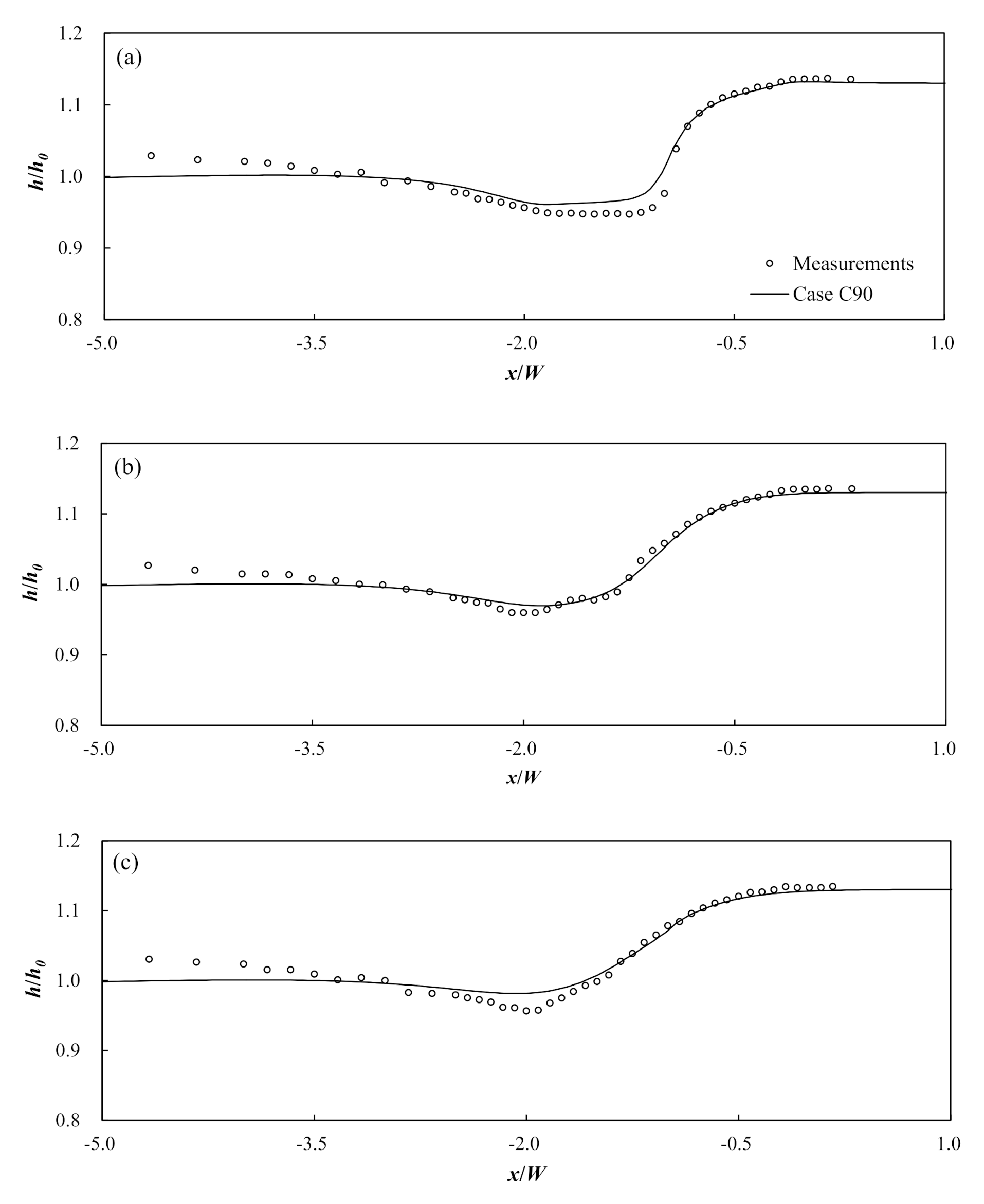
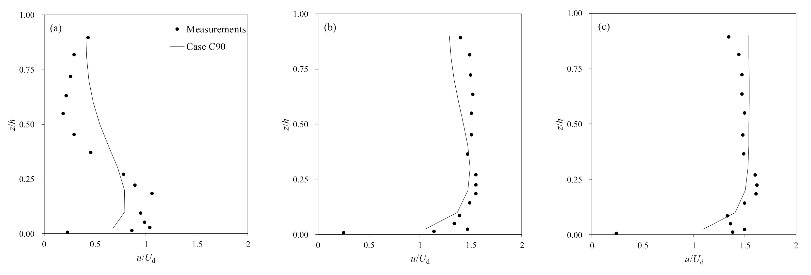
2.3. Model Settings and Validations

Numerical simulations were conducted to analyze changes in solute mixing with flow and mixing changes stemming from junction angle modifications. The channel used for numerical simulation was designed based on the laboratory experimental channel considered by Shumate [51], and the length scale was increased to 10 times the original size. Through simulations using the scaled-up channel, flow and mixing patterns in small-scale streams, which are often found in urban areas covered with concrete (n = 0.013) with a small width-to-depth ratio, were reproduced. According to the Froude similitude, the channel length, width, and discharge values used in our experiments are listed in

Table 2. Simulation conditions for flow and solute mixing analysis in channel confluence.

Case	α (°)	${\mathit{Q}}_{\mathit{m}}$ (m3/s)	${\mathit{Q}}_{\mathit{b}}$ (m3/s)	$\mathit{W}$ (m)	${\mathit{h}}_0$ (m)	${\mathit{C}}_0$ (ppm)	dt (s)	n, Manning’s Roughness Coefficient	${\mathit{M}}_{\mathit{r}}$	${\mathbf{Fr}}_{\mathit{d}}$
C90	90	13.6	40.2	9.14	2.96	100	0.005	0.013	1.62	0.37
C75	75
C60	60
C45	45
C30	30

. The confluence channel used for simulation was set to have the same width of $W=9.14 \mathrm{m}$ for the main and tributary channels in all cases. The downstream boundary water depth ($h_0$) for the numerical simulations was 2.96 m, which conforms to the geometric ratio. The junction angle was changed in 15° intervals with five cases, from 30° to 90°. Based on the results of grid sensitivity analysis, the grid size was set to be $W/dx>20$, and the number of vertical layers was set to 10 for the flow and mixing simulations by applying quasi-three-dimensional characteristics. The computational grids are presented in Figure 3.

For our simulations, the Smagorinsky model was adopted for RANS simulations, and the Smagorinsky constant varied from 0.15 to 0.40 to calculate the horizontal eddy viscosity and diffusion coefficient. The background vertical eddy viscosity was set to 2.09 $\times$ 10⁻² m²/s according to the depth-averaged value of parabolic distribution, where ${\epsilon }_z=\frac{1}{6}\kappa h{u}^{*}$, $\kappa =0.41$ is the von Karman constant, $u^{*}=\sqrt{g{R}_h{S}_f}$ is the shear velocity, $R_h$ is the hydraulic radius, and $S_f={\left(nU/R_h^{2/3}\right)}^2$. Time step (dt) was set to 0.005 s to satisfy the Courant–Friedrichs–Lewy (CFL) condition. The upstream boundary conditions for the main channel and tributary were set to a constant discharge, and the downstream boundary condition was set to a constant water depth, as listed in Table 2. The discharge of the main and tributary channels was set to ${\mathrm{Fr}}_d=0.37$ for a discharge ratio ($Q_r$) of 0.25, such that the numerical simulations would have a separation zone downstream of the junction. Based on these hydraulic conditions, the momentum flux ratio ($M_r$) in this study was 1.62, which is included in the range for previous studies (0.29–2.52) [16,30]. The free-slip condition was employed for the wall boundary. The kinematic boundary condition was applied for the free surface and bottom boundary, and w becomes 0 at the bottom and water surface. The EFDC model specifies the shear stress at the bottom cell layer for computation of the internal mode as

$$\left({\tau }_x^b, {\tau }_y^b\right)=c_b\sqrt{u_b^2+v_b^2}\left(u_b, v_b\right)$$

(15)

where ${\tau }_x^b$ and ${\tau }_y^b$ are the bottom shear stress; $u_b$ and $v_b$ are the horizontal velocity component at the bottom cell layer; $c_b={\kappa }^2/{\left[\ln \left(\Delta z/2z_0^{*}\right)\right]}^2$ is the bottom stress coefficient given assuming a logarithmic velocity profile where $\Delta z$ is the bottom cell layer thickness, and $z_0^{*}$ is the dimensional bottom roughness height [45]. In this study, $z_0^{*}$ was set to 1 mm. For the solute mixing simulations, a scenario with an accidental spill was considered for the analysis of solute storage effects in the recirculation zone. Therefore, a fully mixed neutrally buoyant solute was introduced for 5 s at a concentration of 100 ppm from the tributary channel. The no-flux boundary condition was applied to all boundaries for the solute mixing simulations.

To verify the accuracy of our simulations using grids following the Froude similitude, the experimental results from Shumate [51] were used for performing water depth and vertical velocity profile comparisons to the simulations, as shown in Figure 4 and Figure 5, respectively. A comparison with the experimental data and simulation data for the water depth for the Case C90 at the points of y/W = 0.17, 0.50, and 0.82 revealed an MAPE of 2.7% to 3.3%. The vertical variations of velocity were properly reproduced compared to the measurements except for the result shown in Figure 5a. The discrepancy at x/W = −1.0, y/W = 0.17 was caused by the hydrostatic assumption, which is insufficient to present the vertical pressure gradient in highly distorted velocity gradient due to the flow separation. Despite the discrepancies, the numerical simulation of the channel with scale enlargement following the Froude similitude adequately reproduced the experimental results.

3. Results

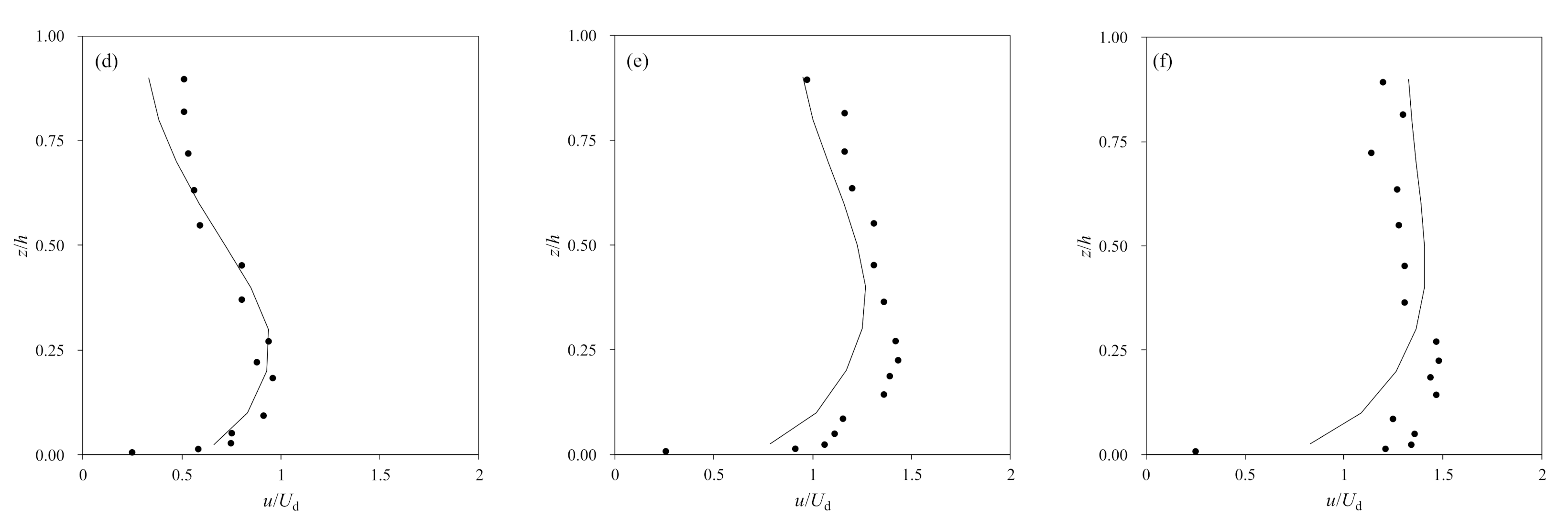
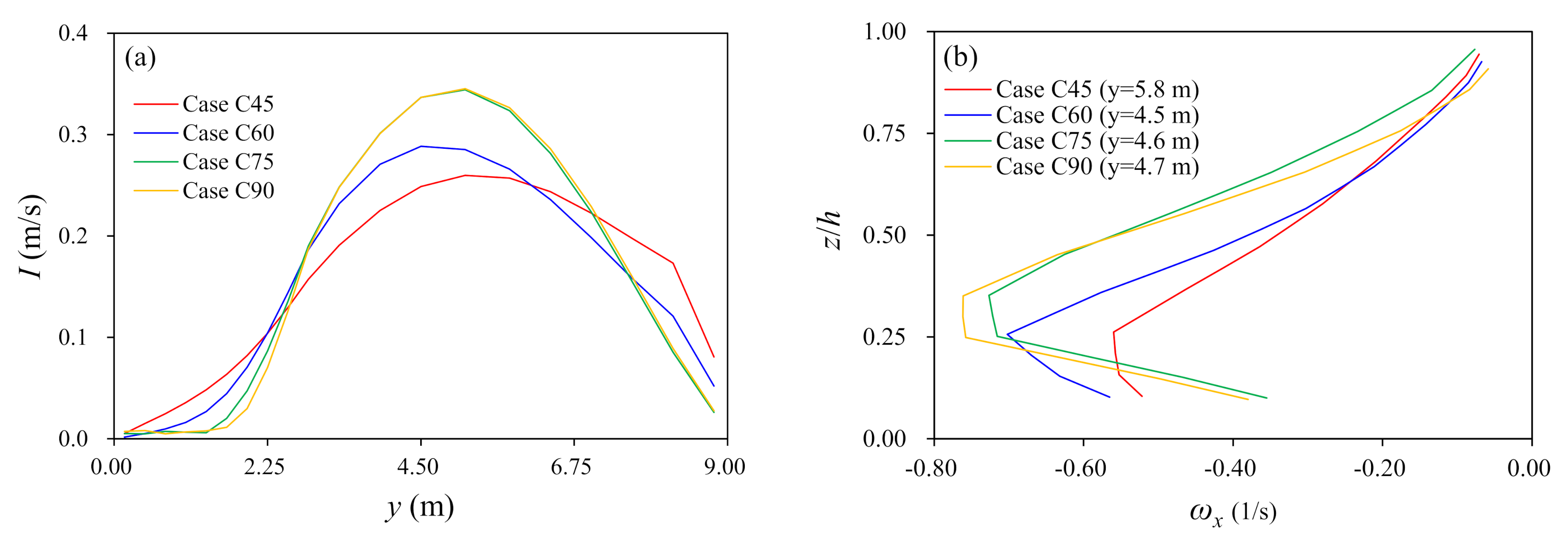
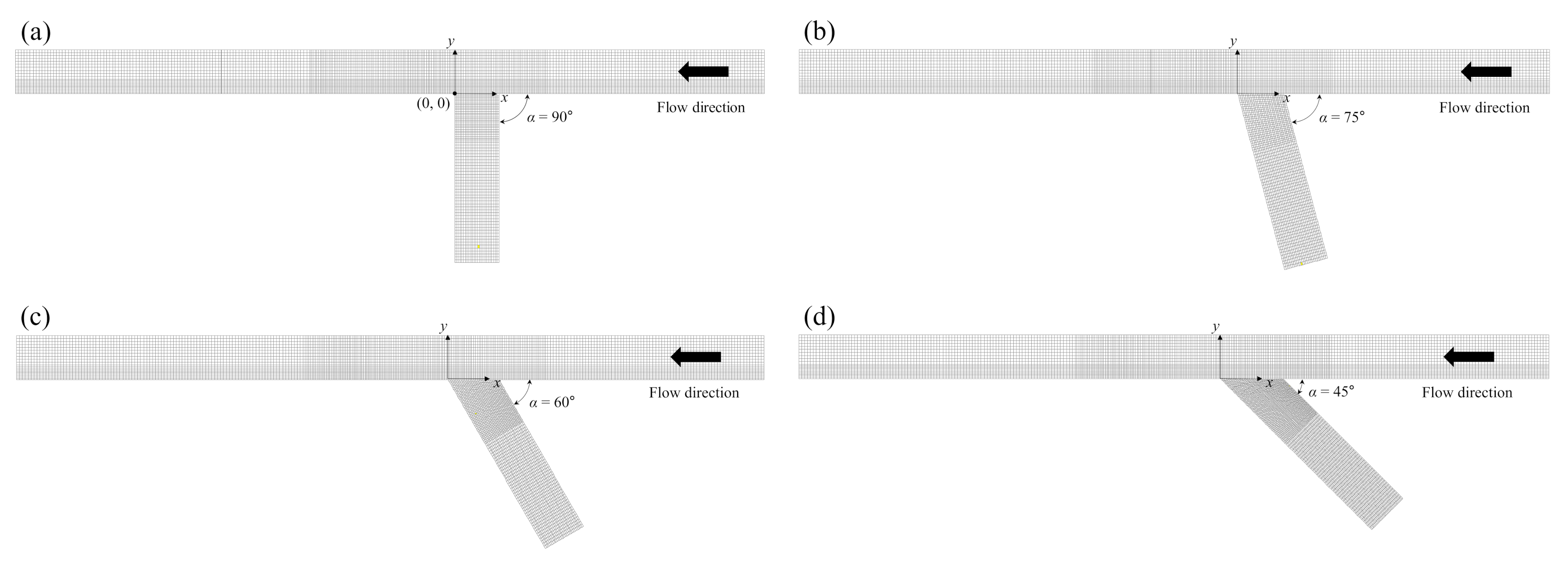
3.1. Effects of Junction Angle on Flow Characteristics

In this study, the reproducibility of the flow structures associated with the junction angle of the designed confluence was evaluated based on numerical simulation results. Figure 6 presents the depth-averaged velocity and streamlines in the recirculation zone developed by the tributary inflow. The inflow of the tributary causes flow separation and the maximum velocity is generated by flow contraction at the right bank. The stagnation zone appears in the upstream junction corner and the velocity at this point decreases. The size of the recirculation zone increases as the junction angle increases, which has been reported in previous studies [12,23,38,53].

Figure 7 compares the u and v–w velocity vectors at the cross-section in the middle of the recirculation zone depicted in Figure 6. The negative sign of the velocity contour in Figure 7 indicates flow heading in the downstream direction. The channel-scale helical cell is developed under the simulation conditions of $M_r>1$ [54]. As the junction angle increases, the center of the clockwise helical cell is positioned near the bottom of the channel. Figure 8 presents more detailed features of the transversal velocity associated with the clockwise helical motion shown in Figure 7. The depth-averaged vertical deviation of the v velocity is given as $I=\sqrt{{\displaystyle {\int }_0^h{v^{\prime }}^2}dz/h}$, where $v^{\prime }$ is the vertical deviation from the depth-averaged velocity ($\overline{v}$) and indicates the strength of the circular motion (Figure 8a). The maximum value of $I$ occurs in the C90 case and decreases as the junction angle decreases. At each of the maximum values of $I$, the vertical distributions of vorticity in the x-direction (ω_x) are plotted according to the junction angle (Figure 8b). The results also reveal that helical motion develops strongly as the junction angle increases. Additionally, the strength of the helical motion increases near the left bank (0 < y < 2 m), where the recirculation zone is developed as the junction angle decreases. This indicates that the transverse transport of the solute in the recirculation zone may be weakened as the junction angle increases.

In Figure 9, the length ($L_s/W$) and width ($b_s/W$) of the recirculation zone, based on the depth-averaged velocity fields shown in Figure 6, are compared to the results obtained using Equations (2) and (3), as suggested by Gurram et al. [38]. The values of $L_s/W$ and $b_s/W$ are significantly reduced in the range of 45°–75° in the simulation results. These $L_s/W$ changes are similar to those obtained using Equation (2), but in the C30 case, the recirculation zone length is overestimated in the simulation results. The results of $b_s/W$ exhibit some underestimation compared to the calculations using Equation (3). These discrepancies in the simulation results could have occurred as a result of the hydrostatic assumption in the EFDC model. However, despite these limitations of the model, the overall results of the numerical simulations only exhibit minor differences compared to the empirical equations based on experiments, and the trend of the recirculation zone area changes with changes in the junction angle was reproduced reasonably accurately.

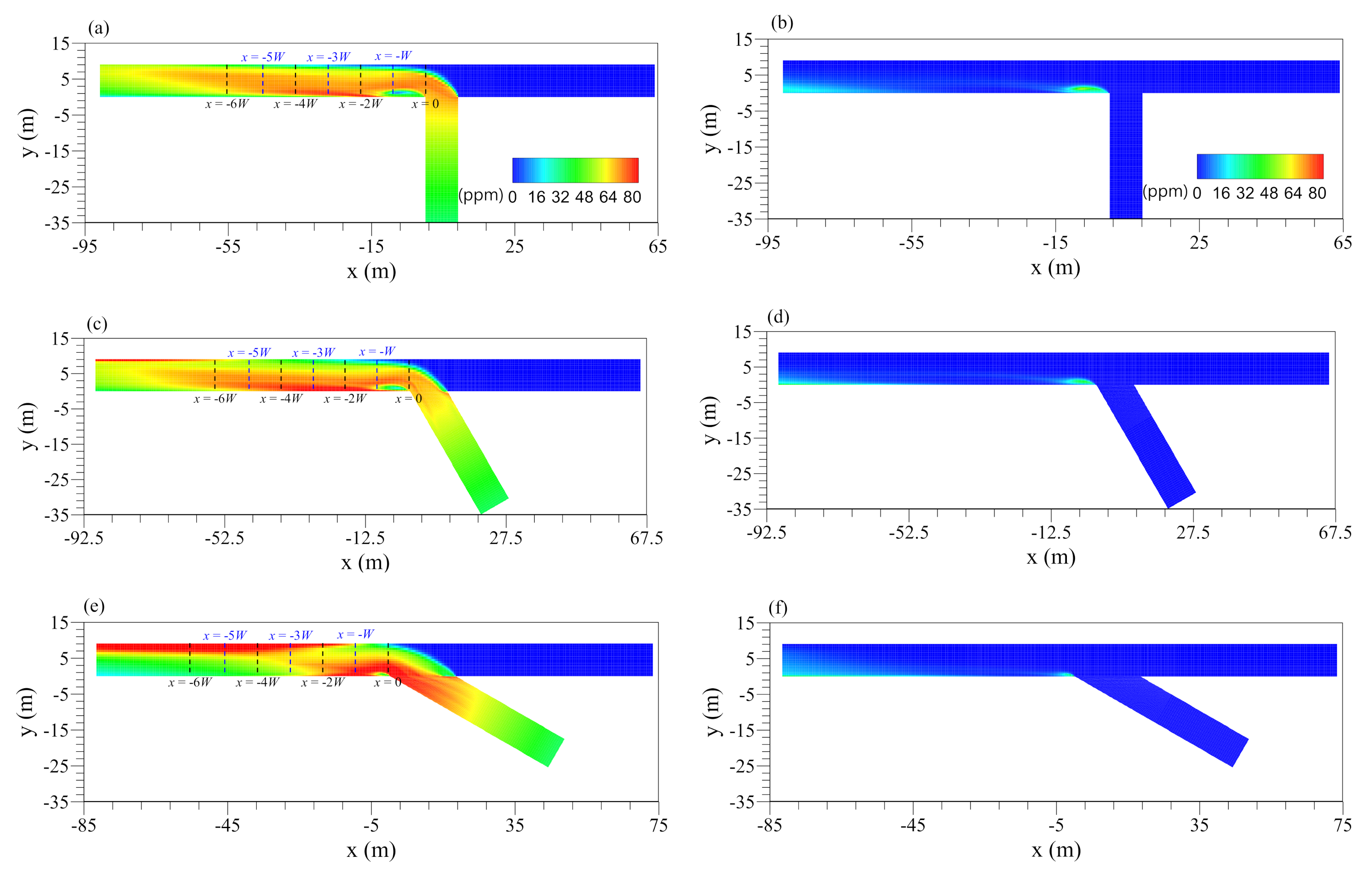
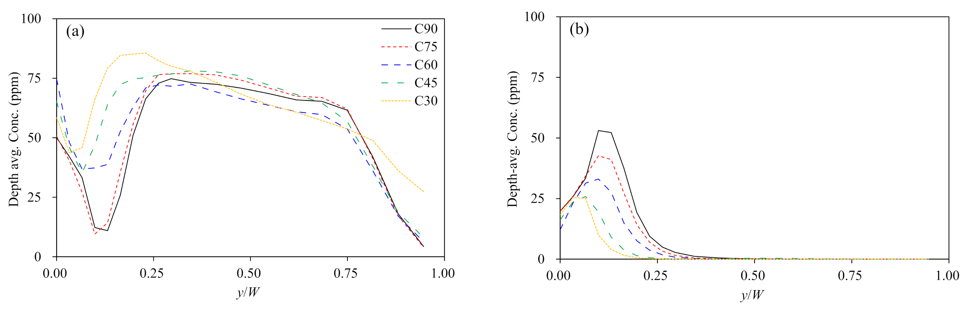
3.2. Solute Transport Results

The effect of junction angle on solute mixing was evaluated. Figure 10 presents the depth-averaged concentration distributions of the simulation results for t = 2.4 min and 4.1 min. When the solute cloud crosses the recirculation zone, a relatively small amount of solute inflows into the recirculation zone compared to the flow zone. The boundary layer created between the recirculation and flow zones disturbs solute trapping by the recirculation zone. Once the solute is trapped in the recirculation zone, it persists there for a relatively long time. Comparisons of the concentration in the recirculation zone revealed that the concentration in the C30 case was the highest after 2.4 min as a result of a relatively weakened boundary layer effect as the junction angle decreases. In contrast, after 4.1 min, the solute in the C90 case is retained the longest, resulting in a concentration that is higher than in the other simulation cases. The C30 case exhibits different mixing characteristics than the C60 and C90 cases because the solute input from the tributary bounces off the right bank, resulting in higher concentrations.

In Figure 11, the concentration distributions and streamlines of the v−w velocity, in the same cross-section shown in Figure 7, are depicted for t = 2.4 min. All cases reveal results in which the concentration at the bottom of the channel is relatively higher than that at the upper water surface. These results were obtained because the u velocity is lower at the bottom of the channel, resulting in less solute dispersion compared to the water surface, as shown in Figure 7. Additionally, the clockwise helical motion, which creates a strongly distorted mixing interface, causes rapid mixing with high discharge from the tributary. The distortion of the mixing interface results in an increase in the effects of $〈u^{\prime }{w}^{\prime }〉$ on turbulent diffusion [18]. As the junction angle increases, the vertical gradient of the mixing layer also increases as a result of the strongly developed helical cell. The solute cloud transported near the water surface by helical motion spreads to the outer bank. In contrast, near the channel bottom, the solute cloud moves to the inner bank where the recirculation zone is located. Then, the cloud is stored to accumulate the solute.

The transverse mixing of solute inflows from the tributary was analyzed using dosage curves, which were calculated using Equation (5). Figure 12 presents the transverse change in the dimensionless dosage ($\theta /\mathrm{\Theta }$) plotted versus the dimensionless cumulative discharge ($\eta$). The transverse distributions of $\theta /\mathrm{\Theta }$ gradually become flatter toward the downstream cross-section, except for the C30 case. In the C30 case in particular, $\theta /\mathrm{\Theta }$ increases at the right bank as a result of wall reflection. In the C45 case, wall reflection at the right bank causes an increase in $\theta /\mathrm{\Theta }$ from $x=-3W$. In the C75 and C90 cases, the effects of wall reflection rarely appear, even as far as $x=-5W$; in these cases, $\theta /\mathrm{\Theta }$ locally increases near the left bank at $x=-W$ and $x=-2W$ as a result of the recirculation zones. In the C90 case, the local increase in $\theta /\mathrm{\Theta }$ is maintained up to $x=-3W$.

The mixing metrics defined in Equation (4) can be utilized to evaluate transverse mixing. Figure 13 presents the changes in the dimensionless mixing metric (${\sigma }_r$), which was normalized using the standard deviation of the dosage curve at $x=0$ (${\sigma }_{us}$), as shown in Figure 12a. Upstream of $x=-2W$, the value of ${\sigma }_r$ was not affected by the junction angle, except for the C30 case. The C30 case shows that the deviation of the transverse dosage is minimized as a result of active transverse mixing, causing ${\sigma }_r$ to decrease quickly. However, as a result of wall reflection, ${\sigma }_r$ increases downstream of $x=-2W$, where transverse mixing is completed. These results indicate that as the junction angle decreases, transverse mixing becomes more active, causing a decrease in the transverse concentration deviation. In cases where the junction angle is below 45°, the tributary flow with high momentum causes the solute cloud to be transported to the far bank. Then, the solute is positioned near the outer bank as a result of wall reflection, resulting in an increase in the transverse concentration deviation.

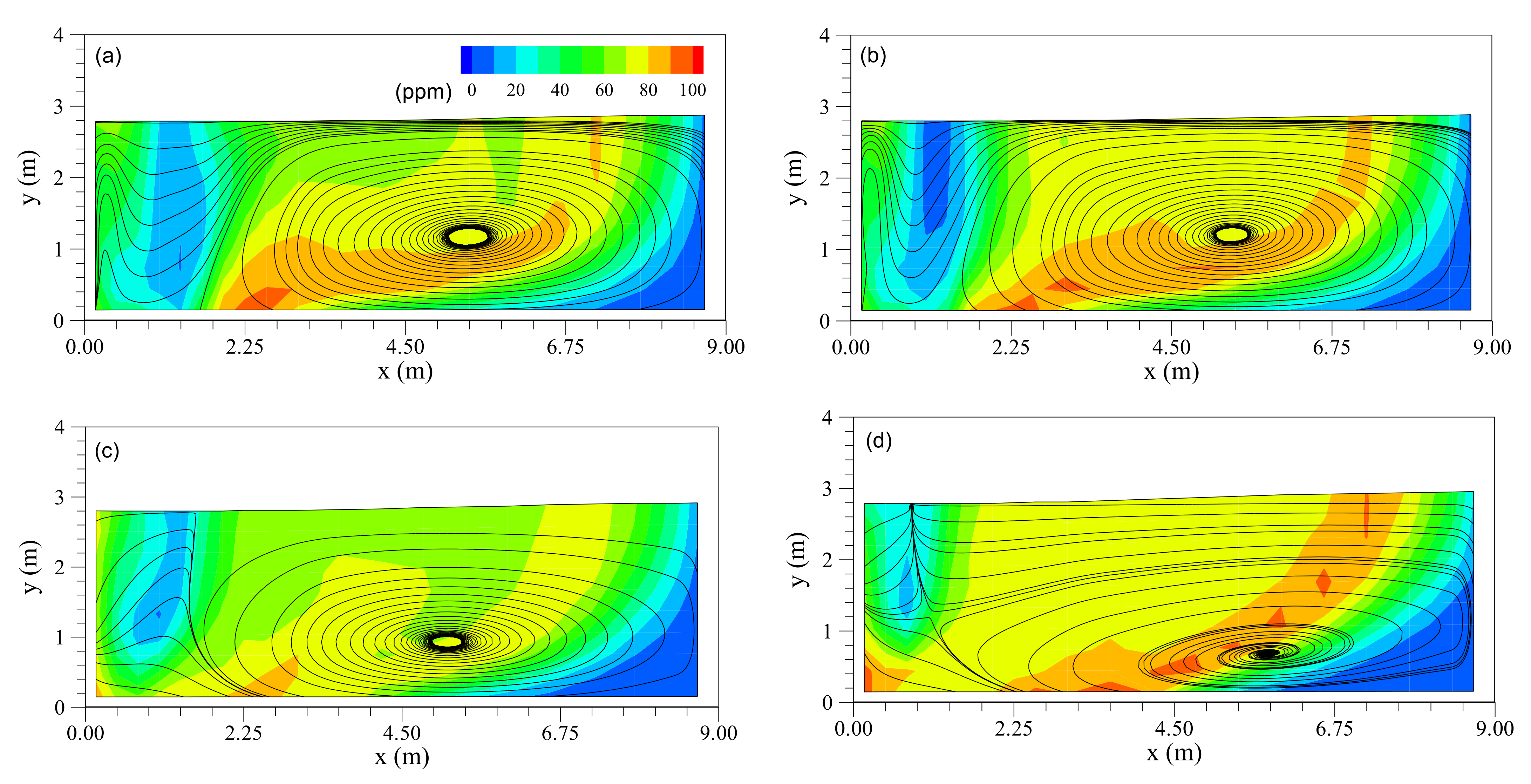
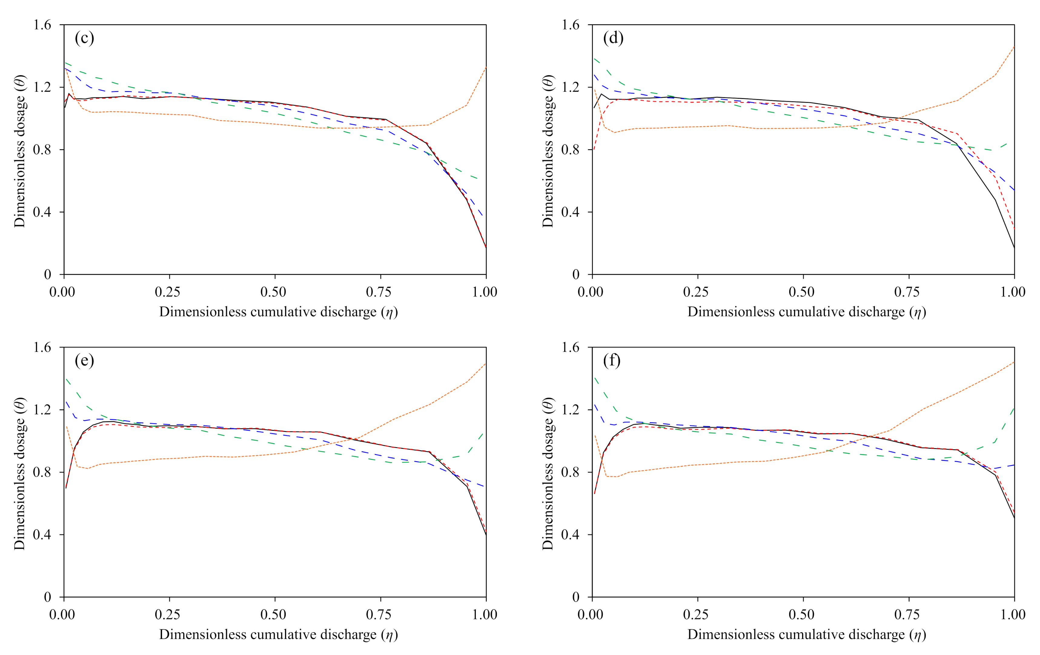
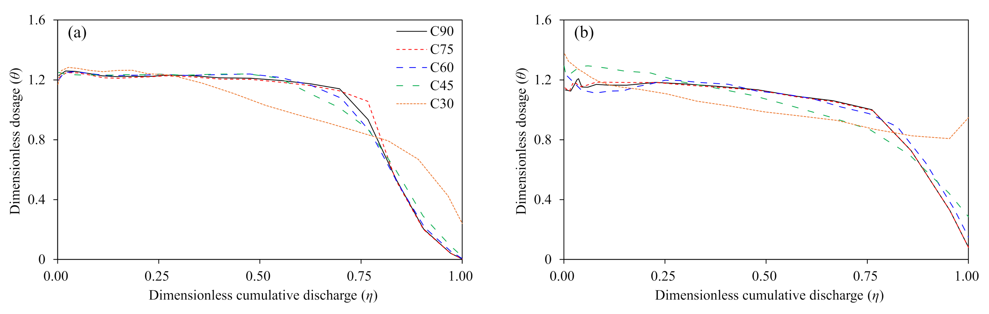
3.3. Storage Effects in the Recirculation Zone

To analyze the mixing properties in the recirculation zone, the concentration–time curves and skewness coefficient in the center of the recirculation zone are plotted in Figure 14. In Figure 14a, the rising limb of the concentration curve increases steeply while the falling limb decreases gradually, which is a typical property of mixing in the storage zones [55]. The strongly developed recirculation zone, which depends on an increase in the junction angle, leads to an increase in the maximum concentration in the storage zone. However, in the C30 case, the maximum concentration is higher than those in the C45 and C60 cases because the recirculation zone area is smaller than in those cases, allowing the passage of a relatively large amount of solute, as shown in Figure 10e. Figure 14b presents the results for the skewness coefficient of the concentration–time curves in Figure 14a. One can see that the skewness coefficient increases significantly as the junction angle increases, especially between 30° and 60°. These results demonstrate that the increase in the tail caused by solute trapping is stabilized at junction angles above 60°.

Figure 15 presents the transverse changes in concentration in cross-sections containing the center of the recirculation zone at t = 2.4 min and t = 4.1 min. At t = 2.4 min, the results reveal that a concentration dip occurs in the recirculation zone, and the lowest concentration tends to increase as the junction angle decreases. In contrast, at t = 4.1 min, the C90 case yields the highest concentration. Additionally, the maximum concentration decreases as the junction angle decreases. These results indicate that the concentration accumulated in the storage zone increases with the junction angle and that the retention time of the solute also increases.

4. Discussion

4.1. Solute Mixing Downstream of Junction

In this study, the effects of the junction angle on the mixing characteristics at the channel confluence and retention of the solute cloud in the storage zone were analyzed. First, the reproducibility of the flow pattern at the confluence was evaluated by changing the junction angle. Following the experimental research by Gurram et al. [38], the simulation results in this study also demonstrated that as the junction angle increases, the length and width of the recirculation zone increase. Additionally, the simulation results reproduced a clockwise helical cell, which was developed at the outer bank downstream of the confluence. Field measurements by Rhoads and Kenworthy [54] revealed similar results, where one secondary cell developed downstream of the junction under the condition of $M_r>1$. As the junction angle decreased, the center of the helical cell moved slowly toward the bottom of the channel (Figure 8) and showed similar results to Shakibainia et al. [23], where numerical simulations revealed a decrease in the u velocity. These previous studies verify the applicability and validity of the simulation results derived in this study.

Previous studies have reported that transverse mixing is related to the momentum flux ratio ($M_r$). Lewis et al. [16] and Lewis and Rhoads [41] reported that transverse mixing increases with $M_r$. Additionally, the results presented by Pouchoulin et al. [30] support the positive correlation between transverse mixing and $M_r$ based on field measurements, where $D_T/h{u}^{*}$ was 1.34, $M_r=1.15$ and 2.21, and $M_r=1.54$. However, analysis of the transverse dispersion associated with flow structures by junction angle has been limited in previous studies. In this research, simulation results demonstrated that transverse mixing depends on two main features: helical motion and recirculating flow. Therefore, the relationship between the two main flow features caused by the junction angle and transverse dispersion coefficients is presented in Figure 16. In Figure 16, $D_T/h{u}^{*}$ is calculated using Equation (8), resulting in a range of 0.32–0.82. These results show that $D_T/h{u}^{*}$ increases with the relative intensity of helical motion versus the u velocity $\frac{1}{W}{\displaystyle {\int }_0^{W}I} dy/\overline{u}$, where $\overline{u}$ is the depth-averaged u velocity (Figure 16a). In contrast, $D_T/h{u}^{*}$ decreases with an increase in the length (Figure 16b) and width of the recirculation zone (Figure 16c). Since the recirculation zone size changes over flow depth, these results are valid for the recirculation zone size based on the depth-averaged flow field. As the junction angle increases, the helical motion intensity decreases because the increase in the u velocity was more dominant than that in the v velocity as a result of flow contraction caused by the occurrence of a recirculation zone. Therefore, one can see that the interrelationship between the helical motion and recirculation zone caused by a change in the junction angle affects transverse mixing.

4.2. Storage Zone Effects on Transverse Mixing

The recirculation zone at a confluence traps the solute cloud and extends the retention time of the solute, as shown in Figure 10. However, the parameters that represent the storage zone characteristics are difficult to obtain from field measurements. In this study, the parameters for the storage zone model were estimated based on simulation results, and the relationships with transverse mixing in confluences were analyzed.

The main parameters for the storage zone model are the residence time ($T$), area of the developed recirculation zone ($A_s$), and relative percentage of the zone area among the total area ($\epsilon$).

Table 3. Storage zone model parameters for recirculation zones in confluences for different junction angles.

$\alpha$ (°)	90	75	60	45	30
$T$ (s)	77.52	76.34	73.53	71.94	50.76
$A_s$ (m2)	29.76	26.04	16.56	6.72	3.60
$\epsilon$	0.24	0.22	0.18	0.14	0.11
$\epsilon /T$ (s−1)	3.10 $\times$ 10−3	2.88 $\times$ 10−3	2.45 $\times$ 10−3	1.95 $\times$ 10−3	2.17 $\times$ 10−3

lists the estimated storage zone model parameters, which were obtained from the recirculation zone in the depth-averaged flow field. $T$ was calculated using Equation (13) based on the averaged concentration-time curves in the recirculation zone. $A_s$ was determined as the area of the recirculation zone, and $\epsilon$ was calculated from the area of the horizontal plane containing the recirculation zone. These results indicate that all storage zone parameters decrease as the junction angle decreases as a result of a weakened recirculation zone, as shown in Figure 6. When the junction angle decreases from 90° to 45°, $T$ gradually decreases, but the decrease is substantial at 30°. These results indicate that the solute storage effect of the recirculation zone is greatly reduced when the relative area of the storage zone ($\epsilon$) reaches approximately 11%.

In natural streams containing storage zones, 1D longitudinal mixing is achieved by shear flow dispersion and mixing in the storage zone, as shown in Equation (10). Regarding the relationship between shear flow dispersion and storage zone effects, Choi et al. [56] demonstrated a negative correlation between the mass exchange rate ($\epsilon /T$) and longitudinal dispersion coefficient in the flow zone ($K_f$). This inverse relationship can be said to reduce the shear flow dispersion, as mixing by the storage zone is strengthened. Additionally, this study revealed that the existence of a recirculation zone affects transverse mixing. Therefore, to discuss the storage effects on transverse mixing due to a recirculation zone, the relationship between $\epsilon /T$ and $D_T/h{u}^{*}$ is plotted in Figure 17. Similar to the relationship between $\epsilon /T$ and $K_f$, $D_T/h{u}^{*}$ also has a negative correlation with $\epsilon /T$. As in Fischer et al. [40], the longitudinal shear dispersion has an inverse relationship with the transverse dispersion coefficient; in the present study, the decrease in $D_T/h{u}^{*}$ leads to an increase in longitudinal shear dispersion. Therefore, $\epsilon /T$ and $D_T/h{u}^{*}$ simultaneously reduce the longitudinal shear dispersion, and transverse mixing is replaced by mixing in the storage zone when the recirculation zone is strongly developed.

5. Conclusions

The paper presents the results of a numerical study about the effect of junction angle on flow structure and transverse mixing at a confluence. Flow and mixing analyses in confluences were conducted under conditions of $M_r=1.62$ and $\alpha ={30}^{\circ }-{90}^{\circ }$ to analyze the storage effects caused by recirculation zones. In this study, the following results were obtained:

• As the junction angle increases, the strength of helical motion and vorticity magnitude increase, leading to an increase in the vertical gradient of the mixing layer and mixing metric of the dosage curves.
• The recirculation zone creates a boundary layer that interrupts the inflow of solute and simultaneously accumulates solute. These storage effects of the recirculation zone generate long-tailed concentration curves, where the skewness significantly increases at junction angles of 30° to 60°.
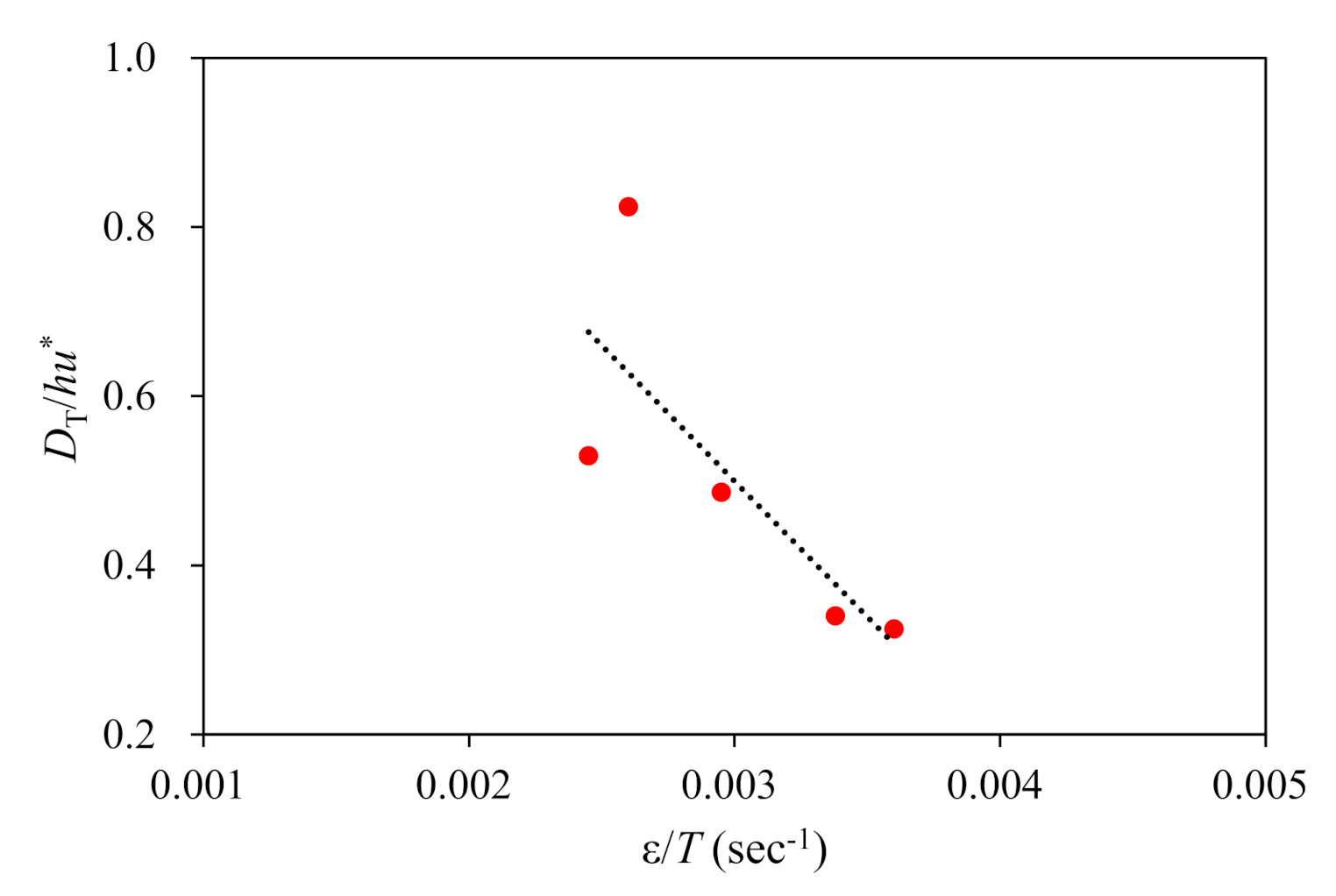
• The interaction between the helical motion and recirculation zone affects transverse mixing, where the transverse dispersion coefficient exhibits a positive correlation with the helical motion intensity and negative correlation with the recirculation zone size.
• The transverse dispersion coefficient has an inverse relationship with the mass exchange rate of the storage zone. Based on these results, it can be inferred that transverse dispersion is replaced by mixing due to strongly developed storage zones.

The aforementioned analysis results are limited to the case of $M_r=1.62$ and to the time-averaged flow field. Despite the properly reproduced flow simulation results, the solute mixing simulation results have limitations because the results were not completely validated using experimental results. Therefore, additional detailed research on solute and solids mixing due to the storage zone would require a mass exchange rate based on turbulence structures near recirculation zone boundaries.

References

1. Taylor, G.I. The dispersion of matter in turbulent flow through a pipe. Proc. R. Soc. Lond. Math. Phys. Eng. Sci. 1954, 223, 446–468. [Google Scholar]
2. Rana, S.M.M.; Scott, D.T.; Hester, E.T. Effects of in-stream structures and channel flow rate variation on transient storage. J. Hydrol. 2017, 548, 157–169. [Google Scholar] [CrossRef] [Green Version]
3. Jackson, T.R.; Haggerty, R.; Apte, S.V. A fluid-mechanics based classification scheme for surface transient storage in riverine environments: Quantitatively separating surface from hyporheic transient storage. Hydrol. Earth Syst. Sci. 2013, 17, 2747–2779. [Google Scholar] [CrossRef] [Green Version]
4. Bencala, K.E.; Walters, R.A. Simulation of solute transport in a mountain pool-and riffle stream: A transient storage model. Water Resour. Res. 1983, 19, 718–724. [Google Scholar] [CrossRef]
5. Runkel, R.L. One-Dimensional Transport with Inflow and Storage (OTIS): A Solute Transport Model for Streams and Rivers; US Department of the Interior, US Geological Survey: Washington, DC, USA, 1998; Volume 98.
6. Seo, I.W.; Cheong, T.S. Moment-Based calculation of parameters for the storage zone model for river dispersion. J. Hydraul. Eng. 2001, 127, 453–465. [Google Scholar] [CrossRef]
7. Kelleher, C.; Wagener, T.; McGlynn, B.; Ward, A.S.; Gooseff, M.N.; Payn, R.A. Identifiability of transient storage model parameters along a mountain stream. Water Resour. Res. 2013, 49, 5290–5306. [Google Scholar] [CrossRef]
8. Rodrigues, P.P.G.W.; Gonzalez, Y.M.; de Sousa, E.P.; Neto, F.D.M. Evaluation of dispersion parameters for River Sao Pedro, Brazil, by the simulated annealing method. Inverse Probl. Sci. Eng. 2013, 21, 34–51. [Google Scholar] [CrossRef]
9. Femeena, P.V.; Chaubey, I.; Aubeneau, A.; McMillan, S.; Wagner, P.D.; Fohrer, N. Simple regression models can act as calibration-substitute to approximate transient storage parameters in streams. Adv. Water Resour. 2019, 123, 201–209. [Google Scholar] [CrossRef]
10. Noh, H.; Kwon, S.; Seo, I.W.; Baek, D.; Jung, S.H. Multi-gene genetic programming regression model for prediction of transient storage model parameters in natural rivers. Water 2021, 13, 76. [Google Scholar] [CrossRef]
11. Jung, S.H.; Seo, I.W.; Kim, Y.D.; Park, I. Feasibility of velocity-based method for transverse mixing coefficients in river mixing analysis. J. Hydraul. Eng. 2019, 145, 04019040. [Google Scholar] [CrossRef]
12. Best, J.L.; Reid, I. Separation zone at open-channel junctions. J. Hydraul. Eng. 1984, 110, 1588–1594. [Google Scholar] [CrossRef]
13. Rhoads, B.L.; Riley, J.D.; Mayer, D.R. Response of bed morphology and bed material texture to hydrological conditions at an asymmetrical stream confluence. Geomorphology 2009, 190, 161–173. [Google Scholar] [CrossRef]
14. Ramón, C.L.; Hoyer, A.B.; Armengol, J.; Dolz, J.; Rueda, F.J. Mixing and circulation at the confluence of two rivers entering a meandering reservoir. Water Resour. Res. 2013, 49, 1429–1445. [Google Scholar] [CrossRef]
15. Horna-Munoz, D.; Constantinescu, G.; Rhoads, B.; Lewis, Q.; Sukhodolov, A. Density effects at a concordant bed natural river confluence. Water Resour. Res. 2020, 58, e2019WR026217. [Google Scholar] [CrossRef]
16. Lewis, Q.; Rhoads, B.; Sukhodolov, A.; Constantinescu, G. Advective lateral transport of streamwise momentum governs mixing at small river confluence. Water Resour. Res. 2020, 56, e2019WR026817. [Google Scholar] [CrossRef]
17. Schindfessel, L.; Creelle, S.; Mulder, T.D. Flow patterns in an open channel confluence with increasingly dominant tributary inflow. Water 2015, 7, 4724–4751. [Google Scholar] [CrossRef] [Green Version]
18. Yuan, S.; Tang, H.; Xiao, Y.; Qiu, X.; Zhang, H.; Yu, D. Turbulent flow structure at a 90-degree open channel confluence: Accounting for the distortion of the shear layer. J. Hydro-Environ. Res. 2016, 12, 130–147. [Google Scholar] [CrossRef] [Green Version]
19. Gualtieri, C.; Filizola, N.; de Oliveira, M.; Santos, A.M.; Ianniruberto, M. A field study of the confluence between Negro and Solimões Rivers. Part 1: Hydrodynamics and sediment transport. C. R. Geosci. 2018, 350, 31–42. [Google Scholar] [CrossRef]
20. Yuan, S.; Tang, H.; Li, K.; Xu, L.; Xiao, Y.; Gualtieri, C.; Rennie, C.; Melville, B. Hydrodynamics, sediment transport and morphological features at the confluence between the Yangtze River and the Poyang Lake. Water Resour. Res. 2020, 57, e2020WR028284. [Google Scholar] [CrossRef]
21. Huang, J.; Weber, L.J.; Lai, Y.G. Three-dimensional numerical study of flows in open-channel junctions. J. Hydraul. Eng. 2002, 128, 268–280. [Google Scholar] [CrossRef]
22. Biron, P.M.; Ramamurthy, A.S.; Han, S. Three-dimensional numerical modeling of mixing at river confluences. J. Hydraul. Eng. 2004, 130, 243–253. [Google Scholar] [CrossRef]
23. Shakibainia, A.; Tabatabai, M.R.M.; Zarrati, A.R. Three-dimensional numerical study of flow structure in channel confluences. Can. J. Civ. Eng. 2010, 37, 772–781. [Google Scholar] [CrossRef]
24. Rooniyan, F. The effect of confluence angle on the flow pattern at a rectangular open-channel. Eng. Technol. Appl. Sci. Res. 2014, 4, 576–580. [Google Scholar] [CrossRef]
25. Lyubimova, T.P.; Lepikhin, A.P.; Parshakova, Y.N.; Kolchanov, V.Y.; Gualtieri, C.; Roux, B.; Lane, S.N. A numerical study of the influence of channel-scale secondary circulation on mixing processes downstream of river junctions. Water 2020, 12, 2969. [Google Scholar] [CrossRef]
26. Constantinescu, G.S.; Miyawaki, S.; Rhoads, B.; Sukhodolov, A.; Kirkil, G. Structure of turbulent flow at a river confluence with momentum and velocity ratio close to 1: Insights from an eddy-resolving numerical simulation. Water Resour. Res. 2011, 47, W05507. [Google Scholar] [CrossRef]
27. Constantinescu, G.; Miyawaki, S.; Rhoads, B.; Sukhodolov, A. Numerical analysis of the effect of momentum ratio on the dynamics and sediment-entrainment capacity of coherent flow structures at a stream confluence. J. Geophys. Res. 2012, 117, 1–21. [Google Scholar] [CrossRef]
28. Constantinescu, G.; Miyawaki, S.; Rhoads, B.; Sukhololov, A. Influence of planform geometry and momentum ratio on thermal mixing at a stream confluence with a concordant bed. Environ. Fluid Mech. 2016, 16, 845–873. [Google Scholar] [CrossRef]
29. Cheng, Z.; Constantinescu, G. Shallow mixing layers between non-parallel streams in a flat-bed wide channel. J. Fluid Mech. 2021, 916, 1–37. [Google Scholar] [CrossRef]
30. Pouchoulin, S.; Coz, J.L.; Mignot, E.; Gond, L.; Riviere, N. Predicting transverse mixing efficiency downstream of a river confluence. Water Resour. Res. 2019, 56, e2019WR026367. [Google Scholar] [CrossRef]
31. Lane, S.N.; Parsons, D.R.; Best, J.L.; Orfeo, O.; Kostaschuk, R.A.; Hardy, R.J. Causes of rapid mixing at a junction of two large rivers: Rio Parana and Rio Paraguay, Argentina. J. Geophys. Res. Earth Surf. 2008, 113, 1–16. [Google Scholar] [CrossRef] [Green Version]
32. Ramón, C.L.; Armengol, J.; Dolz, J.; Prats, J.; Rueda, F.J. Mixing dynamics at the confluence of two large rivers undergoing weak density variations. J. Geophys. Res. Oceans 2014, 119, 2386–2402. [Google Scholar] [CrossRef]
33. Gualtieri, C.; Ianniruberto, M.; Filizola, N. On the mixing of rivers with a difference in density: The study case of the Negro/Solimões confluence, Brazil. J. Hydrol. 2019, 578, 124029. [Google Scholar] [CrossRef]
34. Kim, K.; Park, M.; Min, J.H.; Ryu, I.; Kang, M.R.; Park, L.J. Simulation of algal bloom dynamics in a river with the ensemble Kalman filter. J. Hydrol. 2014, 519, 2810–2821. [Google Scholar] [CrossRef]
35. Zhu, Z.; Oberg, N.; Morales, V.M.; Quijano, J.C.; Landry, B.J.; Garcia, M.H. Integrated urban hydrologic and hydraulic modelling in Chicago, Illinois. Environ. Model. Softw. 2016, 77, 63–70. [Google Scholar] [CrossRef]
36. Weiskerger, C.J.; Phanikumar, M.S. Numerical modeling of microbial fate and transport in natural waters: Review and implications for normal and extreme storm events. Water 2020, 12, 1876. [Google Scholar] [CrossRef]
37. Tinh, N.X.; Tanaka, H.; Abe, G.; Okamoto, Y.; Pakoksung, K. Mechanisms of flood-induced levee breaching in Marumori town during the 2019 Hagibis typhoon. Water 2021, 13, 244. [Google Scholar] [CrossRef]
38. Gurram, S.K.; Karki, K.S.; Hager, W.H. Subcritical junction flow. J. Hydraul. Eng. 1997, 123, 447–455. [Google Scholar] [CrossRef]
39. Gualtieri, C. RANS-based simulation of transverse turbulent mixing in a 2D geometry. Environ. Fluid Mech. 2010, 10, 137–156. [Google Scholar] [CrossRef]
40. Fischer, H.B.; List, J.E.; Koh, R.C.Y.; Imberger, J.; Brooks, N.H. Mixing in Inland and Coastal Waters, 2nd ed.; Academic Press: San Diego, CA, USA, 1979. [Google Scholar]
41. Lewis, Q.W.; Rhoads, B.L. Rates and patterns of thermal mixing at a small stream confluence under variable incoming flow conditions. Hydrol. Process. 2015, 29, 4442–4456. [Google Scholar] [CrossRef]
42. Beltaos, S. Evaluation of transverse mixing coefficients from slug tests. J. Hydraul. Res. 1975, 13, 351–360. [Google Scholar] [CrossRef]
43. Kim, J.S.; Baek, D.; Park, I. Evaluating the impact of turbulence closure models on solute transport simulations in meandering open channels. Appl. Sci. 2020, 10, 2769. [Google Scholar] [CrossRef]
44. Nordin, C.F.; Troutman, B.M. Longitudinal dispersion in rivers: The persistence of skewness in observed data. Water Resour. Res. 1980, 16, 123–128. [Google Scholar] [CrossRef]
45. Hamrick, J.M. A three-dimensional environmental fluid dynamics computer code: Theoretical and computational aspects. In Special Report in Applied Marine Science and Ocean Engineering, 317; Virginia Institute of Marine Science: Gloucester Point, VA, USA, 1992; pp. 7–9. [Google Scholar]
46. Smagorinsky, J. General circulation experiments with the primitive equations. Mon. Weather Rev. 1963, 91, 99–164. [Google Scholar] [CrossRef]
47. Mellor, G.L.; Yamada, T. Development of a turbulence closure model for geophysical fluid problems. Rev. Geophys. Space Phys. 1982, 20, 851–875. [Google Scholar] [CrossRef] [Green Version]
48. Constantinescu, G. Le of shallow mixing interfaces: A review. Environ. Fluid Mech. 2014, 14, 971–996. [Google Scholar] [CrossRef]
49. Cheng, Z.; Constantinescu, G. Stratification effects on flow hydrodynamics and mixing at a confluence with a highly discordant bed and a relatively low velocity ratio. Water Resour. Res. 2018, 54, 4537–4562. [Google Scholar] [CrossRef]
50. Gualtieri, C.; Angeloudis, A.; Bombardelli, F.; Jha, S.; Stosser, T. On the values for the turbulent Schmidt number in environmental flows. Fluids 2020, 2, 17. [Google Scholar] [CrossRef] [Green Version]
51. Shumate, E.D. Experimental Description of Flow at an Open-Channel Junction. Master’s Thesis, University of Iowa, Iowa City, IA, USA, 1 December 1998. [Google Scholar]
52. Song, C.G.; Seo, I.W.; Kim, Y.D. Analysis of secondary current effect in the modeling of shallow flow in open channels. Adv. Water Resour. 2012, 41, 29–48. [Google Scholar] [CrossRef]
53. Penna, N.; Marchis, M.D.; Canelas, O.B.; Napoli, E.; Cardoso, A.; Gaudio, R. Effect of the junction angle on turbulent flow at a hydraulic confluence. Water 2018, 10, 469. [Google Scholar] [CrossRef] [Green Version]
54. Rhoads, B.L.; Kenworthy, S.T. Flow structure at an asymmetrical stream confluence. Geomorphology 1995, 11, 273–293. [Google Scholar] [CrossRef]
55. Park, I.; Seo, I.W. Modeling non-Fickian pollutant mixing in open channel flows using two-dimensional particle dispersion model. Adv. Water Resour. 2018, 111, 105–120. [Google Scholar] [CrossRef]
56. Choi, S.Y.; Seo, I.W.; Kim, Y.O. Parameter uncertainty estimation of transient storage model using Bayesian inference with formal likelihood based on breakthrough curve segmentation. Environ. Model. Softw. 2020, 123, 104558. [Google Scholar] [CrossRef]
Figure 1. Conceptual diagram of flow and mixing characteristics near channel confluence.
Applsci 11 11607 g001
Figure 2. Grid sensitivity analysis results for a 90° confluence angle: (a) Mean percentage error for the recirculation zone; (b) Mean percentage error for the water depth.
Applsci 11 11607 g002
Figure 3. Computational grids in xy plane: (a) C90; (b) C75; (c) C60; (d) C45.
Applsci 11 11607 g003
Figure 4. Comparisons of water depth for Case C90: (a) y/W = 0.17; (b) y/W = 0.50; (c) y/W = 0.82.
Applsci 11 11607 g004
Figure 5. Comparisons of vertical profiles of velocity for Case C90: (a) x/W = −1.0, y/W = 0.17; (b) x/W = −1.0, y/W = 0.50; (c) x/W = −1.0, y/W = 0.82; (d) x/W = −2.5, y/W = 0.17; (e) x/W = −2.5, y/W = 0.50; (f) x/W = −2.5, y/W = 0.82. Ud is the downstream cross-sectional averaged velocity.
Applsci 11 11607 g005aApplsci 11 11607 g005b
Figure 6. Depth-averaged velocity contours and streamlines near the recirculation zone: (a) C90; (b) C75; (c) C60; (d) C45; (e) C30.
Applsci 11 11607 g006
Figure 7. Comparisons of u-velocity magnitude and vw velocity vectors at the center of the recirculation zone: (a) C90 (x* = 6.7 m); (b) C75 (x* = 6.6 m); (c) C60 (x* = 5.1 m); (d) C45 (x* = 2.7 m). Negative velocity indicates a flow direction heading downstream.
Applsci 11 11607 g007
Figure 8. Properties of clock-wise helical cell by junction angle: (a) Lateral variations of the depth-averaged transversal velocity deviations; (b) Vertical distributions of the x-directional vorticity at the center of clockwise helical cell.
Applsci 11 11607 g008
Figure 9. Recirculation zone size versus junction angle: (a) Recirculation zone length; (b) Recirculation zone width.
Applsci 11 11607 g009
Figure 10. Depth-averaged concentration field with C-y curves: (a) C90 (t = 2.4 min); (b) C90 (t = 4.1 min); (c) C60 (t = 2.4 min); (d) C60 (t = 4.1 min); (e) C30 (t = 2.4 min); (f) C30 (t = 4.1 min).
Applsci 11 11607 g010
Figure 11. Concentration contours with streamlines in the recirculation zone at t = 2.4 min: (a) C90 (x* = 6.7 m); (b) C75 (x* = 6.6 m); (c) C60 (x* = 5.1 m); (d) C45 (x* = 2.7 m).
Applsci 11 11607 g011
Figure 12. Dimensionless cumulative discharge versus dimensionless dosage at: (a) x = 0; (b) x = −W; (c) x = −2W; (d) x = −3W; (e) x = −4W; (f) x = −5W.
Applsci 11 11607 g012aApplsci 11 11607 g012b
Figure 13. Dimensionless mixing metric for the simulated cases.
Applsci 11 11607 g013
Figure 14. Properties of concentration–time curves in the recirculation zone according to the junction angle: (a) Concentration–time curves; (b) Skewness coefficient of the concentration–time curves.
Applsci 11 11607 g014
Figure 15. Lateral distribution of the depth-averaged concentration in the center of the recirculation zone for different simulated cases: (a) t = 2.4 min; (b) t = 4.1 min.
Applsci 11 11607 g015
Figure 16. Relationship between the transverse dispersion coefficient and flow characteristics in confluences: (a) Intensity of helical motion; (b) Change in length; (c) Change in width.
Applsci 11 11607 g016
Figure 17. Relationship between the transverse dispersion coefficient and mass exchange rate.
Applsci 11 11607 g017