
A New Empirical Approach for Estimating Solar Insolation Using Air Temperature in Tropical and Mountainous Environments


Abstract
:1. Introduction
1.1. Background
1.2. Contribution
1.3. Paper Structure
2. Materials and Methods
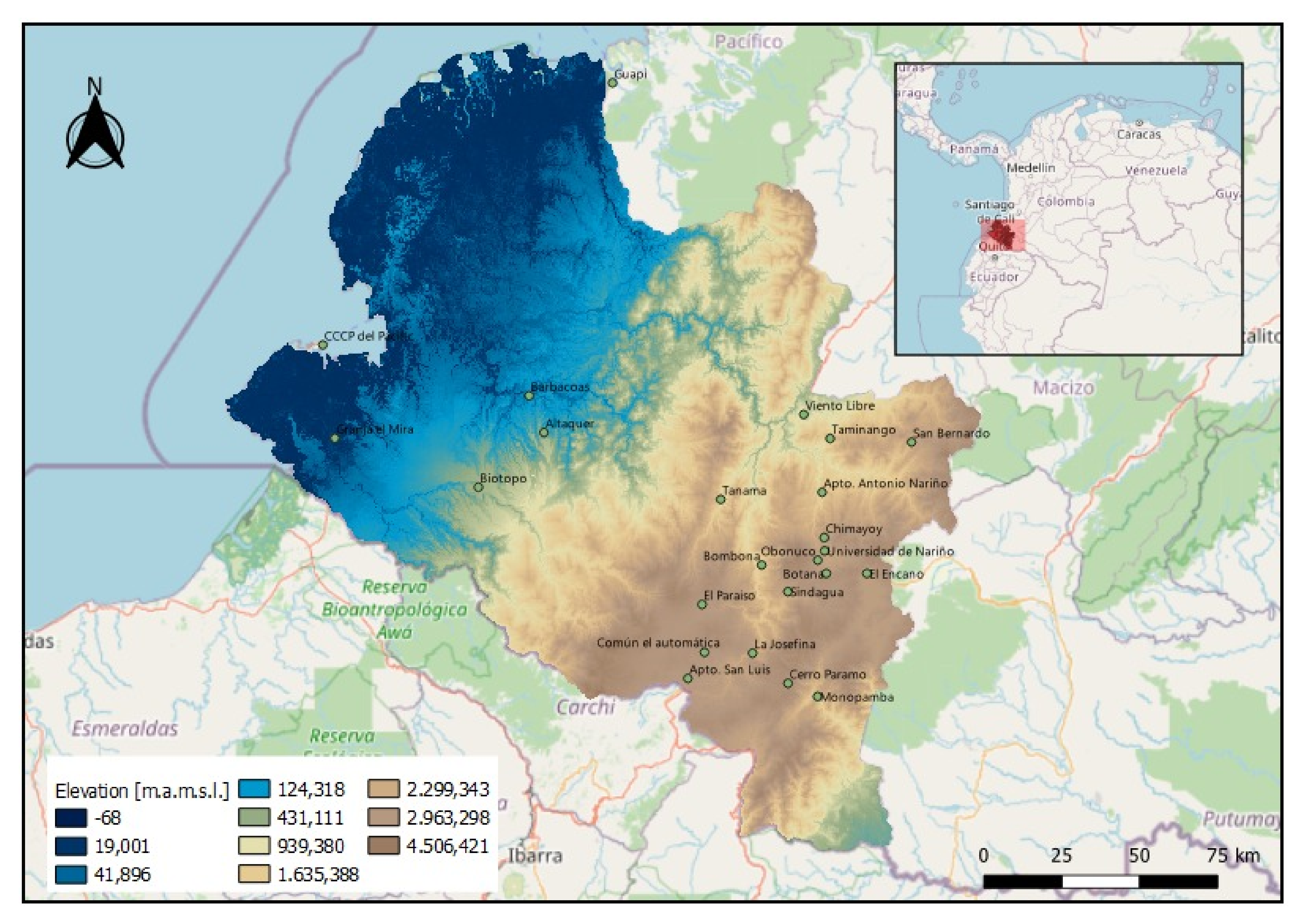
2.1. Site and Dataset
2.2. Data Quality Control
2.2.1. Solar Irradiance Data Quality Control
2.2.2. Temperature Data Quality Control
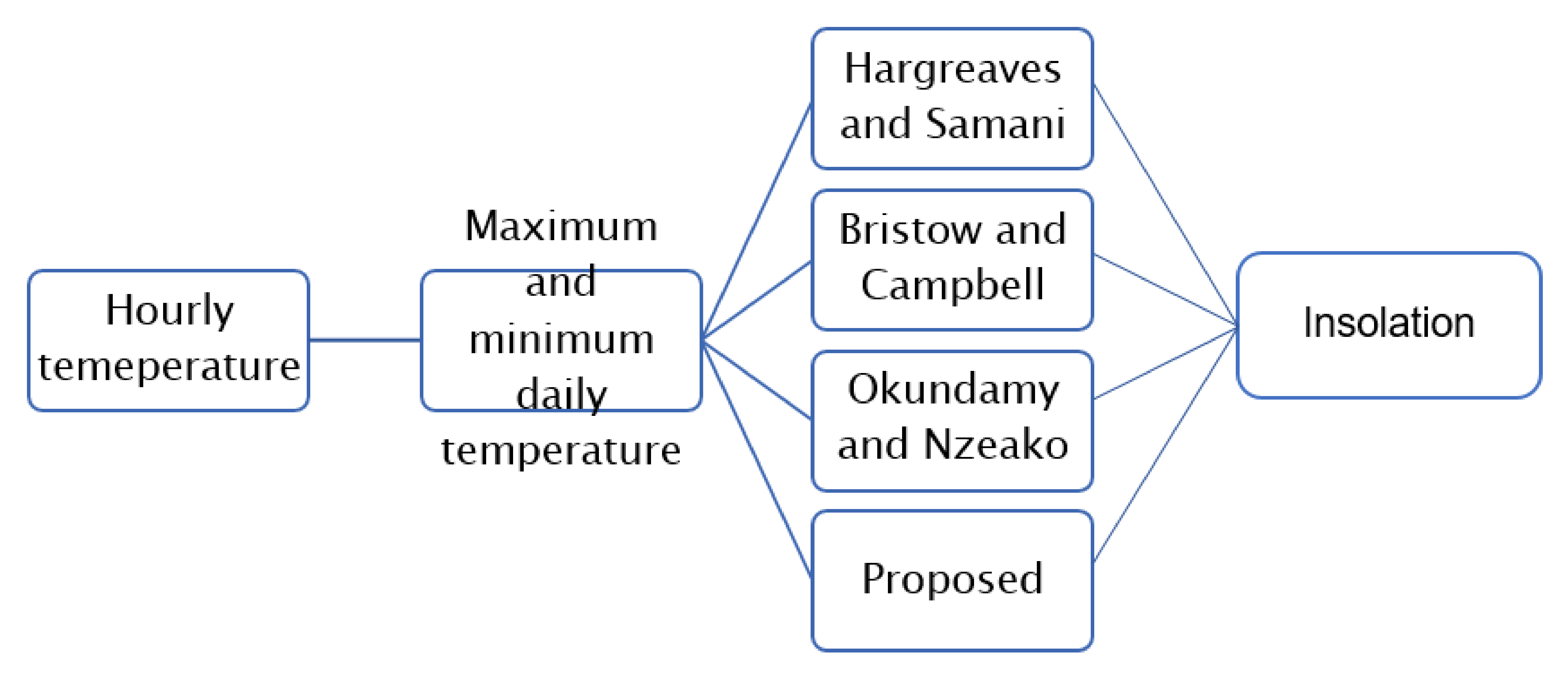
2.3. Empirical Temperature-Based Models
2.3.1. Hargreaves and Samani’s Model
2.3.2. Bristow and Campbell’s Model
2.3.3. Models Implemented in Tropical Environments
2.3.4. Proposed Empirical Model
2.4. Statistical Validation
3. Results and Discussion
3.1. Quality Control: Global Solar Irradiance and Temperature
3.2. Model Development and Performance
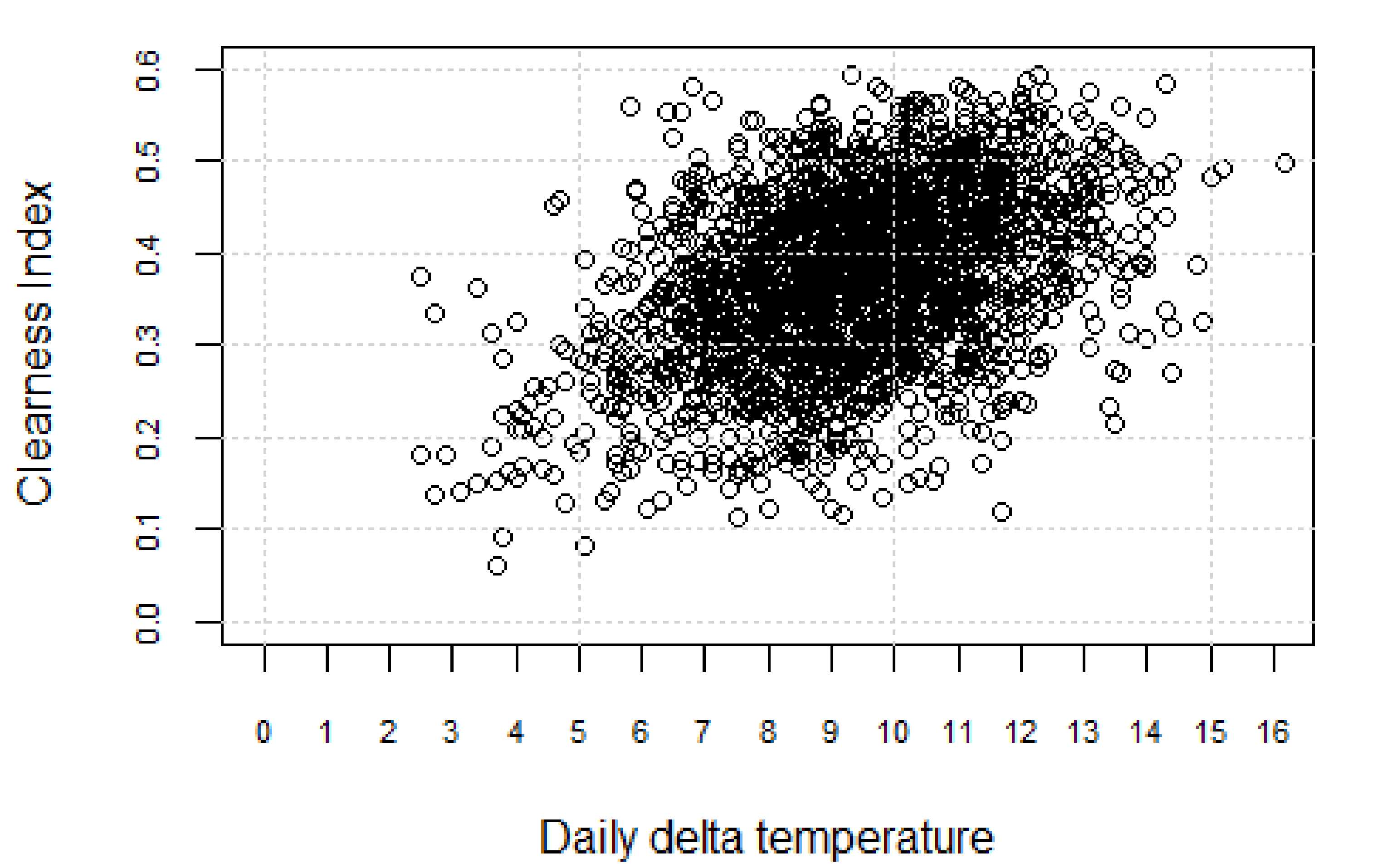
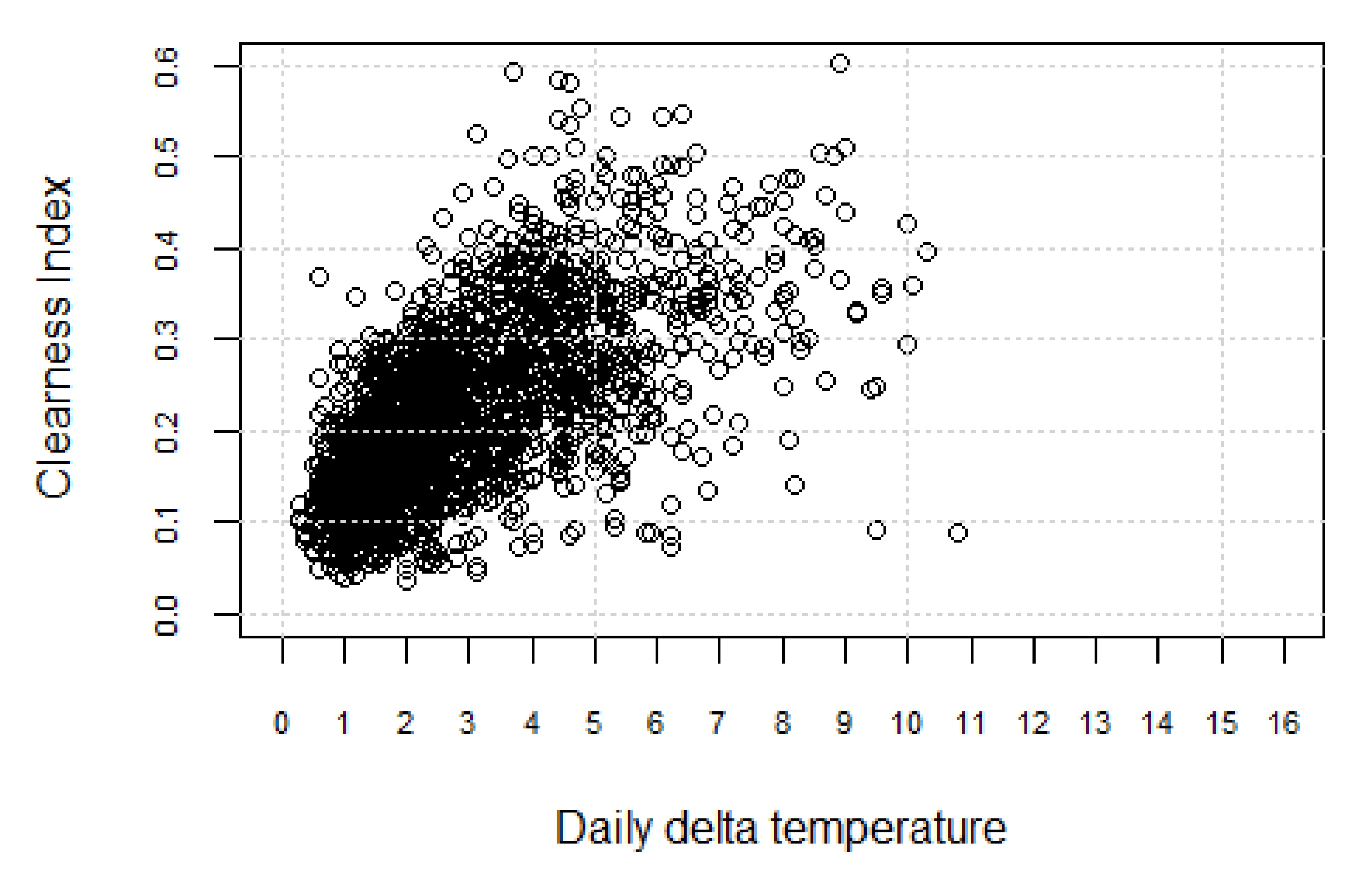
3.2.1. Model Development
3.2.2. Performance
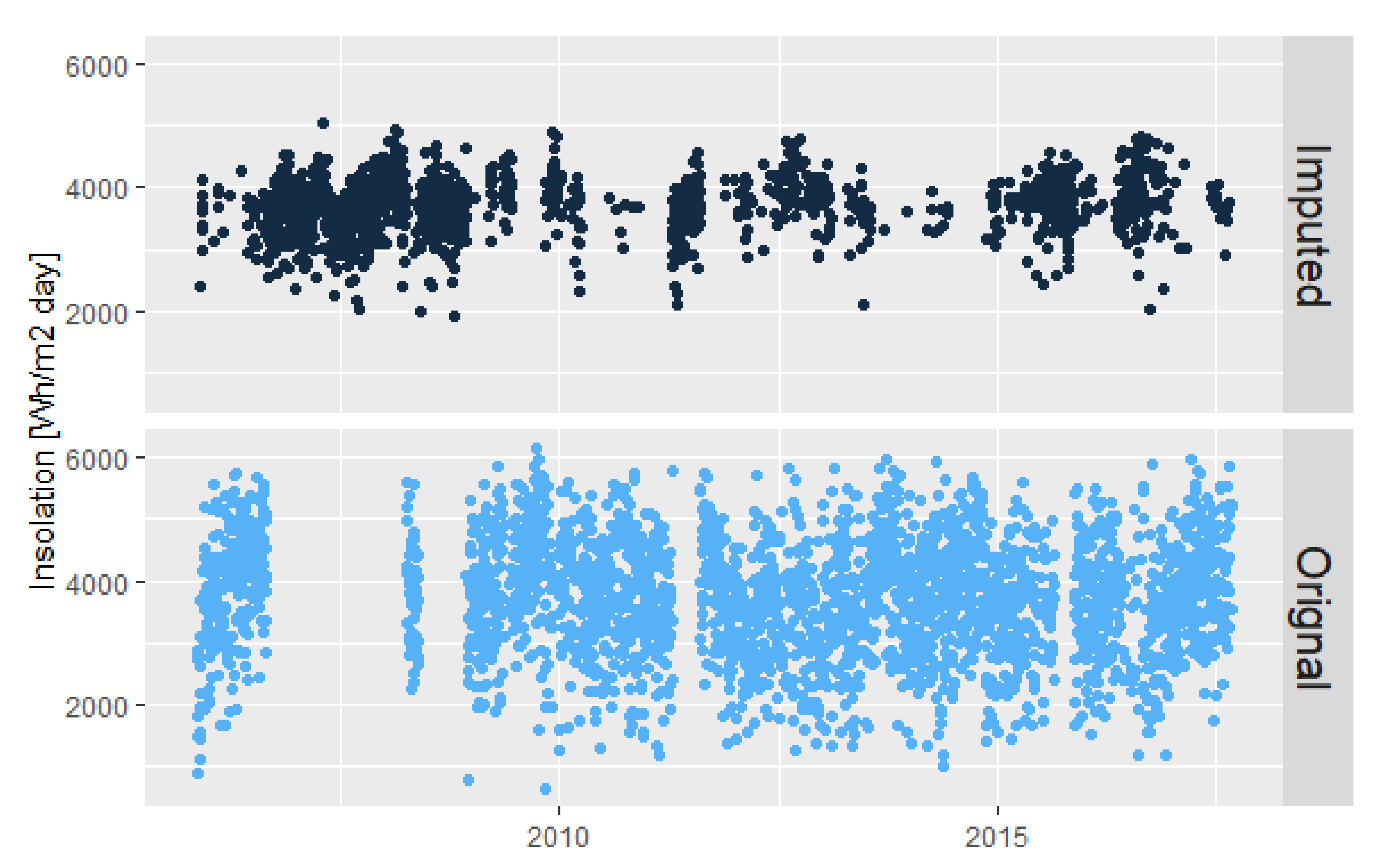
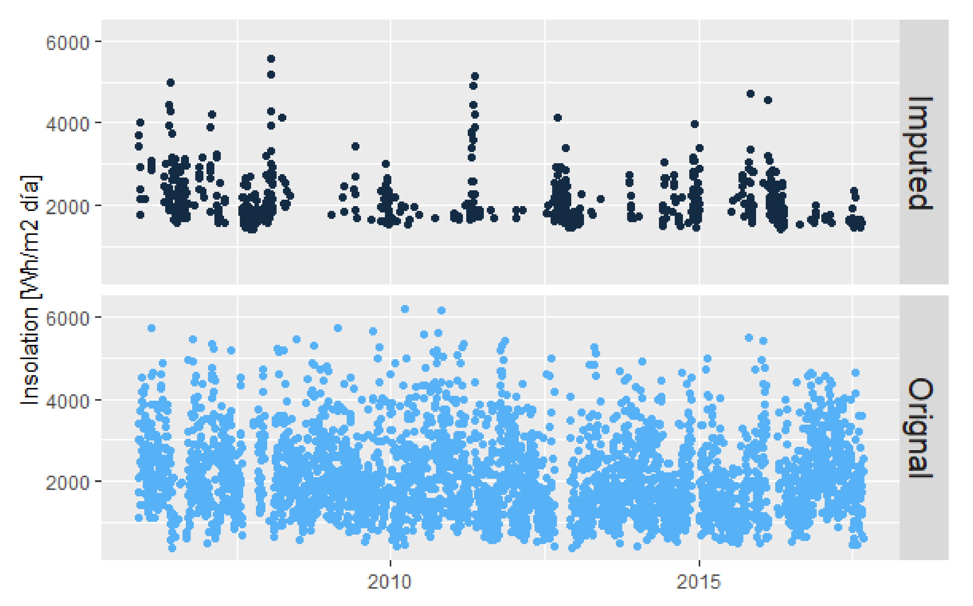
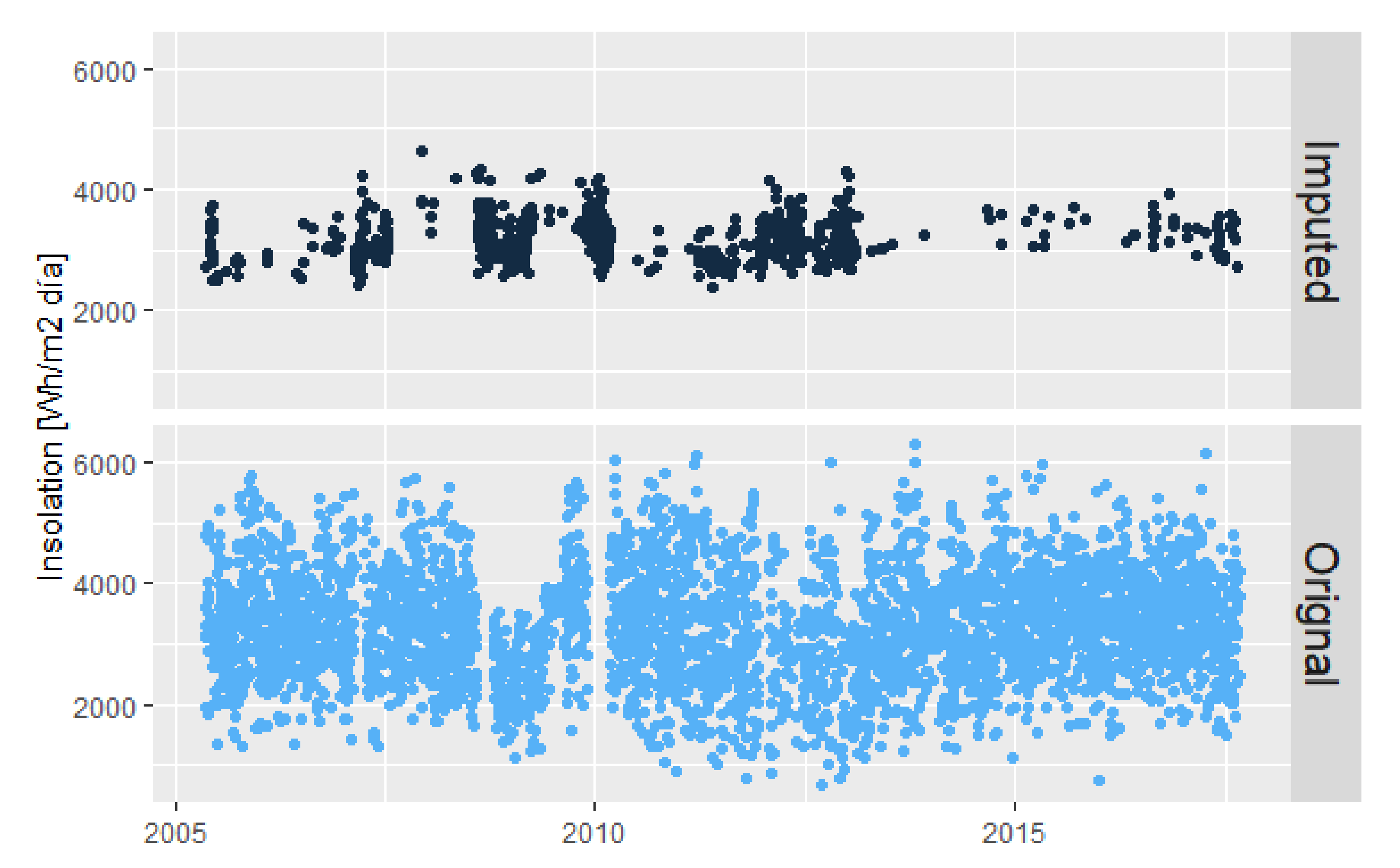
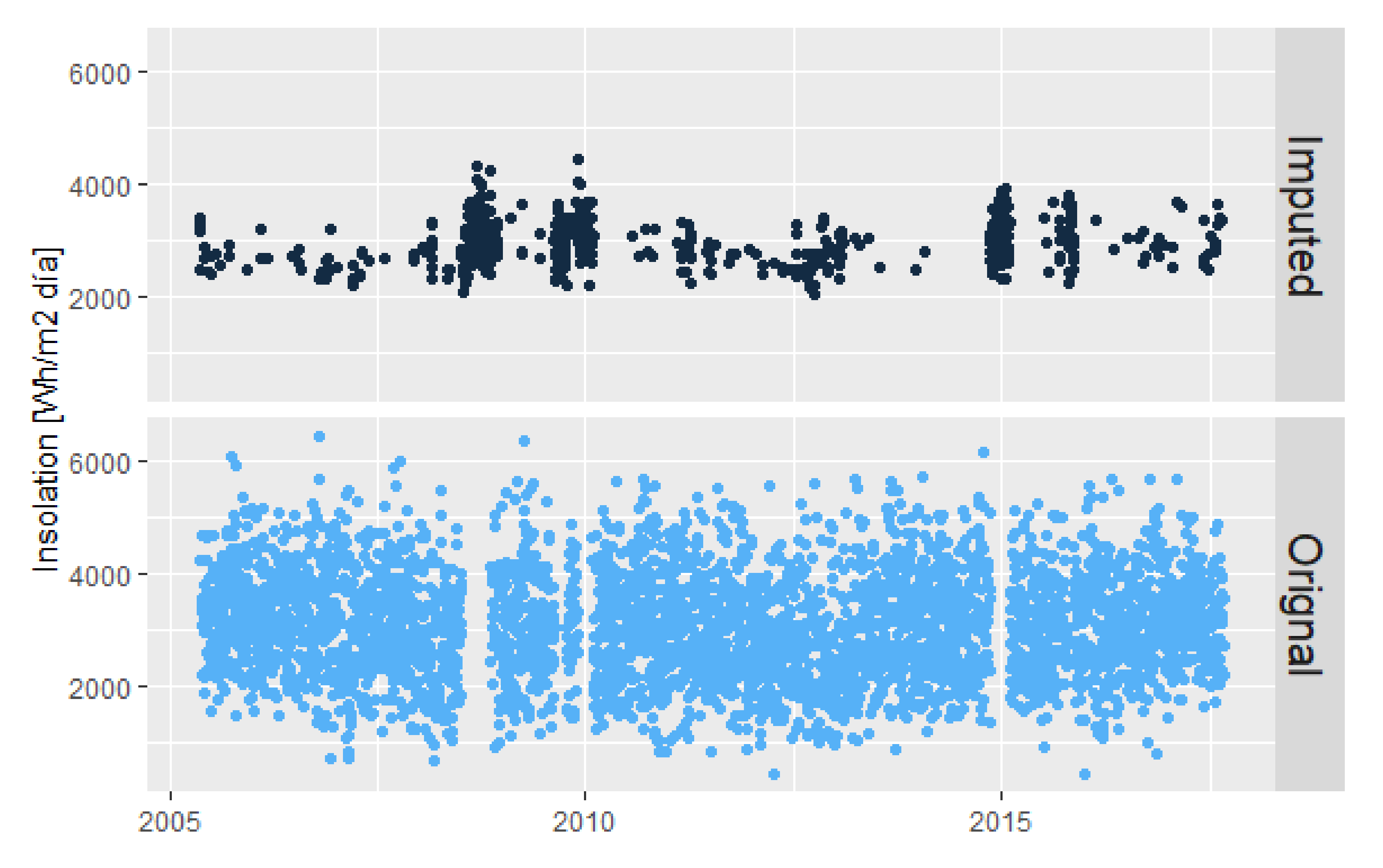
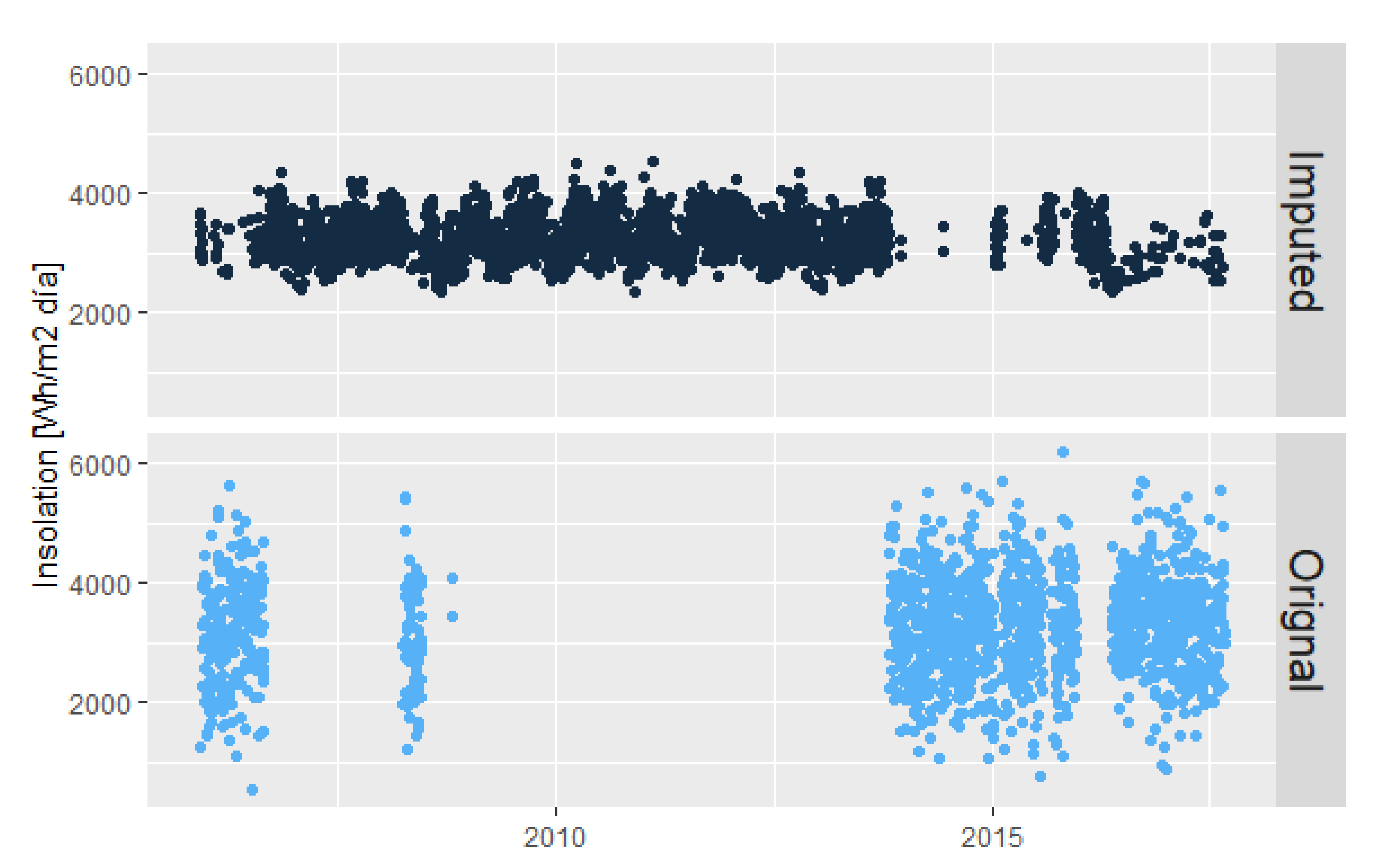
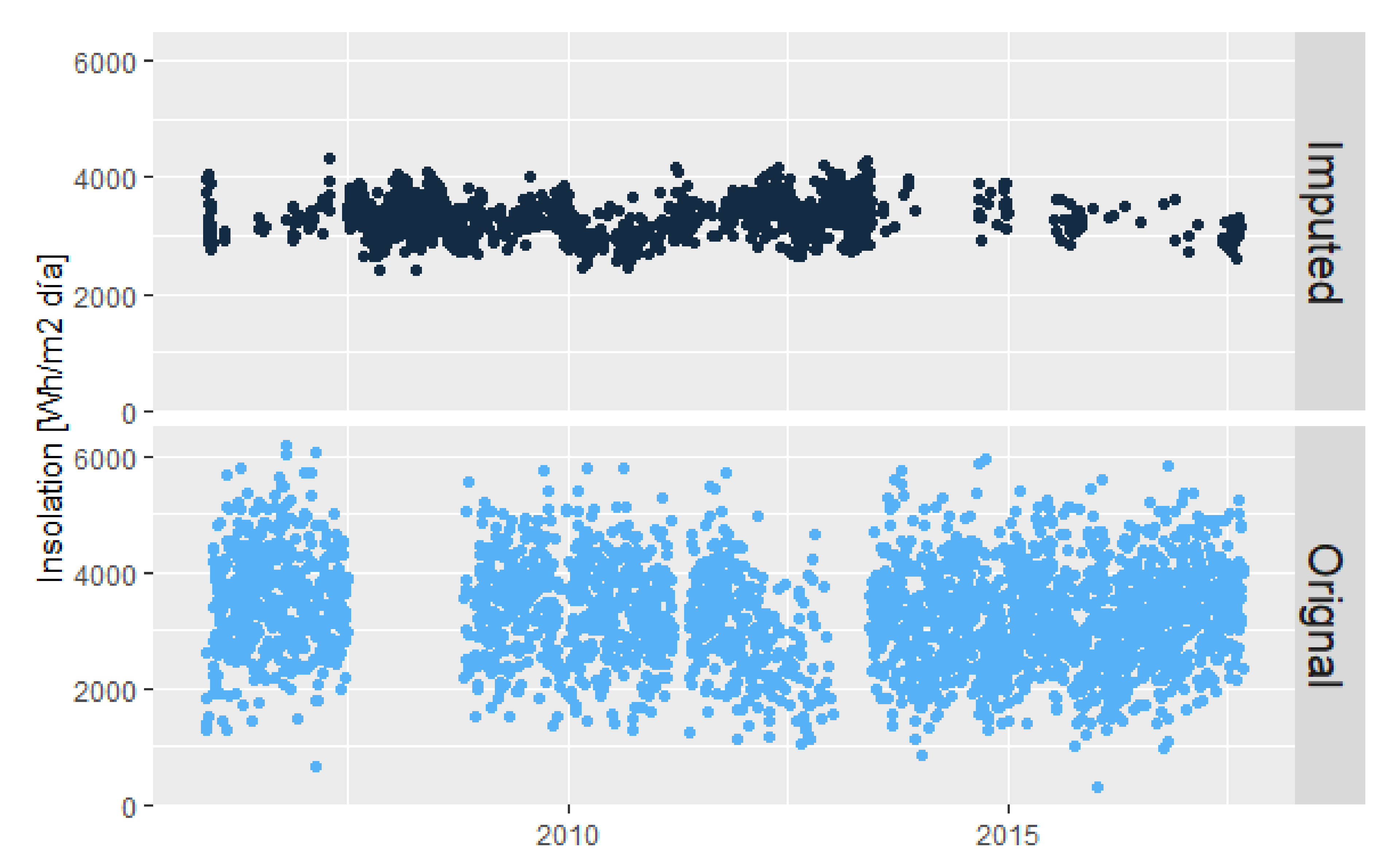
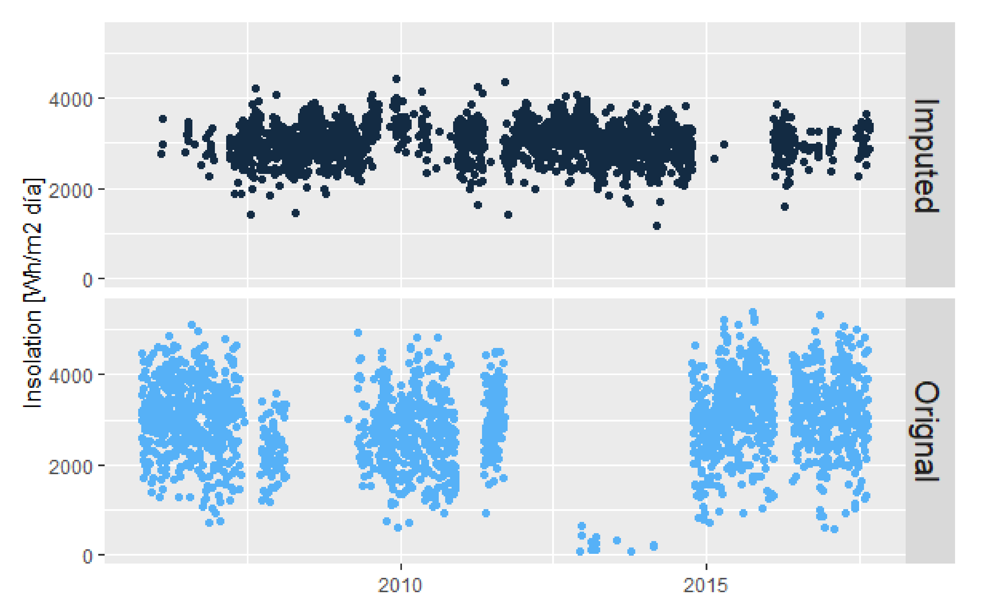
3.3. Imputation of Daily Solar Insolation Data
4. Conclusions
Author Contributions
Funding
Institutional Review Board Statement
Informed Consent Statement
Data Availability Statement
Acknowledgments
Conflicts of Interest
Nomenclature
| , , | Empirical coefficients |
| Global horizontal insolation | |
| Daily extraterrestrial solar irradiance | |
| Hourly extraterrestrial solar irradiance | |
| Hourly clear-sky global solar irradiance | |
| Hourly clear-sky global solar irradiance at time | |
| Global solar irradiance at time | |
| Solar constant | |
| Clearness index | |
| Hourly measured temperature | |
| Maximum daily temperature | |
| Mean daily temperature | |
| Minimum daily temperature | |
| Ratio between the daily minimum and maximum temperature | |
| Difference between the daily maximum and minimum temperature | |
| Latitude | |
| Solar declination | |
| Sunset hour angle | |
| Julian day | |
| Solar altitude | |
| Atmospheric transmittance |
References
- Hassan, G.E.; Youssef, M.E.; Mohamed, Z.E.; Ali, M.A.; Hanafy, A.A. New Temperature-based Models for Predicting Global Solar Radiation. Appl. Energy 2016, 179, 437–450. [Google Scholar] [CrossRef]
- Bakirci, K. Models of solar radiation with hours of bright sunshine: A review. Renew. Sustain. Energy Rev. 2009, 13, 2580–2588. [Google Scholar] [CrossRef]
- Jahani, B.; Dinpashoh, Y.; Raisi, A. Evaluation and development of empirical models for estimating daily solar radiation. Renew. Sustain. Energy Rev. 2017, 73, 878–891. [Google Scholar] [CrossRef]
- Besharat, F.; Dehghan, A.A.; Faghih, A.R. Empirical models for estimating global solar radiation: A review and case study. Renew. Sustain. Energy Rev. 2013, 21, 798–821. [Google Scholar] [CrossRef]
- Benson, R.B.; Paris, M.V.; Sherry, J.E.; Justus, C.G. Estimation of daily and montly direct, diffuse and global solar radiation from sunshine duration measurements. Sol. Energy 1984, 32, 523–535. [Google Scholar] [CrossRef]
- Akinoglu, B. Recent Advances in the Relations between Bright Sunshine Hours and Solar Irradiation. In Modeling Solar Radiation at the Earth’s Surface; Springer: Berlin/Heidelberg, Germany, 2008; pp. 115–143. [Google Scholar] [CrossRef]
- Almorox, J.; Hontoria, C.; Benito, M. Models for obtaining daily global solar radiation with measured air temperature data in Madrid (Spain). Appl. Energy 2011, 88, 1703–1709. [Google Scholar] [CrossRef]
- Fan, J.; Chen, B.; Wu, L.; Zhang, F.; Lu, X.; Xiang, Y. Evaluation and development of temperature-based empirical models for estimating daily global solar radiation in humid regions. Energy 2018, 144, 903–914. [Google Scholar] [CrossRef]
- Hargreaves, G.H.; Samani, Z.A. Estimating Potential Evapotranspiration. J. Irrig. Drain. Div. 1982, 108, 225–230. [Google Scholar] [CrossRef]
- Bristow, K.L.; Campbell, G.S. On the relationship between incoming solar radiation and daily maximum and minimim temperature. Agric. For. Meteorol. 1984, 31, 159–166. [Google Scholar] [CrossRef]
- Chen, J.; Liu, H.; Wu, W.; Xie, D. Estimation of monthly solar radiation from measured temperatures using support vector machines—A case study. Renew. Energy 2011, 36, 413–420. [Google Scholar] [CrossRef]
- Li, H.; Cao, F.; Wang, X.; Ma, W. A Temperature-Based Model for Estimating Monthly Average Daily Global Solar Radiation in China. Sci. World J. 2014, 2014, 128754. [Google Scholar] [CrossRef] [Green Version]
- Quansah, E.; Amekudzi, L.K.; Preko, K.; Aryee, J.; Boakye, O.R.; Boli, D.; Salifu, M.R. Empirical Models for Estimating Global Solar Radiation over the Ashanti Region of Ghana. J. Sol. Energy 2014, 2014, 897970. [Google Scholar] [CrossRef] [Green Version]
- Dos Santos, C.M.; De Souza, J.L.; Ferreira, R.A., Jr.; Tiba, C.; de Melo, R.O.; Lyra, G.B.; Teodoro, I.; Lyra, G.B.; Lemes, M.A.M. On modeling global solar irradiation using air temperature for Alagoas State, Northeastern Brazil. Energy 2014, 71, 388–398. [Google Scholar] [CrossRef]
- Rivero, M.; Orozco, S.; Sellschopp, F.S.; Loera-Palomo, R. A new methodology to extend the validity of the Hargreaves-Samani model to estimate global solar radiation in different climates: Case study Mexico. Renew. Energy 2017, 114, 1340–1352. [Google Scholar] [CrossRef]
- Jamil, B.; Akhtar, N. Comparison of empirical models to estimate monthly mean di ff use solar radiation from measured data: Case study for humid-subtropical climatic region of India. Renew. Sustain. Energy Rev. 2017, 77, 1326–1342. [Google Scholar] [CrossRef]
- Instituto Geográfico Agustín Codazzi—IGAC. Nariño Características Geográficas; Imprenta Nacional de Colombia: Bogotà, Colombia, 2014.
- Martínez, A.G. Nariño: Departamento de Nariño Colombia—Informacion Detallada Nariño Colombia 2018. Available online: https://www.todacolombia.com/departamentos-de-colombia/narino.html (accessed on 2 October 2018).
- Gobernación de Nariño. Plan participativo de Desarrollo Departamental. Plan Desarro. Dep. Nariño 2016, 255. [Google Scholar] [CrossRef]
- Corponariño. Plan de Gestion Ambiental Regional 2002–2012; San Juan de Pasto, Colombia. 2001. Available online: https://www.google.com.hk/url?sa=t&rct=j&q=&esrc=s&source=web&cd=&ved=2ahUKEwj3msf58Jv0AhVyk1YBHWhcB_0QFnoECAYQAQ&url=http%3A%2F%2Fcorponarino.gov.co%2Fexpedientes%2Fpgar20022012%2Fpgar2002-2012.pdf&usg=AOvVaw0oNP5AtXgL_y7Cn00TvEic (accessed on 1 November 2021).
- Estévez, J.; Gavilán, P.; Giráldez, J.V. Guidelines on validation procedures for meteorological data from automatic weather stations. J. Hydrol. 2011, 402, 144–154. [Google Scholar] [CrossRef] [Green Version]
- AENOR. Redes de Estaciones Meteorológicas Automáticas: Directrices Para la Validación de Registros Meteorológicos Procedentes de Redes de Estaciones Automáticas. Validación en Tiempo Real. 2004. Available online: https://www.une.org/encuentra-tu-norma/busca-tu-norma/norma?c=N0031912 (accessed on 1 November 2021).
- Kipp, Z. Instruction Manual Pyranometer/Albedometer CM11 e CM14 2000. Available online: https://www.google.com.hk/url?sa=t&rct=j&q=&esrc=s&source=web&cd=&ved=2ahUKEwi-7ovK8pv0AhVFp1YBHYzaBMkQFnoECAUQAQ&url=https%3A%2F%2Fs.campbellsci.com%2Fdocuments%2Fus%2Fmanuals%2Fkippzonen_manual_cmp-series.pdf&usg=AOvVaw0V6zEJQuWa8A1q7zAXlzJW (accessed on 1 November 2021).
- Şen, Z. Solar Energy Fundamentals and Modeling Techniques; Springer: Berlin/Heidelberg, Germany, 2008. [Google Scholar] [CrossRef]
- Serrano, A.; Sanchez, G.; Cancillo, M.L. Correcting daytime thermal offset in unventilated pyranometers. J. Atmos. Ocean. Technol. 2015, 32, 2088–2099. [Google Scholar] [CrossRef]
- Herrera-Grimaldi, P.; García-Marín, A.P.; Estévez, J. Multifractal analysis of diurnal temperature range over Southern Spain using validated datasets. Chaos 2019, 29, 063105. [Google Scholar] [CrossRef] [PubMed]
- Paulescu, M. Solar Irradiation via Air Temperature Data. In Modeling Solar Radiation at the Earth Surface; Badescu, V., Ed.; Springer: Berlin/Heidelberg, Germany, 2008; pp. 175–193. [Google Scholar]
- Meza, F.; Varas, E. Estimation of mean monthly solar global radiation as a function of temperature. Agric. For. Meteorol. 2000, 100, 231–241. [Google Scholar] [CrossRef]
- Moreno, A.; Gilabert, M.A.; Martínez, B. Mapping daily global solar irradiation over Spain: A comparative study of selected approaches. Sol. Energy 2011, 85, 2072–2084. [Google Scholar] [CrossRef]
- Ul Rehman Tahir, Z.; Hafeez, S.; Asim, M.; Amjad, M.; Farooq, M.; Azhar, M.; Amjad, G.M. Estimation of daily diffuse solar radiation from clearness index, sunshine duration and meteorological parameters for different climatic conditions. Sustain. Energy Technol. Assess. 2021, 47, 101544. [Google Scholar] [CrossRef]
- Mujabar, S.; Chintaginjala Venkateswara, R. Empirical models for estimating the global solar radiation of Jubail Industrial City, the Kingdom of Saudi Arabia. SN Appl. Sci. 2021, 3, 95. [Google Scholar] [CrossRef]
- Samani, Z. Estimating Solar Radiation and Evapotranspiration Using Minimum Climatological Data. J. Irrig. Drain. Eng. 2000, 126, 265–267. [Google Scholar] [CrossRef]
- Allen, R.G.; Pereira, L.S.; Raes, D.; Smith, M. Crop Evapotranspiration-Guidelines for Computing Crop Water Requirements—FAO Irrigation and Drainage Paper 56; FAO: Rome, Italy, 1998. [Google Scholar]
- Allen, R.G. Self-Calibrating Method for Estimating Solar Radiation From Air Temperature. J. Hydrol. Eng. 1997, 2, 56–67. [Google Scholar] [CrossRef]
- Goodin, D.G.; Hutchinson, J.M.S.; Vanderlip, R.L.; Knapp, M.C.; Goodin, D.G. Estimating Solar Irradiance for Crop Modeling Using Daily Air Temperature Data. Agroclimatology 1999, 91, 845–851. [Google Scholar] [CrossRef]
- Okundamiya, M.S.; Nzeako, A.N. Empirical Model for Estimating Global Solar Radiation on Horizontal Surfaces for Selected Cities in the Six Geopolitical Zones in Nigeria. J. Control. Sci. Eng. 2011, 2011, 805–812. [Google Scholar] [CrossRef] [Green Version]
- Nwokolo, S.C.; Ogbulezie, J.C. A quantitative review and classification of empirical models for predicting global solar radiation in West Africa. Beni-Suef Univ. J. Basic Appl. Sci. 2018, 7, 367–396. [Google Scholar] [CrossRef]
- Agami Reddy, T. Applied Data Analysis and Modelling for Energy Engineers and Scientists; Springer: London, UK, 2011. [Google Scholar] [CrossRef]
- Moon, S.H.; Kim, Y.H. An improved forecast of precipitation type using correlation-based feature selection and multinomial logistic regression. Atmos. Res. 2020, 240, 104928. [Google Scholar] [CrossRef]
- Kleinbaum, D.G.; Klein, M. Logistic Regression: A Self-Learning Text; Springer: Berlin/Heidelberg, Germany, 2010. [Google Scholar] [CrossRef]
- Manning, R.L. Logit regressions with continuous dependent variables measured with error. Appl. Econ. Lett. 1996, 3, 183–184. [Google Scholar] [CrossRef]
- Harrenll, F.E. Regression Modeling Strategies: With Applications to Linear Models, Logistic Regression, and Survival Analysis; Springer: Berlin/Heidelberg, Germany, 2015; Volume 13. [Google Scholar] [CrossRef]
- Casella, G.; Berger, R.L. Statistical Inference, 2nd ed.; Thomson: Toronto, ON, Canada, 2002. [Google Scholar]
- Mayer, D.G.; Butler, D.G. Statistical validation. Ecol. Model. 1993, 68, 21–32. [Google Scholar] [CrossRef]
- Gueymard, C.A. A review of validation methodologies and statistical performance indicators for modeled solar radiation data: Towards a better bankability of solar projects. Renew. Sustain. Energy Rev. 2014, 39, 1024–1034. [Google Scholar] [CrossRef]
- Li, J.; Heap, A.D. A review of comparative studies of spatial interpolation methods in environmental sciences: Performance and impact factors. Ecol. Inform. 2011, 6, 228–241. [Google Scholar] [CrossRef]
- Blumthaler, M. Solar Radiation of the High Alps. In Plants in Alpine Regions Cell Physiology of Adaptation and Survival Strategies; Lütz, C., Ed.; Springer: New York, NY, USA, 2012; pp. 11–20. [Google Scholar] [CrossRef]
- Cabrera, O.; Champutiz, B.; Calderon, A.; Pantoja, A. Landsat and MODIS satellite image processing for solar irradiance estimation in the department of Narino-Colombia. In Proceedings of the 2016 21st Symposium on Signal Processing, Images and Artificial Vision, STSIVA 2016, Bucaramanga, Colombia, 31 August–2 September 2016; pp. 1–6. [Google Scholar] [CrossRef]


| Name | Latitude | Longitude | Altitude | Period | Region |
|---|---|---|---|---|---|
| Biotopo | 1.41 | −78.28 | 512 | 2005–2017 | Pacific |
| Altaquer * | 1.56 | −78.09 | 101 | 2013–2014 | Pacific |
| Granja el Mira | 1.55 | −78.70 | 16 | 2016–2017 | Pacific |
| Cerro Páramo | 0.84 | −77.39 | 3577 | 2005–2017 | Amazon |
| La Josefina | 0.93 | −77.48 | 2449 | 2005–2017 | Andean |
| Viento Libre | 1.62 | −77.34 | 1005 | 2005–2017 | Andean |
| Universidad de Nariño | 1.23 | −77.28 | 2626 | 2005–2017 | Andean |
| Botana | 1.16 | −77.27 | 2820 | 2005–2017 | Andean |
| El Paraiso | 1.07 | −77.63 | 3120 | 2005–2017 | Andean |
| Guapi ** | 2.57 | −77.89 | 42 | 2005–2017 | Pacific |
| Name | Latitude | Longitude | Altitude | Period | Region |
|---|---|---|---|---|---|
| CCCP del Pacífico | 1.82 | −78.73 | 1 | 2005–2017 | Pacific |
| Altaquer | 1.56 | −78.09 | 1010 | 2005–2013 | Pacific |
| Granja el Mira | 1.55 | −78.69 | 16 | 2005–2017 | Pacific |
| Obonuco | 1.19 | −77.30 | 2710 | 2005–2015 | Andean |
| Apto. Antonio Nariño | 1.39 | −77.29 | 1796 | 2005–2017 | Andean |
| San Bernardo | 1.53 | −77.03 | 2190 | 2005–2017 | Andean |
| Taminango | 1.55 | −77.27 | 1875 | 2005–2017 | Andean |
| Común el automática | 0.93 | −77.63 | 3141 | 2007–2017 | Andean |
| Apto. San Luis | 0.86 | −77.67 | 2961 | 2005–2017 | Andean |
| Bombona | 1.18 | −77.46 | 1493 | 2005–2017 | Andean |
| Tanama | 1.37 | −77.58 | 1500 | 2005–2017 | Andean |
| Sindagua | 1.11 | −77.39 | 2800 | 2005–2017 | Andean |
| Barbacoas | 1.67 | −78.13 | 32 | 2005–2012 | Pacific |
| Monopamba | 0.99 | −77.15 | 2719 | 2006–2016 | Amazon |
| El Encano | 1.15 | −77.16 | 2830 | 2005–2017 | Andean |
| Chimayoy | 1.26 | −77.28 | 2745 | 2005–2014 | Andean |
| Region Type | |
|---|---|
| 0.16 | Arid and semi-arid |
| 0.17 | Interior regions |
| 0.19 | Coastal regions |
| 0.10—0.09 | Humid climates |
| Day Type | |
|---|---|
| Cloudy/Overcast | |
| Partially cloudy | |
| Sunny | |
| Very sunny |
| Measurement | Definition | |
|---|---|---|
| Mean of percent error (MPE) | Values close to zero indicate a better model and suggest that the ratio of the standard deviation of the measured and computed value is near one. | |
| Mean absolute error (MAE) | The average vertical distance between each predicted and observed point. | |
| Root mean square error (RMSE) | This provides a measure of the error size but is sensitive to outlier values because the measure gives more weight to large errors. | |
| Mean bias error (MBE) | This measure provides information on the model’s long-term performance when the model includes a systematic error that presents overestimated or underestimated predictors. Low MBE values are desirable, although it should be noted that an overestimated dataset will cancel out another underestimated dataset. | |
| Standard Deviation of the residual (SD) | This measure shows the difference between the standard deviation of the predicted and observed datasets. | |
| Uncertainty at 95% | This is a measure of certainty confidence; a lower value is expected. |
| Name | Code | Data | Step 1 | Step 2 | Step 3 | Step 4 |
|---|---|---|---|---|---|---|
| Biotopo | 51025060 | 47,612 | 46,557 | 24,385 | 20,699 | 12,883 |
| Viento Libre | 52035040 | 77,424 | 67,709 | 40,777 | 26,835 | 12,311 |
| Universidad de Nariño | 52045080 | 98,452 | 93,338 | 72,715 | 37,481 | 21,033 |
| Cerro Páramo | 52055150 | 90,440 | 81,940 | 57,407 | 36,661 | 25,709 |
| La Josefina | 52055170 | 55,909 | 54,041 | 29,966 | 14,183 | 7427 |
| Botana | 52055210 | 98,928 | 90,777 | 51,416 | 38,327 | 20,847 |
| El Paraiso | 52055220 | 88,408 | 82,135 | 54,371 | 29,033 | 14,394 |
| Guapi | 53045040 | 78,773 | 72,708 | 49,039 | 22,452 | 12,747 |
| Average | 79,493 | 73,651 | 47,510 | 28,208 | 15,919 |
| Data Number per Day * | 1 | 2 | 3 | 4 | 5 | 6 | 7 | 8 | 9 | 10 | 11 | 12 | 13 | Total of Days | |
|---|---|---|---|---|---|---|---|---|---|---|---|---|---|---|---|
| Name | |||||||||||||||
| Biotopo | 13 ** | 16 | 15 | 19 | 30 | 49 | 104 | 190 | 350 | 528 | 622 | 207 | 6 | 2149 | |
| Viento Libre | 43 | 50 | 77 | 86 | 121 | 175 | 313 | 444 | 702 | 654 | 390 | 119 | 11 | 3185 | |
| Universidad de Nariño | 27 | 42 | 56 | 73 | 97 | 173 | 340 | 403 | 730 | 1014 | 778 | 308 | 63 | 4104 | |
| Cerro Páramo | 34 | 39 | 42 | 45 | 59 | 83 | 145 | 283 | 483 | 952 | 1080 | 362 | 160 | 3767 | |
| La Josefina | 109 | 71 | 22 | 24 | 25 | 57 | 78 | 195 | 293 | 386 | 274 | 134 | 6 | 1674 | |
| Botana | 16 | 20 | 26 | 43 | 82 | 142 | 246 | 469 | 798 | 1066 | 839 | 336 | 14 | 4097 | |
| El Paraiso | 55 | 83 | 110 | 137 | 158 | 205 | 285 | 364 | 614 | 787 | 514 | 149 | 13 | 3474 | |
| Guapi | 185 | 193 | 180 | 153 | 111 | 101 | 139 | 239 | 335 | 447 | 549 | 182 | 75 | 2889 | |
| Name | Cloudy | Partially High Cloudiness | Partially Low Cloudiness | Sunny | Very Sunny | Number of Days * |
|---|---|---|---|---|---|---|
| Biotopo | 760 | 1188 | 67 | 0 | 0 | 2015 |
| Viento Libre | 105 | 1458 | 1179 | 0 | 0 | 2745 |
| Universidad de Nariño | 243 | 2611 | 846 | 1 | 0 | 3701 |
| Cerro Páramo | 1380 | 1232 | 137 | 1 | 0 | 2793 |
| La Josefina | 88 | 991 | 271 | 1 | 0 | 1351 |
| Botana | 451 | 2704 | 711 | 2 | 0 | 3868 |
| El Paraiso | 167 | 1859 | 543 | 1 | 0 | 2570 |
| Guapi | 130 | 746 | 125 | 0 | 0 | 1001 |
| Average | 16.99% | 64.70% | 18.28% | 0.03% | 0.00% | 100% |
| Name | Code | Data | Step 1 | Step 2 | Step 3 |
|---|---|---|---|---|---|
| Biotopo | 51025060 | 52.848 | 47.268 | 46.436 | 24.385 |
| Viento Libre | 52035040 | 77.424 | 67.969 | 67.962 | 40.777 |
| Universidad de Nariño | 52045080 | 100.740 | 94.880 | 92.886 | 72.715 |
| Cerro Páramo | 52055150 | 91.850 | 76.280 | 69.410 | 57.407 |
| La Josefina | 52055170 | 55.728 | 52.867 | 52.707 | 29.966 |
| Botana | 52055210 | 98.952 | 91.077 | 91.047 | 51.416 |
| El Paraiso | 52055220 | 91.699 | 85.713 | 84.792 | 54.371 |
| Guapi | 53045040 | 84.371 | 81.014 | 71.598 | 49.039 |
| Data Number per Day * | 1 | 2 | 3 | 4 | 5 | 6 | 7 | 8 | 9 | 10 | 11 | 12 | Total of Days | |
|---|---|---|---|---|---|---|---|---|---|---|---|---|---|---|
| Name | ||||||||||||||
| Biotopo | 33 ** | 9 | 17 | 13 | 26 | 46 | 56 | 85 | 130 | 257 | 605 | 846 | 2123 | |
| Viento Libre | 79 | 68 | 91 | 91 | 94 | 120 | 124 | 192 | 264 | 500 | 873 | 696 | 3192 | |
| Universidad de Nariño | 74 | 26 | 24 | 31 | 47 | 71 | 113 | 198 | 309 | 599 | 1170 | 1379 | 4041 | |
| Cerro Páramo | 101 | 49 | 58 | 47 | 67 | 86 | 133 | 190 | 348 | 590 | 754 | 701 | 3124 | |
| La Josefina | 61 | 21 | 36 | 46 | 50 | 78 | 109 | 130 | 197 | 405 | 573 | 558 | 2264 | |
| Botana | 38 | 11 | 27 | 46 | 62 | 102 | 147 | 253 | 386 | 679 | 1114 | 1221 | 4086 | |
| El Paraiso | 74 | 42 | 65 | 67 | 92 | 102 | 155 | 236 | 373 | 541 | 915 | 909 | 3571 | |
| Guapi | 20 | 8 | 10 | 21 | 18 | 21 | 45 | 79 | 168 | 405 | 919 | 1349 | 3063 | |
| Bristow and Campbell | |||
| AWS | |||
| Biotopo | 0.5075 | 0.0735 | 1.1908 |
| Viento Libre | 0.5942 | 0.1499 | 0.8655 |
| Cerro Páramo | 0.5922 | 0.2595 | 0.6153 |
| Universidad de Nariño | 0.4893 | 0.3282 | 0.6568 |
| Botana | 0.6288 | 0.1964 | 0.6415 |
| Josefina | 0.6039 | 0.2563 | 0.5350 |
| Paraiso | 0.5850 | 0.3183 | 0.4818 |
| Guapi | 0.4471 | 0.1156 | 1.2478 |
| Hargreaves and Samani | |||
| AWS | |||
| Biotopo | 0.0970 | ||
| Viento Libre | 0.1248 | ||
| Cerro Páramo | 0.1340 | ||
| Universidad de Nariño | 0.1263 | ||
| Botana | 0.1169 | ||
| Josefina | 0.1138 | ||
| Paraiso | 0.1199 | ||
| Guapi | 0.1208 | ||
| Okundamiya and Nzeako | |||
| AWS | |||
| Biotopo | −0.1838 | −0.3871 | 0.0264 |
| Viento Libre | 0.0578 | −0.2666 | 0.0168 |
| Cerro Páramo | 0.1084 | −0.1572 | 0.0257 |
| Universidad de Nariño | 0.2679 | −0.2416 | 0.0112 |
| Botana | 0.0621 | −0.1547 | 0.0191 |
| Josefina | 0.1770 | −0.1589 | 0.0118 |
| Paraiso | 0.2617 | −0.1775 | 0.0100 |
| Guapi | 0.0717 | −0.5202 | 0.0228 |
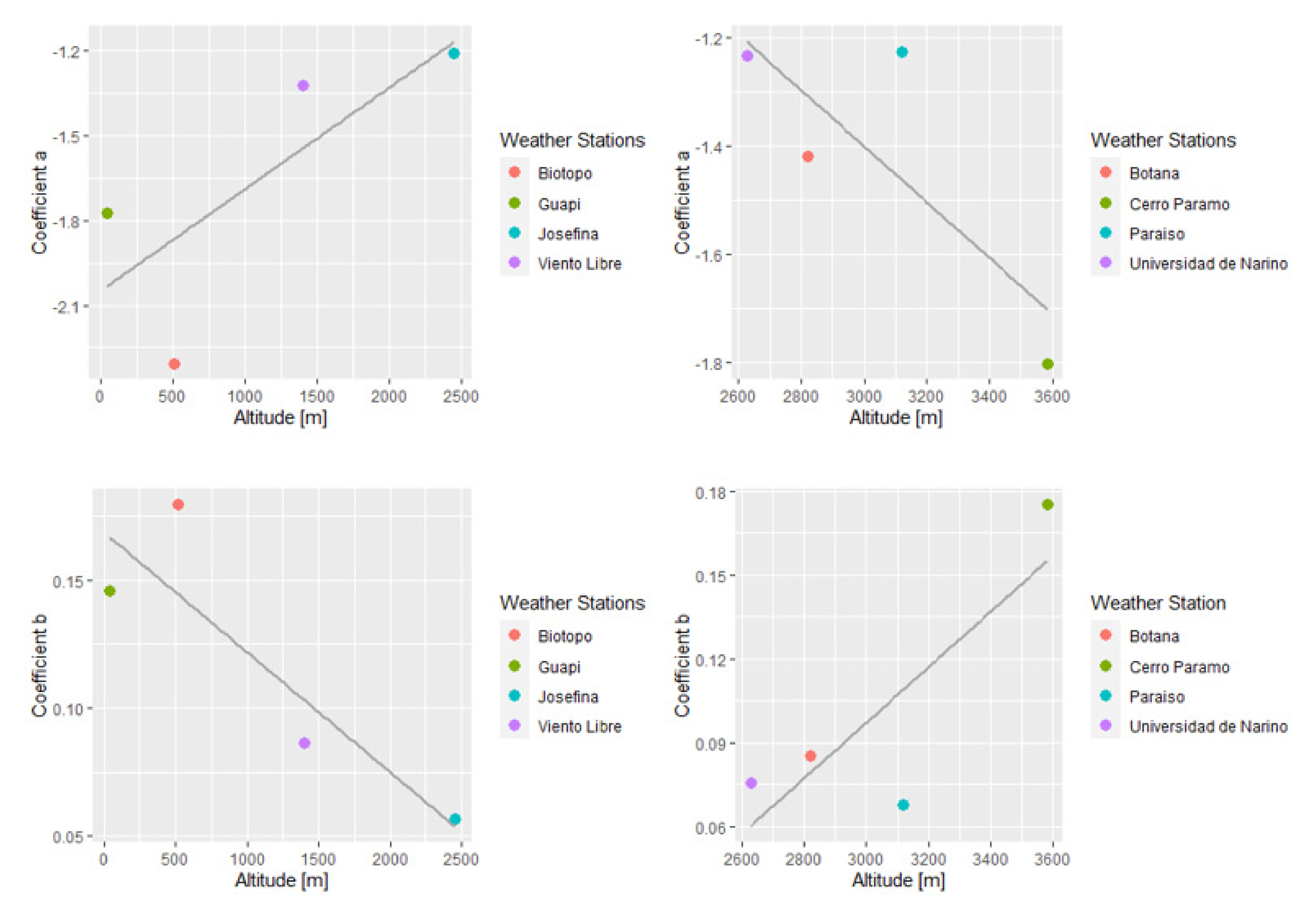
| Proposed model | |||
| AWS | |||
| Biotopo | −2.3058 | 0.1786 | |
| Viento Libre | −1.3499 | 0.0912 | |
| Cerro Páramo | −1.7914 | 0.1706 | |
| Universidad de Nariño | −1.2211 | 0.0747 | |
| Botana | −1.4489 | 0.0898 | |
| Josefina | −1.2299 | 0.0608 | |
| Paraiso | −1.1667 | 0.0607 | |
| Guapi | −1.8043 | 0.1495 | |
| AWS | BC | HS | ON | Proposed |
| Biotopo | 1.152,62 | 993,64 | 1.155,07 | 1.113,48 |
| Viento Libre | 1.086,47 | 1.080,72 | 1.110,62 | 1.077,35 |
| Cerro Páramo | 1.194,57 | 1.209,76 | 1.196,56 | 1.152,72 |
| Universidad de Nariño | 1.032,45 | 1.083,73 | 1.032,24 | 1.019,14 |
| Botana | 1.052,42 | 1.070,23 | 1.077,17 | 1.042,68 |
| Josefina | 1.009,00 | 1.066,18 | 999,28 | 984,75 |
| Paraiso | 930,82 | 990,32 | 938,02 | 921,32 |
| Guapi | 965,40 | 878,75 | 961,21 | 915,53 |
| AWS | BC | HS | ON | Proposed |
| Biotopo | 49,90 | 43,11 | 50,08 | 48,29 |
| Viento Libre | 29,21 | 29,05 | 29,86 | 28,97 |
| Cerro Páramo | 56,04 | 56,77 | 56,15 | 54,08 |
| Universidad de Nariño | 31,89 | 33,55 | 31,88 | 31,47 |
| Botana | 34,46 | 35,05 | 35,23 | 34,14 |
| Josefina | 31,29 | 33,06 | 30,99 | 30,53 |
| Paraiso | 27,82 | 29,58 | 28,04 | 27,54 |
| Guapi | 31,75 | 28,91 | 31,58 | 30,12 |
| AWS | BC | HS | ON | Proposed |
| Biotopo | −77,79 | −2,01 | −45,24 | −37,29 |
| Viento Libre | 162,63 | 163,13 | 167,77 | 160,23 |
| Cerro Páramo | 37,90 | 21,29 | 27,22 | 33,37 |
| Universidad de Nariño | 90,20 | 62,04 | 93,68 | 93,72 |
| Botana | 48,24 | 42,30 | 71,63 | 47,13 |
| Josefina | 5,28 | −20,58 | 16,92 | 22,18 |
| Paraiso | −23,17 | −42,52 | −15,89 | −14,98 |
| Guapi | −36,98 | −16,38 | −53,45 | −27,50 |
| AWS | BC | HS | ON | Proposed |
| Biotopo | 916,08 | 800,52 | 917,96 | 885,10 |
| Viento Libre | 863,76 | 861,64 | 883,10 | 862,86 |
| Cerro Páramo | 940,46 | 946,29 | 929,90 | 887,34 |
| Universidad de Nariño | 845,12 | 884,48 | 841,37 | 833,30 |
| Botana | 866,59 | 881,19 | 888,56 | 860,18 |
| Josefina | 769,70 | 830,06 | 767,58 | 760,43 |
| Paraiso | 757,02 | 806,64 | 760,64 | 748,67 |
| Guapi | 753,77 | 696,35 | 773,11 | 733,40 |
| AWS | BC | HS | ON | Proposed |
| Biotopo | 2.261,26 | 1.949,37 | 2.266,06 | 2.184,48 |
| Viento Libre | 2.130,26 | 2.118,99 | 2.177,61 | 2.112,38 |
| Cerro Páramo | 2.343,94 | 2.373,74 | 2.347,83 | 2.261,82 |
| Universidad de Nariño | 2.024,57 | 2.125,13 | 2.024,17 | 1.998,46 |
| Botana | 2.063,85 | 2.098,79 | 2.112,40 | 2.044,75 |
| Josefina | 1.978,59 | 1.941,90 | 1.959,53 | 1.931,04 |
| Paraiso | 1.825,23 | 1.941,90 | 1.839,34 | 1.806,59 |
| Guapi | 1.893,21 | 1.723,28 | 1.885,00 | 1.795,41 |
| AWS | BC | HS | ON | Proposed |
| Biotopo | 16,22% | 19,52% | 17,93% | 18,33% |
| Viento Libre | 15,34% | 15,32% | 15,39% | 15,18% |
| Cerro Páramo | 28,77% | 27,90% | 27,64% | 28,69% |
| Universidad de Nariño | 13,73% | 12,78% | 13,82% | 13,80% |
| Botana | 14,22% | 11,32% | 15,08% | 14,11% |
| Josefina | 12,24% | 20,51% | 12,52% | 12,70% |
| Paraiso | 8,24% | 7,70% | 8,59% | 8,51% |
| Guapi | 6,82% | 7,46% | 6,11% | 7,12% |
| AWS | BC | HS | ON | Proposed |
| Biotopo | 49,13% | 44,53% | 49,71% | 48,13% |
| Viento Libre | 30,09% | 29,99% | 30,46% | 29,94% |
| Cerro Páramo | 56,68% | 56,62% | 55,00% | 53,67% |
| Universidad de Nariño | 31,44% | 32,47% | 31,26% | 30,97% |
| Botana | 34,42% | 32,58% | 35,35% | 34,07% |
| Josefina | 30,83% | 37,42% | 30,74% | 30,56% |
| Paraiso | 26,75% | 28,29% | 26,91% | 26,47% |
| Guapi | 28,15% | 26,14% | 28,65% | 27,14% |
| AWS | Imputation |
|---|---|
| Biotopo | 2241 |
| Viento Libre | 1502 |
| Cerro Páramo | 749 |
| Universidad de Nariño | 686 |
| Botana | 585 |
| La Josefina | 2872 |
| Paraiso | 1369 |
| Guapi | 2277 |
Publisher’s Note: MDPI stays neutral with regard to jurisdictional claims in published maps and institutional affiliations. |
© 2021 by the authors. Licensee MDPI, Basel, Switzerland. This article is an open access article distributed under the terms and conditions of the Creative Commons Attribution (CC BY) license (https://creativecommons.org/licenses/by/4.0/).
Share and Cite
Hoyos-Gomez, L.S.; Ruiz-Mendoza, B.J. A New Empirical Approach for Estimating Solar Insolation Using Air Temperature in Tropical and Mountainous Environments. Appl. Sci. 2021, 11, 11491. https://doi.org/10.3390/app112311491
Hoyos-Gomez LS, Ruiz-Mendoza BJ. A New Empirical Approach for Estimating Solar Insolation Using Air Temperature in Tropical and Mountainous Environments. Applied Sciences. 2021; 11(23):11491. https://doi.org/10.3390/app112311491
Chicago/Turabian StyleHoyos-Gomez, Laura Sofía, and Belizza Janet Ruiz-Mendoza. 2021. "A New Empirical Approach for Estimating Solar Insolation Using Air Temperature in Tropical and Mountainous Environments" Applied Sciences 11, no. 23: 11491. https://doi.org/10.3390/app112311491
APA StyleHoyos-Gomez, L. S., & Ruiz-Mendoza, B. J. (2021). A New Empirical Approach for Estimating Solar Insolation Using Air Temperature in Tropical and Mountainous Environments. Applied Sciences, 11(23), 11491. https://doi.org/10.3390/app112311491