Article

Use of Deep Learning to Improve the Computational Complexity of Reconstruction Algorithms in High Energy Physics

by
Núria Valls Canudas
*,
Míriam Calvo Gómez
*,
Elisabet Golobardes Ribé
* and
Xavier Vilasis-Cardona
*
Data Science for the Digital Society (DS4DS) Research Group, Engineering Department, La Salle-Universitat Ramon Llull, Sant Joan de La Salle 42, 08022 Barcelona, Spain
*
Authors to whom correspondence should be addressed.
Appl. Sci. 2021, 11(23), 11467; https://doi.org/10.3390/app112311467
Submission received: 15 November 2021 / Revised: 28 November 2021 / Accepted: 1 December 2021 / Published: 3 December 2021
(This article belongs to the Special Issue Women in Artificial intelligence (AI))

Abstract

:
The optimization of reconstruction algorithms has become a key aspect in the field of experimental particle physics. Since technology has allowed gradually increasing the complexity of the measurements, the amount of data taken that needs to be interpreted has grown as well. This is the case with the LHCb experiment at CERN, where a major upgrade currently undergoing will considerably increase the data processing rate. This has presented the need to search for specific reconstruction techniques that aim to accelerate one of the most time consuming reconstruction algorithms in LHCb, the electromagnetic calorimeter clustering. Together with the use of deep learning techniques and the understanding of the current reconstruction algorithm, we propose a method that decomposes the reconstruction process into small parts that can be formulated as a cellular automaton. This approach is shown to benefit the generalized learning of small convolutional neural network architectures and also simplify the training dataset. Final results applied to a complete LHCb simulation reconstruction are compatible in terms of efficiency, and execute in nearly constant time with independence on the complexity of the data.

1. Introduction

In the field of high energy physics (HEP) there are many computational challenges regarding data. In most collider experiments the first step that needs to be done, when a collision happens inside a detector, is reconstructing the data. This process consists of an algorithm that transforms these data into information of what physical phenomena happened inside the detector, so that later on physicists can use it for a detailed analysis. The LHCb experiment at CERN [1] is not an exception. Due to the collision rate generated at the large hadron collider (LHC) accelerator [2], the throughput rate is so high that data cannot be stored before processing. In this case, together with all of the experiments at LHC, the reconstruction process of data has a very strict time constraint in order to obtain determinant information, to decide whether or not to store the data. More details on the overview of data processing are provided in Section 2.
At this point, optimization of reconstruction techniques is needed. Moreover, the vision of future upgrades [3] enhances the importance of developing scalable and flexible software methodologies. In the case of LHCb, the current time performance analysis of the reconstruction process points the calorimeter reconstruction as the second most computational expensive process, representing almost 25 % of the LHCb reconstruction time [4].
The LHCb electromagnetic calorimeter (ECAL) [5] is a subdetector designed to measure the energy of particles as they interact with the detector material. It has a rectangular shape of 7.8 × 6.3 m and is placed perpendicular to the accelerator beam pipe. Moreover, the purpose of the LHCb detector is to study heavy quark hadron decays. Those decays are known to produce particles coming out almost parallel to the beam pipe. Hence, the incident angle of particles striking the calorimeter is between 1° and 21°, with respect to the beam axis. The calorimeter detector structure is segmented into individual square-shaped modules that perform the energy measurement. Each module is made from lead absorber plates interspaced with scintillator tiles as active material and has a variable number of readout cells, depending on the position. To avoid confusion between the calorimeter cells and the cells from a cellular automaton, the calorimeter cells will be referred to as readout cells. The output data obtained from the calorimeter are the values from each readout cell concerning the accumulated energy deposited by incident particles in a single collision. Since particles may deposit energy in more than one readout cell, the energy deposits need to be reconstructed and clustered together with the ones belonging to the same particle.
Such a challenge, under very tight execution time constraints, invites one to think of neural network techniques that can provide the capability of learning complex problems and a fast inference. Considering its increasing popularity in recent years, there have been many improvements in the optimization of reconstruction algorithms. Specially, deep learning models are able to solve many complex issues at very high speeds, only at the cost of increasing the time and complexity of the training. However, most of these proposals approach the whole scenario at once, forcing the networks to process hundreds of thousands of data samples and understand their insights, to be able to provide a complete solution at the output. As problems become more challenging, deeper networks need to be trained with more data. Although nowadays, computational time is not an inconvenience in most cases, data acquisition is, especially in the HEP case, where data are simulated with time-consuming algorithms.
Beginning with the comprehension of the current implementation of the reconstruction algorithm, it is based on a cellular automaton [6]. Further details are provided in Section 3.1. Due to the typical square-shaped modular structure of the calorimeter, its geometry can be easily mapped into a two-dimensional grid. Therefore, the cellular automaton strategy has long been used in calorimeters for high energy physics [7,8]. Such a method provides an efficient reconstruction of the clusters, although the classical formulation of the cellular automaton requires several iterative processes along the readout cell values that are programmed as loops in the algorithm’s code. As this causes a strong dependency of the algorithm’s complexity on the number of clusters in the data, other approaches have attempted to avoid this dependency by exploiting the architecture similarities between cellular automata and neural networks [9,10]. However, these approaches focus on a proof of concept rather than providing a specific reconstruction solution for the LHCb calorimeter. Within recent years, the evolution of deep learning models has encouraged the use of image processing techniques for this challenge. An early stage project has shown promising results when approaching the LHCb calorimeter reconstruction with a deep neural network structure [11] based on the YOLOv3 network [12]. This particular case uses the order of 100,000 simulation samples to train a network of the order of 65 million parameters.
In this article, we propose a different formulation of the LHCb calorimeter reconstruction problem to improve the generalized learning of small deep learning architectures [13]. Those networks have been trained using artificially generated sets of data and preprocessed pieces of simulated LHCb data. With this methodology, we aim to have an efficient cluster reconstruction algorithm that performs at a nearly constant speed with independence of the event complexity.

2. Overview of Data Processing in Modern Particle Detectors

The physics analysis conducted in the modern HEP field starts with a particle accelerator. In the case of LHC, two streams of proton particles are accelerated up to 0.99999999 c and collide at four specific detection points. The LHCb experiment is placed in one of these four locations and has a subset of eight dedicated detectors to acquire data from the particles generated in the collisions. The electromagnetic calorimeter is one of them. Complementing the previous definition, the calorimeter detector’s general structure is segmented in three different rectangular-shaped regions, as can be seen in Figure 1.
Although all modules have the same size of 12 × 12 cm, the number of readout cells on a module depends on the region. The inner region is the closest to the accelerator pipe and has nine readout cells of 4 × 4 cm per module. It has the highest granularity among the three regions since it is the region with the highest occupancy of incident particles. The middle region surrounds the inner and has four readout cells of 6 × 6 cm per module, and the outer region has a single readout cell of 12 × 12 cm per module. Since the occupancy decreases with the distance from the accelerator pipe, the shape of the readout cells for middle and outer regions is increased following a trade-off between precision and cost. Regarding the size of the inner readout cells, it is calculated following the Molière radius. Therefore, a particle is expected to deposit all of its energy in one inner readout cell if it falls on its center. However, to ensure that all the energy from a particle is captured, and to simplify the reconstruction algorithm, the definition of a calorimeter cluster stands for a 3 × 3 block of readout cells around an energy peak. Some studies have been done regarding the cluster shapes [14] where 2 × 2 clusters show promising performance for high luminosity, although the 3 × 3 cluster is used as a base for masking other shapes on clusters. Therefore, for simplicity in the reconstruction process, the definition of 3 × 3 readout cell clusters is maintained through all the regions of the detector. Since in this approach we focus on improving the reconstruction performance rather than particle identification, we can only evaluate comparisons between the reconstruction results and simulation data.
In all particle physics experiments, data are not analyzed directly from the detector readout, what is called raw data. Instead, domain experts need information of what happened inside the detectors in order to make the physics’ analysis. This information is extracted through the reconstruction process. In the case of the calorimeter detector, a sample of raw data contains the list of readout cells that have an energy deposit from one collision. This needs to be reconstructed as all the groups of 3 × 3 readout cells with the energy, belonging to the same particle colliding into the calorimeter. Up until now, the amount of data generated by all the detectors at LHCb reached the order of 35 GB/s. However, the processing rate of each datum sample was decreased by a factor 40 to a throughput of 1 MHz using a hardware selector known as level 0 trigger [15]. In the upcoming upgrade of the experiment, the data processing rate is going to increase to 30 MHz, meaning the full 35 GB/s will be processed. Since this throughput rate cannot be stored with current technology, the trigger system will be upgraded into a full software trigger called the high level trigger (HLT), where complete data reconstruction needs to take place. Even so, since the number of collisions will also increase in the upgrade, the occupancy of the LHCb detector is going to increase in a factor five. This enhances the need to optimize and accelerate the current reconstruction algorithms in order to fit in the processing time constraints and throughput rate of the HLT.
At the time of building and testing reconstruction algorithms, there is no point in working with raw data from the detector, since there is no “truth information” of the particles that generated the raw sample. Instead, simulation data are produced using the Monte Carlo method, where particles are simulated together with its interaction with the detector. With these simulations, the reconstruction algorithms have a supervised set of data to compare the reconstruction output to the real particles impacting the detector.

3. Methods

In this section, the proposal is explained in detail, starting with an explanation of the fundamental principles applied.

3.1. Fundamentals

The current implementation for data reconstruction in the LHCb calorimeter consists of a cellular automaton based clustering [6]. A cellular automaton (CA) [16] is a computational system used to describe the evolution of a discrete system under a set of rules through discrete steps in time. The system is defined as a grid of cells of any dimension where each cell can have a finite number of states. At each step of time, every cell updates simultaneously its own state depending on the state of its neighbor cells following a defined set of rules.
Moving forward to the cluster reconstruction, the algorithm can be segmented into three different steps. The first one consists of a local maxima finder algorithm to identify the potential centers of particle clusters. The second step is the proper cellular automaton, which iteratively tags each of the cells to the closest maximum and enhances those cells that may have contributions from more than one cluster. The final step consists of an iterative algorithm that resolves those particular cases, from now on known as overlapping cells.
Each of the three steps mentioned are indeed iterative algorithms that analyze the grid of calorimeter readout cells using a set of specific rules to give a certain condition in the end. Going further, all steps can be defined as a CA. Given the universality theorem of the CAs, there exists a set of rules and a set of states that can model the behavior of the mentioned algorithms as a dynamic system.
In this article, we propose modeling each of the three steps of the reconstruction process as a CA with an ad-hoc formulation. With this we can benefit from the fact that convolutional neural networks have been proven to learn the generalized rules of cellular automata [17]. Hence, we will train a convolutional neural network with the rules of each of the reconstruction steps to build a pipeline of networks that perform the full reconstruction of the calorimeter.

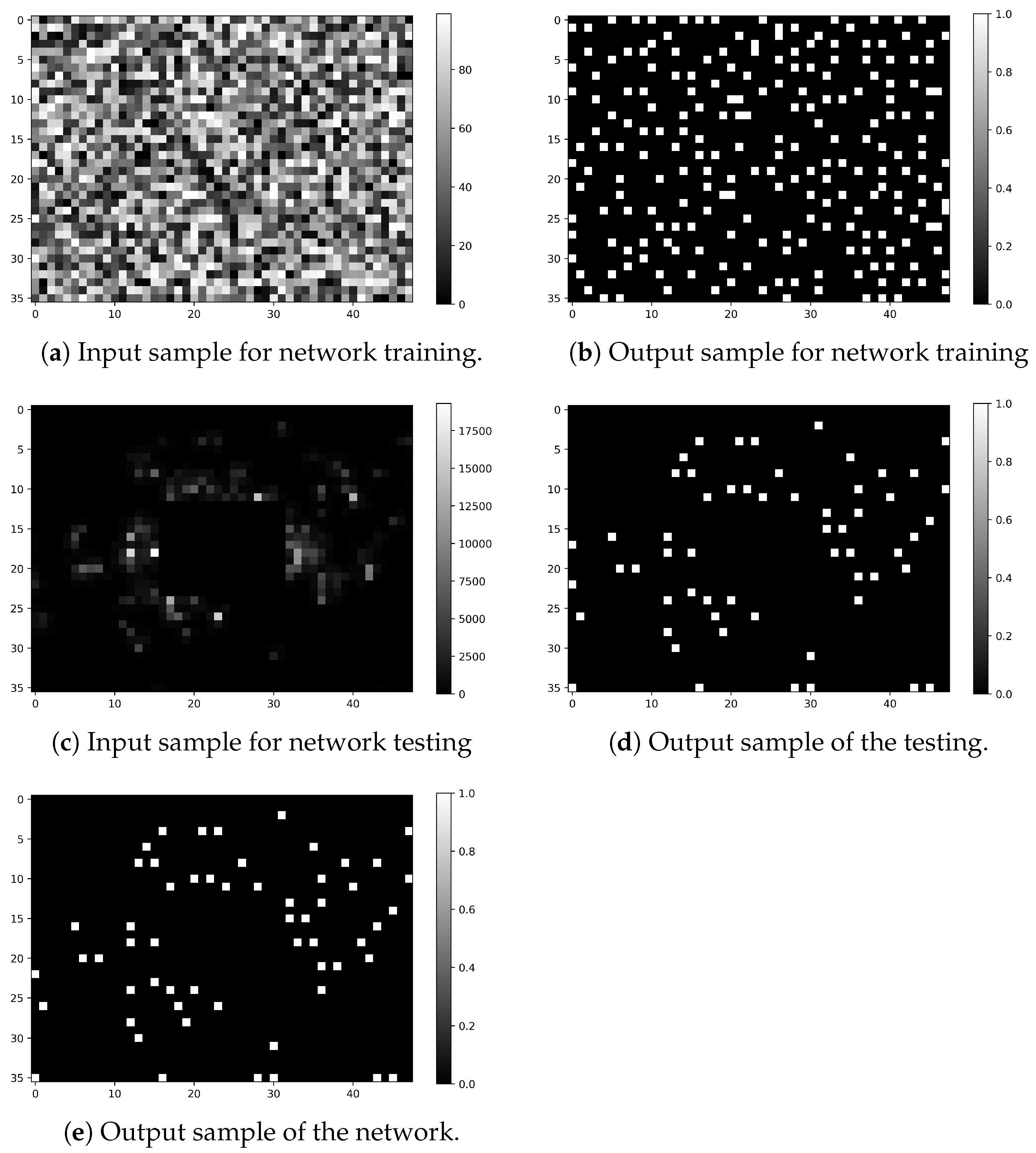
3.2. Local Maxima Formulation

Starting with the local maxima finder, we want to identify cells that are a local maxima among the others. Hence, its cellular automata characteristics can be defined as follows:
  • States: two. One (1) if the cell is a maximum and zero (0) otherwise.
  • Neighborhood: eight cells. In order to check if it is a local maxima, the surrounding cells at distance one need to be checked. In a two-dimensional grid of cells, the number of distance one neighbors is eight.
  • Ruleset function: in order to define the condition of a cell to be a maximum: (1) its value needs to be higher or equal to its neighbors. Although the equal condition is not obvious, it is needed to represent a specific pair of particles from a π 0 that strike the calorimeter at a very short distance. Therefore Equation (1) defines the ruleset, where c i , j t stands for the value of each cell at time t and the case M = 0 , N = 0 is excluded. The initial states of the grid cells concerning t = 0 are the values of the calorimeter readout cells.
c i , j t + 1 = 1 , if c i , j t > = c i + M , j + N t for M { 1 , 0 , 1 } , N { 1 , 0 , 1 } 0 , otherwise .
By looking at the function, it can be seen that the only operation is a comparison between the value of the central cell and one of its neighbors. Yet this comparison will perform the same way with independence of the values we have to compare. Hence, there is no dependence on the numerical scale value of the cells to the application of this ruleset function.
Therefore, the dataset used for the training of the first network needs to reflect significantly the two possible cases of the ruleset function in any numerical value scale. Hence, each input test sample is generated as a two-dimensional grid of the same size as the calorimeter, with uniformly distributed random values from 0 to 99. This range of values was chosen, taking into account the statistical number of ones that appear on a sample. Regarding the maximum number of local maxima that can fit in a sample, which is one fourth of the total cells, we consider one sixth of the total cells as a good estimation on the number of local maxima that can be on a sample to make sure that some maxima occurrences happen to be adjacent in some cases. The random generation with values from 0 to 99 happen to match these conditions. For reference, the range of values of the calorimeter goes from 0 to 10 , 240 MeVs. Each expected output test sample is then generated with the application of the ruleset function of the CA on all the cells of the input sample. As a visual example, Figure 2 shows a sample of the input and expected output the network is trained with. Given that we want the network to learn to reproduce the CA ruleset on the calorimeter data, the testing samples are raw data samples of the calorimeter with the corresponding readout cell values. The expected output of the testing samples is obtained again with the application of the CA on the training input samples. The last image (d) on Figure 2 shows the image generated by the trained neural network when it is given image c at the input.
Given that the three regions of the calorimeter have different cell sizes, samples from each region have different shapes. Hence, we will train one network for each region. All of them have the same structure that consists of a two-dimensional convolutional layer followed by two/three dense layers, depending on the region, and finally, an output dense layer of two neurons, since the network is trained as a classifier understanding the output class as the state of a cell in the CA formulation. Table 1 shows a summary of the network parameters and characteristics obtained in the training. To evaluate the network performance, we will use the accuracy metric, since we want to maximize the number of correct classifications. The accuracy is measured as the number of correct classifications over the total number of cells.

3.3. Clustering Formulation

The following step of the reconstruction process is proper clustering, which indeed was already formulated as a cellular automaton in the classical implementation. In this case, the algorithm needs to identify the cells that belong to a cluster and the overlap cases where a cell can belong to more than one cluster over the rest. Where the rest of the cells can only be a local maximum already identified by the first reconstruction step or an energy deposit located too far from a local maximum to be taken into account. We can formulate the mentioned CA characteristics as follows:
  • States: three. Since we need to identify three types of cells: cells that belong to one cluster (1), overlapping cells (−1), and the rest of them (0).
  • Neighborhood: eight cells. In order to differentiate cells as overlapping or belonging to a cluster from the others, the neighborhood at one cell distance needs to be checked.
  • Ruleset function: in order to identify the cell states, the algorithm needs to check how many local maxima are in the neighborhood of a cell. Cells that belong to a certain cluster are those that have a single local maximum in its neighborhood of distance one. In the same way, overlap cases are identified when there is more than one local maximum in its neighborhood. If there are no local maxima in a cell neighborhood then it is either a local maximum itself or not relevant for the clustering. This is formulated in Equation (2), where K is defined as the number of local maxima in the neighborhood of a cell.
c i , j t + 1 = 1 , if K = = 1 1 , if K > 1 0 , otherwise .
At the time of designing the formulation of the third step of the reconstruction, we realized that the information provided by this second step was redundant. Since, in order to solve the overlap cases, the number of local maxima also need to be calculated and cannot be transmitted to the third step, we propose formulating the clustering and the overlap solver as a single step in this approach.

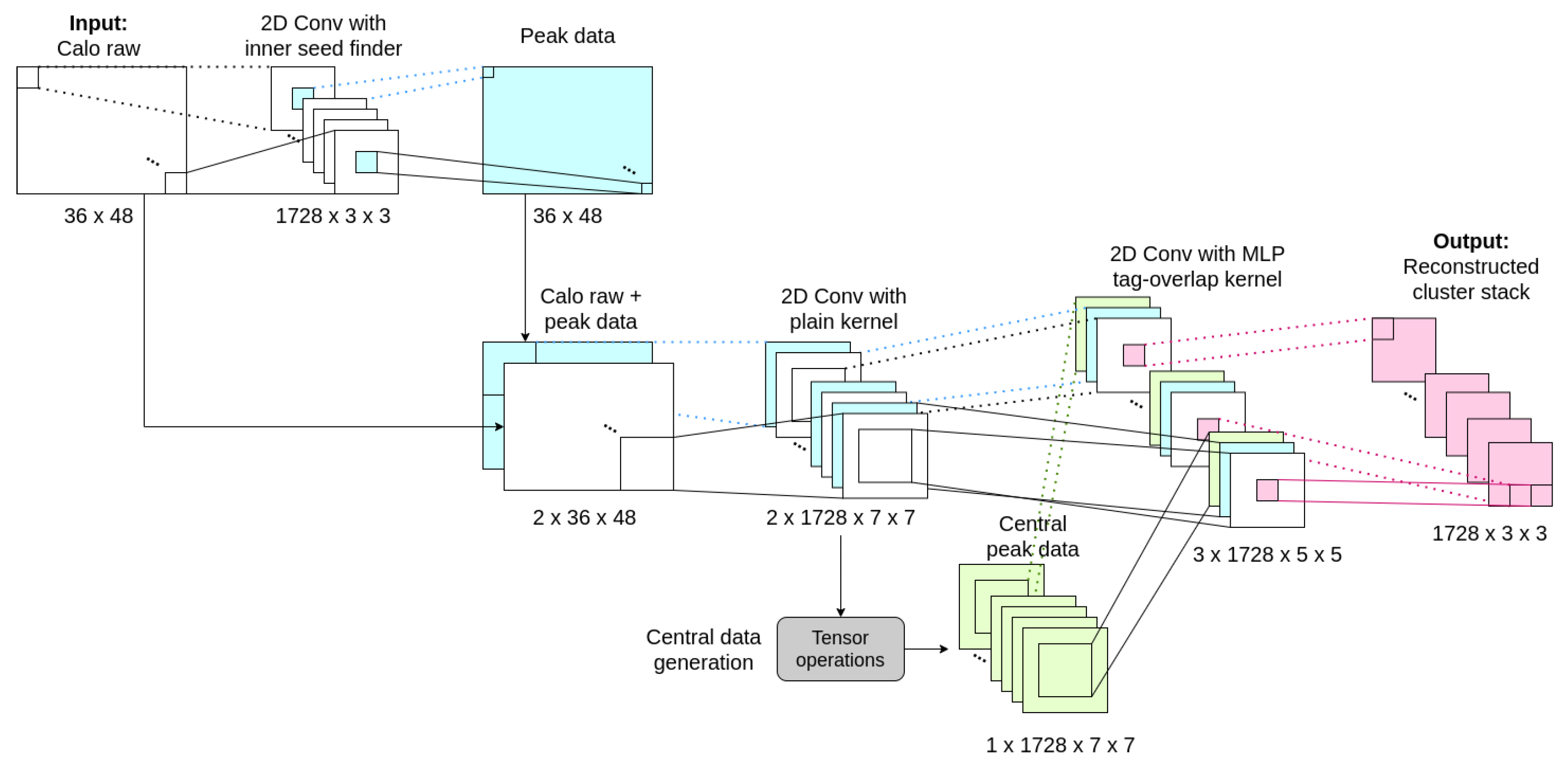
3.4. Clustering and Overlap Formulation

For the case of the last step of the reconstruction, the overlap algorithm needs to resolve the cases where a cell belongs to more than one cluster. To do so, the energy of that cell needs to be distributed among the involved clusters, depending on the total energy of each cluster. To be specific, since the energy measured in an overlapping cell may come from the addition of two different particles, one fraction of the overlapping cell energy belongs to one particle and the rest of the fraction to the other particle. Therefore, the desired output for this step is, given an input cell with overlap, the part of the energy designated to each of its contributing clusters. In case the cell does not have overlap, the output needs to be the same energy value of the input.
To correctly perform the distribution of the energy in case of overlap, the algorithm needed to know which cluster is the fraction of energy going to belong. Since there is a maximum of four possible clusters contributing to a cell by construction (see Figure 3), each fraction operation needs to be related to one of the clusters involved in the overlap. Two conclusions can be extracted at this point for the overlap cases:
  • The neighborhood window for this step needs to be big enough to identify all the cells belonging to the possible clusters causing overlap. This number corresponds with 24 neighbors inside a 5 × 5 square window around the given cell, as can be seen in Figure 3.
  • Extra information needs to be added to the 5 × 5 window, indicating the cluster to which the energy fraction is going to be part of. Since each fraction of energy needs to be assigned to a certain cluster, in the overlap cases, the same 5 × 5 window must be evaluated as many times as the number of clusters involved, but each time selecting a cluster that the fraction is going to contribute. This dominant cluster, within a 5 × 5 window, will be called central cluster.
In order to provide the central cluster information, before transforming the input image into blocks of 5 × 5 windows, there is a first transformation into windows of 7 × 7 . Within this 7 × 7 window, we can identify if the cell located at the centre is a local maximum and generates another stream of data to indicate that, for this particular window, the central cluster is the one in the middle of the window. An example representation can be seen in Figure 3 where the blue cross represents a local maxima and in this case would be marked as a central cluster as well. Regarding the identification of the central cluster, these data are generated with a masking of the local maxima stream of each 7 × 7 window. Where the mask is a 7 × 7 matrix of zeros and a single one on the central position where we expect to find the central cluster.
Once we include this third stream of information in a window of 7 × 7 , we can sub-sample all nine possible 5 × 5 windows that can fit inside the 7 × 7 . At this time, we have, on a single 5 × 5 sample, the data regarding the readout cells of the calorimeter, the local maxima information and the central cluster information. It is prepared to generate a prediction of the designated energy partition of the cell located at the centre of the window concerning the central cluster.
Gathering the previous concepts, the cellular automaton formulation of this step has the following characteristics:
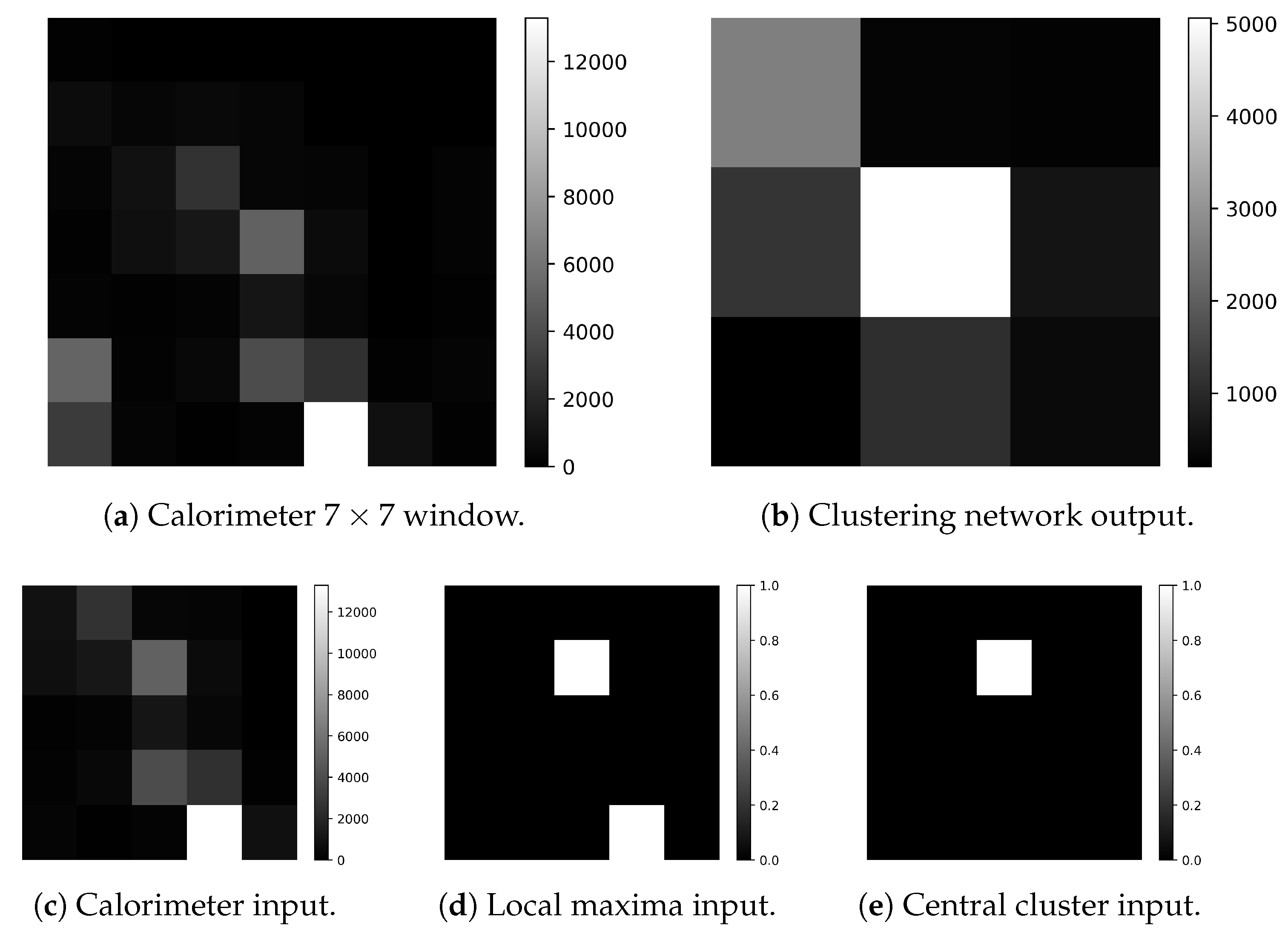
  • States: 10,240. Since the algorithm needs to give, as output, a value concerning the energy of a cell, the CA must have enough states to model the full calorimeter sensitivity, which is of 12 bits on the ADC lecture with a gain of 2.5 MeVs per ADC value ( 2 12 × 2.5 ).
  • Neighborhood: 24 cells. As explained above, the window around a cell to predict its value needs to be of 5 × 5 cells.
  • Ruleset function: at this point of the reconstruction, we have three streams of information:
    Original data sample. Obtained from the calorimeter simulation with values from 0 to 10,240.
    Local maxima information. Obtained from the output of the local maxima finder network. With values from 0 to 1.
    Central cluster information. Obtained from the masking of the central cell on each 7 × 7 window from the image. With values from 0 to 1.
    At this point, the ruleset function for this step defines the fractioning of a cell’s energy in case of overlap in Equation (3). In the same equation, num_clusters refers to the number of local maxima that could be causing overlap. As an example, if we look at the purple circle in Figure 3 to account for num_clusters, the positions marked with a purple X should be checked.
c i , j t + 1 = c i , j t C 0 k = 0 K C k , for K = n u m _ c l u s t e r s if K > 1 c i , j t , otherwise ,
where
C k = m = 1 1 n = 1 1 c o + m , p + n t
and variables o and p stand for the local maxima coordinates of cluster k in the 5 × 5 image. For k = 0 the cluster is specifically the marked as central cluster, the one in the center of the 7 × 7 window.
Before starting with the network training, there is a key aspect on the ruleset function that affects the learning capacity of a convolutional network, like the ones used on the first step. It can be seen that, for the second condition, there is a division that transforms the function into a non-linear behavior. Following the universal approximation theorem [18], there needs to be at least one hidden layer to approximate non-linear functions. However, the previous used convolutional architectures had in fact two and three hidden layers, yet the convolutional layer itself does not have a hidden layer structure on the convolution operation. The convolution is performed through the multiplication between the data and a linear kernel of parametric values; hence, there is no chance for this convolution to be able to learn the desired non-linear behavior before losing the neighborhood information on the dense layers. Therefore, the strategy for the network architecture is to use a multilayer perceptron (MLP) structure and train it to be the kernel of the convolution.
Following this strategy, one MLP network is enough for the three regions, since the sampling into 5 × 5 windows normalizes the input beyond the different region granularity. In this case, the network architecture consists of four dense layers and the output layer is a single neuron representing the predicted value of the central input cell. Hence, the network will be trained as a regressor. The output values need to be aggregated in groups of nine concerning the predicted values from a cluster at all cells of the calorimeter. As an example of the data used for the training of this network, see Figure 4.
Regarding the training dataset generation, the same numerical value independence from the first formulation is observed in this ruleset function. However, in this case, the conditions of the function are not so simple to achieve in a homogeneous scenario using randomly generated samples. At this point, we decided to take a set of only 2000 samples of LHCb simulation data and take a selected subset of approximately 30,000 windows of 7 × 7 centered on a cluster. The selection has taken into account the balancing of the dataset between six different cases specified in Table 2. Case 6 was included to enhance the training of the fraction operation when clusters have a big energy difference between them because on these cases big clusters tend to mask completely smaller clusters on its surroundings. Since case 5 has the lowest number of samples, we chose to increase its samples rotating each window by 90 , 180 and 270 , reaching more than 5000 different samples for that case. Finally, the balanced dataset was constructed, collecting 5000 samples from each of the six cases and subsampling nine windows of 5 × 5 for each of them, reaching a combined number of 270,000 samples for the training.
As it can be seen in Table 2, there is an RMSE value for each datum case. This gives an overview of the precision of the network as a function of the data complexity. Since case 1 stands for samples in which there are no clusters around, it is expected to have the lowest RMSE value. Once the samples start increasing in number of clusters involved, the RMSE value goes up accordingly. It is also expected to observe an increase in the error with the increment on data complexity. A good “symptom” is to see the case 6 samples, which have increased complexity regarding the energy difference between clusters, showing to have good performance. Even though the RMSE values are considerably low inside the full calorimeter range, it must be stated that the average energy value seen in the dataset used is of 1202.64 MeVs. With respect to that value, the maximum RMSE obtained from group 5 represents 20.3 % . However, it must be taken into account that the RMSE metric is sensitive to out layers.
A summary of the network parameters for this reconstruction step is provided in Table 3. Given the regressive nature of this network, results, in terms of training performance, are measured with the RMSE metric, comparing all the values predicted by the network to the results of applying the CA rules to the training input samples. Considering the reference of the mean energy value seen in the training samples, the RMSE of the network represents 14 % of the average energy.
Aiming to provide a detailed overview of the structured proposal, gathering the relations between the neural networks and the data, Figure 5 shows the entire dataflow of the reconstruction process for the inner calorimeter region. The diagram starts with the list of energy cells transformed into an image and ends with the list of reconstructed clusters. For the other two regions, the structure is maintained, but the shapes of the constructed images adapt to each region size.

4. Results

The results provided in this paper were obtained operating on a computer with the following properties: memory of 15.5 GB, processor Intel Core i7-6500U CPU @ 2.50 GHz × 4 , disk capacity of 512.1 GB with Ubuntu 20.04.1 LTS 64-bit OS. The algorithms are coded in Python 3.8 and the explained neural networks have been built and trained using the TensorFlow 2.3.0 library.
Aiming to make a fair comparison, in terms of computational performance between the proposed reconstruction algorithm and the original implementation of LHCb in a local environment, a version of the original calorimeter reconstruction implemented in LHCb was replicated in Python with the same computational complexity, referred to as the Python version of LHCb algorithm.
To make sure the comparison between both algorithms was fair, we defined a metric of efficiency on the reconstruction as relative error. This relative error calculated the difference of energy between reconstructed clusters and the true clusters reconstructed by the original LHCb reconstruction algorithm implemented in the LHCb framework. Using the relative error metric in the reconstructed clusters from the proposed deep learning algorithm gives as a result the first entry in Table 4. In the same table, we find the relative error for the reconstructed clusters obtained with the Python version of the LHCb algorithm. The values shown, concerning the two compared algorithms in relative error, were obtained as the mean values from over 200 simulation samples from the full LHCb calorimeter. It can be observed that the proposed deep learning approach shows, in general, a lower relative error value than the original version. Although this needs to be studied in detail with further experimentation, these results give us a hint that the two algorithms behave as expected and further comparisons will be fair.
Results, in terms of computational performance, are measured as the time in seconds elapsed between the reading of the readout cell values, and the generation of the list of clusters for the three regions of the calorimeter. The execution of both methods was done using a single thread in each case. Figure 6 shows a plot of the computational time for the number of energy cells (hits) on a single sample of a calorimeter simulation (event). The time plotted is measured as a mean of one hundred iterations on the same event for 200 different events. Looking at the curve from the Python version of the LHCb algorithm (iterative), it performs really fast in events with a low number of energy cells. However, it shows a clear quadratic growth with the number of cells activated. On the other hand, the deep learning approach (DL total) shows nearly constant behavior towards the number of cells. Although it has a small positive slope of 4.97 × 10 6 , the tendency shows to be linear. Even so, around 72 % of the events processed in the testing have less than 2575 energy cells and, therefore, stay under the time performance curve of the deep learning approach. Even so, we achieved a constant computational time with independence of the event complexity.
In addition, as stated in Section 3.2, for the first step of the proposed reconstruction process, the information from the three regions of the calorimeter needs to be treated separately. Given that the reconstruction process is the same for each region, excepting the ad-hoc local maxima neural network, another way of accelerating the execution time is executing the reconstruction of the three regions in parallel. To approximate the behavior of such execution, Figure 6 shows the execution time measured by each of the three region reconstructions independently (DL inner, DL middle, and DL outer). It is observed that, in this parallel condition, the maximum time is achieved by the outer reconstruction, since it has the highest number of readout cells. Although more studies should be made in this direction, the proposed deep learning algorithm shows that it benefits from a parallel execution.

5. Discussion

Within the development of this proposal, there are several things that have been learned. We have seen that, for the specific problem of calorimeter reconstruction in LHCb, segmenting the reconstruction steps can help in simplifying the development of a deep learning solution. Moreover, as seen in Section 3.2, data can be artificially generated as long as they correctly equally represent all cases to be learned. For more complex functions, such as the one seen in Section 3.4, the understanding of the rules also leads to a simplification of the dataset, where we were able to extract thousands of samples from only 2000 full LHCb simulated events. Understanding that there is no need to work with full simulation data to train specific networks can simplify the training dataset generation on further deep learning developments for the calorimeter reconstruction. In other words, we trained neural networks on the rules that solve a general formulation of the problem. It was proven that the network learns the application of the formulated rules in a generalized context. The complexity reduction on the training data was also reflected into a fast training process and the simplification of the networks, in terms of architecture and the number of parameters, compared with previous deep learning approaches.
Comparing the results with the state-of-the-art, we improved the relation between the network’s complexity and the amount of training data. Furthermore, the proposed model is validated by construction, since the same reconstruction steps as the current method are being reproduced.
As a proof of concept, the performance comparison in this paper is done with the current implementation of the reconstruction self-implemented in Python. In terms of computational time, there is a clear gain in the reconstruction complexity with the proposed approach. However, the execution time could possibly be reduced with a vectorized implementation of the proposal. Apart from that, the proposed implementation clearly benefits from parallel execution, reducing the computational time by nearly a factor three. Moreover, its convolutional formulation could benefit even more from a GPU architecture without conditioning the efficiency, as the insight neural networks and convolutional operators are highly parallelizable.
Despite the results, there is still room for improvement in terms of performance. Due to the region-independent strategy used in this approach; clusters that fall in the boundary regions of the calorimeter are now reconstructed partially as two separate clusters in each region. There is the idea of using a graph neural network (GNN) with similar training as the MLP, in order to perform the reconstruction in the boundary regions, as GNNs can model irregular neighborhoods. Another aspect that needs to be worked is the identification of π 0 particles. By nature, the two photons of the decay of energetic π 0 particles arrive at the calorimeter as two very close similar energy particles, but need to be reconstructed as a single cluster. Hence, the window that surrounds a pair of photons is bigger than the defined 3 × 3 . With the current training of the MLP in our proposal, the network wrongly reconstructs these specific photons as two very close overlapping clusters. There is the idea of improving this shortcoming, re-training the network of the current implementation to identify the defined photons and make an ad-hoc reconstruction for those cases.
In conclusion, we implemented and tested an alternative approach to the LHCb calorimeter reconstruction. It adapts the current reconstruction steps to a formulation that can be learned by simple deep learning structures. With this, we make sure that the reconstruction process is correct as it mimics the implementation of the current algorithm, gaining in computational complexity. Results from the testing show interesting behavior, in terms of computational time, which could be promising for a full calorimeter reconstruction implementation on GPUs.

Author Contributions

Conceptualization, N.V.C., M.C.G., E.G.R. and X.V.-C.; methodology, N.V.C., M.C.G., E.G.R. and X.V.-C.; software, N.V.C.; validation, N.V.C., M.C.G., E.G.R. and X.V.-C.; formal analysis, N.V.C., M.C.G., E.G.R. and X.V.-C.; investigation, N.V.C., M.C.G., E.G.R. and X.V.-C.; resources, N.V.C., M.C.G., E.G.R. and X.V.-C.; data curation, N.V.C., M.C.G., E.G.R. and X.V.-C.; writing—original draft preparation, N.V.C., M.C.G., E.G.R. and X.V.-C.; writing—review and editing, N.V.C., M.C.G., E.G.R. and X.V.-C.; visualization, N.V.C., M.C.G., E.G.R. and X.V.-C.; supervision, M.C.G., E.G.R. and X.V.-C.; project administration, M.C.G., E.G.R. and X.V.-C.; funding acquisition, M.C.G., E.G.R. and X.V.-C. All authors have read and agreed to the published version of the manuscript.

Funding

This research was funded by Ministerio de Ciencia e Innovación grant number PID2019-106448GB-C32.

Institutional Review Board Statement

Not applicable.

Informed Consent Statement

Not applicable.

Data Availability Statement

No new data were created or analyzed in this study. Data sharing is not applicable to this article.

Conflicts of Interest

The authors declare no conflict of interest.

References

  1. Alves, A.A., Jr.; Andrade Filho, L.; Barbosa, A.; Bediaga, I.; Cernicchiaro, G.; Guerrer, G.; Lima, H., Jr.; Machado, A.; Magnin, J.; Marujo, F.; et al. The LHCb detector at the LHC. J. Instrum. 2008, 3, S08005. [Google Scholar]
  2. Evans, L.; Bryant, P. LHC Machine. JINST 2008, 3, S08001. [Google Scholar] [CrossRef] [Green Version]
  3. Bediaga, I.; Torres, M.C.; De Miranda, J.; Gomes, A.; Massafferri, A.; Rodriguez, J.M.; dos Reis, A.; Aoude, R.; Amato, S.; Akiba, K.C.; et al. Physics case for an LHCb Upgrade II-Opportunities in flavour physics, and beyond, in the HL-LHC era. arXiv 2018, arXiv:1808.08865. [Google Scholar]
  4. LHCb Collaboration. Throughput and Resource Usage of the LHCb Upgrade HLT; Technical Report; LHCB-FIGURE-2020-007; CERN: Geneva, Switzerland, 2020. [Google Scholar]
  5. Omelaenko, O.; Dalpiaz, P.; Guzik, Z.; Spiridenkov, E.; Jarron, P.; Semenov, V.; Ocariz, J.; Khan, A.; Perret, P.; Schneider, O.; et al. LHCb Calorimeters: Technical Design Report; Technical Report; LHCb-TDR-002; CERN: Geneva, Switzerland, 2000. [Google Scholar]
  6. Breton, V.; Brun, N.; Perret, P. A Clustering Algorithm for the LHCb Electromagnetic Calorimeter Using a Cellular Automaton; Technical Report; CERN-LHCb-2001-123; CERN: Geneva, Switzerland, 2001. [Google Scholar]
  7. Breton, V.; Fonvieille, H.; Grenier, P.; Guicheney, C.; Jousset, J.; Roblin, Y.; Tamin, F. Application of neural networks and cellular automata to interpretation of calorimeter data. Nucl. Instrum. Methods Phys. Res. Sect. A Accel. Spectrometers Detect. Assoc. Equip. 1995, 362, 478–486. [Google Scholar] [CrossRef]
  8. Casolino, M.; Picozza, P. A cellular automaton to filter events in a high energy physics discrete calorimeter. Nucl. Instrum. Methods Phys. Res. Sect. A Accel. Spectrometers Detect. Assoc. Equip. 1995, 364, 516–523. [Google Scholar] [CrossRef] [Green Version]
  9. Denby, B. Neural networks and cellular automata in experimental high energy physics. Comput. Phys. Commun. 1988, 49, 429–448. [Google Scholar] [CrossRef]
  10. Baldanza, C.; Bisi, F.; Bruschi, M.; D’Antone, I.; Meneghini, S.; Rizzi, M.; Zuffa, M. A cellular neural network for peak finding in high-energy physics. In Proceedings of the 2000 6th IEEE International Workshop on Cellular Neural Networks and their Applications (CNNA 2000) (Cat. No. 00TH8509), Catania, Italy, 25 May 2000; pp. 443–448. [Google Scholar]
  11. Mazurek, M. Deep Learning Solutions for 2D Calorimetric Cluster Reconstruction at LHCb. In Proceedings of the 4th Inter-Experiment Machine Learning Workshop, Zürich, Switzerland, 19–23 October 2020. [Google Scholar]
  12. Redmon, J.; Farhadi, A. Yolov3: An incremental improvement. arXiv 2018, arXiv:1804.02767. [Google Scholar]
  13. Canudas, N.V.; Cardona, X.V.; Gómez, M.C.; Ribé, E.G. Deep Learning approach to LHCb Calorimeter reconstruction using a Cellular Automaton. EPJ Web Conf. EDP Sci. 2021, 251, 04008. [Google Scholar] [CrossRef]
  14. Abba, A.; Caponio, F.; Cusimano, A.; Geraci, A.; LHCb Collaboration. LHCb Particle Identification Upgrade: Technical Design Report; CERN: Geneva, Switzerland, 2013. [Google Scholar]
  15. Bediaga, I.; Chanal, H.; Hopchev, P.; Cadeddu, S.; Stoica, S.; Calvo Gomez, M.; T’Jampens, S.; Machikhiliyan, I.V.; Guzik, Z.; Alves, A.A., Jr.; et al. Framework TDR for the LHCb Upgrade: Technical Design Report; Technical Report; LHCb-TDR-012; CERN: Geneva, Switzerland, 2012. [Google Scholar]
  16. Neumann, J.; Burks, A.W. Theory of Self-Reproducing Automata; University of Illinois Press: Urbana, IL, USA, 1966; Volume 1102024. [Google Scholar]
  17. Gilpin, W. Cellular automata as convolutional neural networks. Phys. Rev. E 2019, 100, 032402. [Google Scholar] [CrossRef] [PubMed] [Green Version]
  18. Cybenko, G. Approximation by superpositions of a sigmoidal function. Math. Control. Signals Syst. 1989, 2, 303–314. [Google Scholar] [CrossRef]
Figure 1. The electromagnetic calorimeter 3d-view from behind the detector towards the interaction point [5].
Applsci 11 11467 g001
Figure 2. Samples of the data used for the training and testing of the local maxima finder network for the inner region of the LHCb calorimeter. The training input sample (a) is artificially generated and the output sample for training (b) is obtained applying the CA rules on the (a) sample. The testing input sample (c) is an LHCb simulation and the testing output sample (d) again generated applying the CA rules on sample (c) and represent the expected output from the network. Then image (e) is the real output obtained from the network trained to reproduce the CA when sample (c) is on the input, and is compared to sample (d) to obtain the accuracy value.
Applsci 11 11467 g002
Figure 3. Diagram representing the possible cluster centre positions overlapping with the central cluster in a 7 × 7 window. The maxima positions are marked with crosses and the two overlap cells that need to be predicted are marked with a circle.
Applsci 11 11467 g003
Figure 4. Samples of the data used for the training of the clustering and overlap network. The three streams of data (ce) are extracted from the analysis of a 7 × 7 window (a). Image (b) shows the output predicted by the network representing the reconstructed cluster located at the centre of the (a) sample.
Applsci 11 11467 g004
Figure 5. Detailed scheme of the proposed reconstruction dataflow for the inner calorimeter region.
Applsci 11 11467 g005
Figure 6. Scatter plot of the mean computational time over the number of readout cells per event from LHCb simulations. Comparing the Python version of the LHCb algorithm (iterative) and the proposed deep learning implementation (DL total) with executions segmented by regions (DL inner, DL middle, DL outer). Hits refer to the readout cells with energy on a sample.
Applsci 11 11467 g006
Table 1. Parameter summary of the local maxima finder neural networks.
Region Image
Shape
Training
Samples
Neurons
Per Layer
ParametersTraining
Time
Accuracy
Outer 64 × 52 10,000[20, 20, 20, 10, 2]12721354.7 s99.96%
Middle 64 × 40 10,000[20, 20, 20, 10, 2]12721052.3 s99.92%
Inner 48 × 36 10,000[10, 10, 10, 2]342461.8 s99.93%
Table 2. Case characteristics in the balanced dataset for the MLP training. Case 6 is a selection of samples with overlap with at least one cluster, but where the energy difference between clusters is bigger than an order of magnitude. The RMSE values were extracted, comparing the network predicted values and the samples generated with the application of the CA rule.
CaseNumber of
Clusters (K)
Overlap with
Central Cell
Samples on
2k Events
RMSE
10No153,51996.281
21No121,316135.616
32Yes (1 cluster)45,066147.501
43Yes (2 clusters)9937199.644
54+Yes (3+ clusters)1367244.312
6>1Yes (energy difference of 1 order of magnitude)6816181.693
Table 3. Parameter summary of the cluster and overlap neural network.
Region Image
Shape
Training
Samples
Neurons
Per Layer
ParametersTraining
Time
RMSE
All 5 × 5 270,000[64, 64, 64, 32]108,9932130.4 s168.884
Table 4. Results concerning the mean value and standard deviation of the relative error measured as the difference of energy reconstructed per cluster from a total of 200 simulated events.
Algorithms Mean of
Relative Error
STD of
Relative Error
Deep Learning0.0560.105
Python version of LHCb algorithm0.0790.159
Publisher’s Note: MDPI stays neutral with regard to jurisdictional claims in published maps and institutional affiliations.

