Study on the Influence of Triangular Groove Structure on Steady-State Flow Force Compensation Characteristics

Abstract

In this study, a structurally improved spool was designed. The diameter of one side of the spool stem was reduced, making the spool stem into a rounded table shape. A triangular groove was circumscribed on the step and on the same side. After liquid flow was guided through the triangular groove, the flow direction changed. A flow component in the negative direction was generated, which reversely impacted the liquid flow in the positive direction. The liquid flow angle at the outlet increased; that is, jet angle increased and flow force decreased. The simulation results show that, increasing the depth, H, of the triangular groove has a positive effect on flow-force compensation and was conducive to the stability of the valve core. Properly increasing the groove’s bottom diameter, D₁, of the triangular groove was conducive to the stability of the spool, but when D₁ was too large, the flow force increased. The experimental results are consistent with the simulation results, which proves that the improved structure can effectively reduce the flow force of the spool.

1. Introduction

Hydraulic technology is widely used in modern industry because of its remarkable characteristics of large power–weight ratio, high control accuracy and good stability [1,2]. The design and optimization of hydraulic components is an important link in improving hydraulic technology [3,4]. A hydraulic control element is one of the basic components of a hydraulic system. It mainly refers to hydraulic control valves, including pressure valves, flow valves and direction valves, though slide and pilot valves are commonly used. The working principle is to control the flow and flow direction of fluid through the relative movement of the valve core and the valve body, and directly or indirectly controlling the movement of an actuator [5]. As important parts of a hydraulic system, the static and dynamic characteristics of hydraulic valves have an important impact on the stability of a hydraulic system [6,7]. In recent years, flow force has become a research hotspot of scholars the world over. Flow force is divided into transient flow force and steady-state flow force, in which steady-state flow force has a great influence on the static characteristics of hydraulic valves. As early as the 1950s, Lee and Blackburn [8] researched steady-state flow forces. Amirante et al. [9,10] analyzed the driving forces on a 4/3 hydraulic open center directional control valve. The valve was tested with different pump flow rates, as well as with different pressure drops. Their results showed important differences between an open-center valve and a closed-center one. Rannow and Li [11] proposed a soft switching approach to eliminate the majority of valves’ transition losses. The simulation results showed that the soft switching approach has the potential to improve the efficiency of on/off-controlled systems. They studied the hydrodynamics of a hydraulic valve based on one-dimensional and three-dimensional CFD modeling methods to analyze the flow-force, pressure and velocity characteristics of hydraulic valve. Ye et al. [12] clarified the effects of a grooved shape on flow characteristics through computational fluid dynamics (CFD) and experimental investigations. They furthermore analyzed the changes of restricted locations along with the openings to calculate the flow areas of the notches. The discharge coefficient, as a function of groove geometry, flow condition, fitting coefficients and its stable value, was deduced, proving to be quite consistent in their experimental result. Lu [13,14] researched the effects of radial flow force and static pressure upon the lateral force. The jet angle was discovered not only to be related to the annular orifice opening and gap clearance but was also influenced by the flow direction and control-surface profile.

Lü et al. [15] applied a numerical simulation method based on the flow-solid interaction (FSI) to observe the variation of the jet force when the flapper is moving. They established the relationship between the movement of the flapper, the flow field distribution, the jet force and the inlet pressure. Lu et al. [16] the stability of two-dimensional (2D) servo valve and its influencing factors and concluded that the steady-state flow force generated by fluid flowing through the spiral valve port belongs to space force which is not conducive to the stability of the valve core. Wang et al. [17] established the dynamics characteristics of a poppet relief valve containing both a transient flow force and a steady flow force. They observed that the flow force had an important impact on the stability of the valve. Qu et al. [18] built a mathematical flow-force model of converged flow valves and studied the influences of different fit clearances on the steady-state flow forces of valves. The results showed that the fit clearance had an important influence on valves’ steady-state flow force. Zhang et al. [19] established a three-dimensional model of computational fluid dynamics by using CFD-ACE + software. The instantaneous flow field, spool displacement, flow force and deformation of the hydraulic control directional valve with three throttling structures were compared. The above literature shows that flow force has an important impact on the stability of hydraulic valves. In order to ensure the operability and accuracy of hydraulic valve, flow force must be compensated. Herakovic et al. [20] defined the structure of a slide spool and a spool sleeve in detail and used CFD simulation calculation to reduce the steady-state flow force by changing the geometry of the spool sleeve and spool. Altare et al. [21] studied the 3D and 0D simulation of a conical popped pressure-relief valve with flow-force compensation and created a dynamic model. The model was able to determine the equilibrium position of the poppet in order to estimate the regulated pressure as function of the flow rate. They also studied influence of the deflector geometry on the opening force to realize the compensation of flow force. Tan et al. [22] proposed a method aimed at reducing the steady-state axial flow force working on the main spool of a diverged flow cartridge proportional valve; they found a rule governing how these parameters influence flow force by a series of computational fluid dynamics (CFD) simulations. Roberto and Massimo [23] studied the effect of poppet geometry on the flow-pressure characteristics of a direct-acting pressure-relief valve. A dynamic 3D-CFD model was built in ANSYS Fluent to predict the flow-pressure characteristics of the valve for different spring preload settings and deflector geometries. Then, they calculated the effect of the geometric parameters of the poppet and optimized the cone angle and the position of the deflector to compensate for the flow force. Zhang and Li [24] proposed machining an annular groove on a spool core to compensate for flow force, and analyzed the influence of the depth of the spool sleeve’s sunk groove, the depth and width of the annular groove of the spool core and other factors of its compensation characteristics. Dong and Fu [25] used the Fluent simulation software to explore the effects of groove depth and included angle of the throttling groove and the deflection the angle between the V-groove and the symmetrical plane of the spool sleeve on the steady-state flow force acting on the spool, as well as the flow characteristics of the spool port.

In this paper, the flow force of a hydraulic valve is analyzed, and an improved method of spooling is proposed. Based on the force and jet angle of the spool, the influence law of the structural parameters of the improved spool on flow-force compensation characteristics is further studied through simulation, and an experimental platform is built to verify the simulation results.

2. Flow Force Analysis

Figure 1 shows the stress on the spool, and the flow force can be expressed as follows:

$$F_F=F_{{\tau }_{rod}}+F_s+F_d$$

(1)

where $F_F$ is flow force. $F_{{\tau }_{rod}}$ is the viscous force generated by fluid acting on the spool. $F_s$ is the static force generated by fluid acting on the spool. $F_d$ is the dynamic force generated by fluid acting on the spool.

Selecting ‘right’ as the positive direction, $F_{{\tau }_{rod}}$, $F_s$ and $F_d$ can be expressed as follows:

$$F_{{\tau }_{rod}}={\displaystyle {\iint }_{A_{rod}}{\tau }_{rod}dA}$$

(2)

$$F_s={\displaystyle {\iint }_{A_r}{p}_{s2}dA}-{\displaystyle {\iint }_{A_l}{p}_{s1}dA}$$

(3)

$$F_d={\displaystyle {\iint }_{A_r}{p}_{d2}dA}-{\displaystyle {\iint }_{A_l}{p}_{d1}dA}$$

(4)

where ${\tau }_{rod}$ is the shear force generated by fluid acting on the spool stem. $p_{s1}$ and $p_{s2}$ are the static pressure generated by fluid acting on the left shoulder surface 1 and the right shoulder surface 3 of the spool. $p_{d1}$ and $p_{d2}$ are dynamic pressure generated by the fluid acting on the left shoulder surface 1 and the right shoulder surface 3 of the spool. $A_{rod}$ is the surface area of the spool stem. $A_l$ and $A_r$ are the areas of the left shoulder surface 1 and the right shoulder surface 3 of the spool.

So, the flow force can be expressed as follows:

$$F_F={\displaystyle {\iint }_{A_{rod}}{\tau }_{rod}dA}+{\displaystyle {\iint }_{A_r}{p}_{s2}dA}-{\displaystyle {\iint }_{A_l}{p}_{s1}dA}+{\displaystyle {\iint }_{A_r}{p}_{d2}dA}-{\displaystyle {\iint }_{A_l}{p}_{d1}dA}$$

(5)

In this paper, the forces of the spool in the steady state are studied, and the transient flow force is ignored; that is, the dynamic forces generated by the fluid acting on the spool are ignored. The flow force of the spool can be expressed as follows:

$$F_F={\displaystyle {\iint }_{A_{rod}}{\tau }_{rod}dA}+{\displaystyle {\iint }_{A_r}{p}_{s2}dA}-{\displaystyle {\iint }_{A_l}{p}_{s1}dA}$$

(6)

Flow force can also be calculated by momentum theorem. Taking the fluid as the research object, the fluid is subjected to two forces: the force exerted by the spool sleeve and the force exerted by the spool. The force that the spool enacts on the fluid and the force that the fluid enacts on the spool are the action and reaction forces. Therefore, the force acting on the fluid can be expressed as follows:

$$F_{liquid}=F_{sleeve}-F_F$$

(7)

where $F_{liquid}$ is the force on the fluid. $F_{sleeve}$ is the force exerted by the sleeve on the fluid.

$F_{sleeve}$ can be expressed as follows:

$$F_{sleeve}={\displaystyle {\iint }_{A_{sleeve}}{\tau }_{sleeve}dA}\approx \alpha \mu Lq$$

(8)

where ${\tau }_{sleeve}$ is the shear force generated by the spool sleeve acting on the fluid. $A_{sleeve}$ is the contact area between the sleeve and the fluid. $\alpha$, $\mu$ and $L$ are the geometry coefficient of runner, fluid viscosity and effective length of the fluid, respectively. $q$ is flow rate.

From the momentum conservation theorem:

$$F_{liquid}=\frac{d}{dt}{\displaystyle {\iiint }_{C.V.}\rho v_{x}dV}+{\displaystyle {\iint }_{A_i}\rho v_{x}v\times idA+}{\displaystyle {\iint }_{A_o}\rho v_{x}v\times (-i)dA}$$

(9)

where $\rho$ is fluid density, $v$ is fluid velocity, $v_x$ is fluid axial velocity, $i$ is the left unit normal vector, $A_i$ is the inlet area, $A_o$ is the outlet area.

Ignoring the transient flow force, the following results can be obtained as follows:

$$F_{liquid}=\rho q{v}_2\cos {\theta }_2-\rho q{v}_1\cos {\theta }_1$$

(10)

where $v_1$ and $v_2$ are the average speeds at the inlet and outlet. ${\theta }_1$ and ${\theta }_2$ are the jet angles at the inlet and outlet. Steady-state flow force can be expressed as follows:

$$F_F=F_{sleeve}-F_{liquid}=\alpha \mu Lq+\rho q{v}_1\cos {\theta }_1-\rho q{v}_2\cos {\theta }_2$$

(11)

According to the above derivation, the steady-state flow force is in the direction of closing the valve, that is, the negative direction. The steady-state flow force value depends on the forces on the left and right shoulder of the spool and the side of the spool stem. The jet angle at the outlet also affects the steady-state flow force.

3. Modeling and Simulation

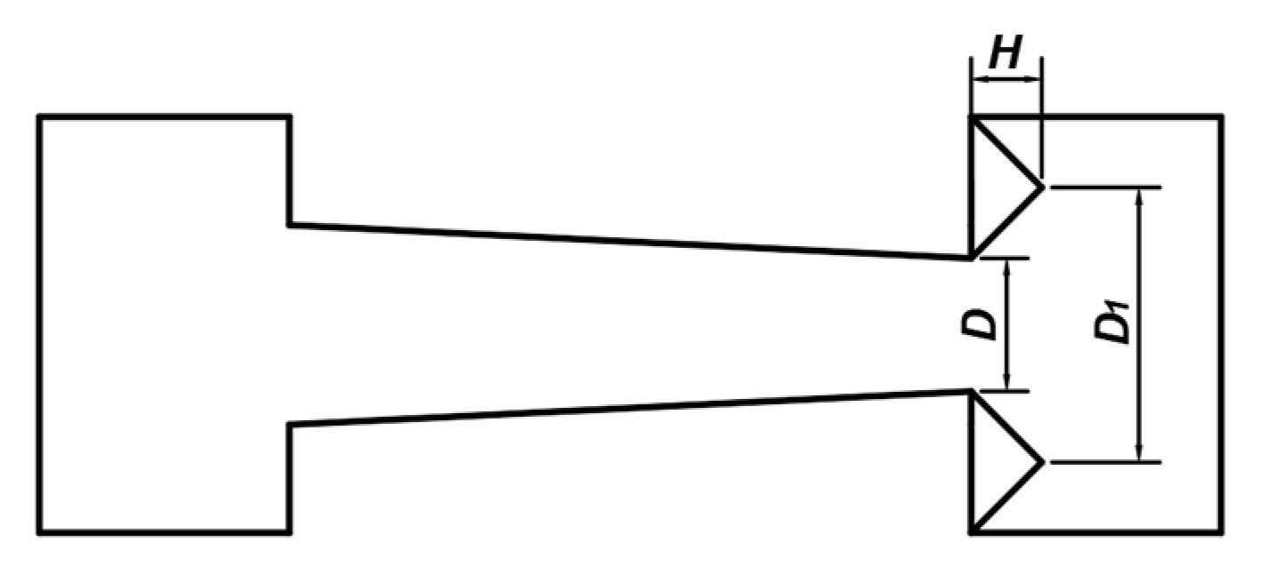
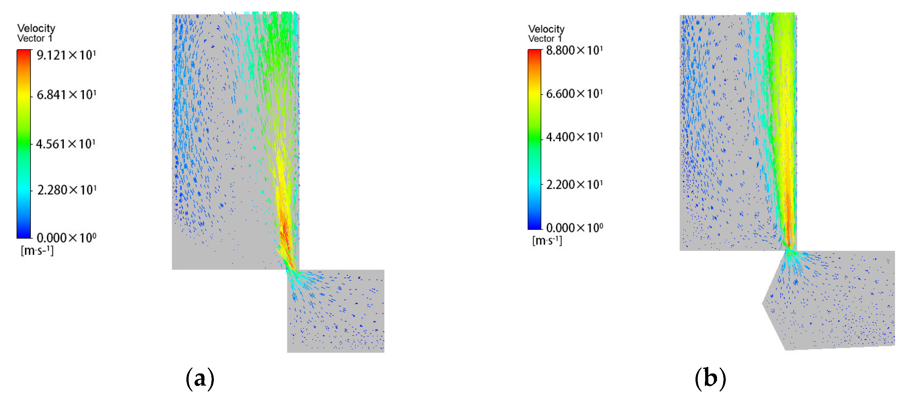
The improved spool is shown in Figure 2. In this paper, the diameter of the right spool stem is reduced on the basis of the original spool, so that the spool stem is in the shape of a round platform. A triangular groove is circumscribed on the right step, which is composed of surface 3 and surface 4. After part of the liquid flow is diverted through surface 3 and surface 4, the flow direction changes, that is, a leftward flow component is generated. This part of the liquid flow reversely impacts the liquid flow flowing to the right, which increases the jet angle at the outlet and reduces the flow force. As the diameter on the right side of the spool stem is reduced to form a round platform, the space on the right side of the spool stem is larger. This allows more fluid to flow through surface 3 and surface 4, further reducing the flow force. As shown in Figure 3, the main structural parameters of the improved spool are the right spool stem’s end diameter, D, the triangular groove’s bottom diameter, D₁, and the groove depth, H.

The three-dimensional model was established in SolidWorks and imported into ANSYS/Fluent to simulate the fluid domain. In this paper, the initial parameters are D = 8 mm, H = 4 mm, D₁ = 16 mm. The diameter of the unmodified stem is 12 mm. Reynolds number is 2351. There are three turbulence models K-ε, K-ω, and Reynolds stress in ANSYS/Fluent. K-ε model is the most widely used turbulence model in the research of hydraulic valve. Based on this model, the valve is simulated and analyzed in this paper. Turbulent kinetic energy, K, and dissipation, ε, can be derived from the migration equation, as follows:

$$\frac{\partial }{\partial \mathrm{t}}(\rho k)+\frac{\partial }{\partial x_i}(\rho k{u}_i)=\frac{\partial }{\partial x_j}[(\mu +\frac{{\mu }_t}{{\sigma }_k})\frac{\partial k}{\partial x_j}]+G_k+G_b-\rho \epsilon -Y_M+S_k$$

(12)

$$\frac{\partial }{\partial \mathrm{t}}(\rho \epsilon )+\frac{\partial }{\partial x_i}(\rho \epsilon u_i)=\frac{\partial }{\partial x_j}[(\mu +\frac{{\mu }_t}{{\sigma }_{\epsilon }})\frac{{\partial }_{\epsilon }}{\partial x_j}]+C_{1\epsilon }\frac{\epsilon }{k}(G_k+C_{3\epsilon }{G}_b)-C_{2\epsilon }\rho \frac{{\epsilon }^2}{k}+S_{\epsilon }$$

(13)

where $G_k$ is the turbulent kinetic energy generated by the average velocity gradient. $G_b$ is the turbulent kinetic energy generated by liquid buoyancy. $Y_M$ is the fluctuation expansion of the overall dissipation rate in the compressible turbulent flow. $C_{1\epsilon }$, $C_{2\epsilon }$ and $C_{3\epsilon }$ are model constants. ${\sigma }_k$ and ${\sigma }_{\epsilon }$ are the turbulent Prandtl number of $k$ and $\epsilon$, $S_k$ and $S_{\epsilon }$ are user-defined values. ${\mu }_t$ is turbulent viscosity, which can be expressed as follows:

$${\mu }_t=\rho C_{\mu }\frac{k^2}{\epsilon }$$

(14)

In this paper, the form of the pressure inlet and pressure outlet are adopted; the inlet pressure is 3 MPa and the outlet pressure is 0.5 MPa, and the fit clearance between the spool and the spool sleeve is ignored. The fluid density is 870 $\mathrm{kg}\cdot {\mathrm{m}}^{-3}$. The dynamic viscosity is 0.04 $\mathrm{kg}\cdot {\mathrm{m}}^{-1}\cdot {\mathrm{s}}^{-1}$.

4. Simulation Results and Analysis

4.1. When H and D₁ Remain Unchanged, the Influence of D Changes the Flow Force

When the fixed values H = 4 mm, D₁ = 16 mm, spool opening x_v = 1 mm are unchanged, D changes within the range of 4–12 mm, where every 2 mm is a measuring point. As shown in Figure 4, when D changes within the range of 4–12 mm, the variation range of the force on surface 1 is very small, and the maximum difference is only 0.45 N compared with the unimproved spool. The direction of the force on surface 1 is vertical surface 1 to the left. This is because the liquid flow state at the left end of the spool and the spatial distribution of surface 1 are basically not affected by the change of the diameter at the right end, and the pressure on the left side remains basically unchanged. As shown in Figure 5, as the diameter of the right end decreases, the force on surface 2 gradually increases, and the force direction is negative, that is, in the spool’s closing direction. This is because the diameters of the left and right ends of the spool are different, forming a certain stress area on the side surface of the spool stem, resulting in the leftward force. With decreasing diameter, the force on the surface 2 increases.

The forces on the improved spool surface 3 and surface 4 are shown in Figure 6. The force on the surface 3 of the improved spool increases with the decrease of diameter, D. This is because when H and D₁ remain unchanged, the smaller the D, the greater the included angle between surface 3 and the horizontal plane, and the greater the impact of liquid flow on plane 3, that is, the greater the force. At the same time, changing the diameter will not affect the spatial distribution of surface 4, and the impact of fluid on surface 4 will not change greatly, that is, the force on surface 4 is basically unchanged. As can be seen in Figure 6, the sum of the forces on surface 3 and surface 4 of the improved spool is greater than that on surface 3 of the unimproved spool, and it is in the positive direction. Although this improvement will increase the force on surface 2, the forces in the positive direction on surface 3 and surface 4 increases more. The resultant forces on surfaces 2, 3 and 4 of the improved spool are greater than those of the unimproved spool, and the direction of the resultant forces is positive. This resultant force is opposed to the flow force and can counteract part of the flow force. So, the resultant force compensates for the flow force and is conducive to the stability of the spool. The sums of forces on surfaces 1, 2, 3 and 4 of two spools are recorded in

Table 1. Sums of forces on all surfaces of the two spools.

D (mm)	Unimproved Spool	Improved Spool
4	−17.80	−5.78
6	−17.80	−5.36
8	−17.80	−5.25
10	−17.80	−5.44
12	−17.80	−5.45

.

It can be seen from Figure 7 that changing the diameter D has little effect on the jet angle. When D changes within 4–12 mm, the difference between the maximum and minimum jet angle is only 1.3°. Therefore, when changing the diameter, the flow force is mainly compensated for by the resultant forces on surfaces 2, 3 and 4. The variation of flow force with D is shown in Figure 8. With the decrease of diameter, the flow force first decreases and then increases. When D = 8 mm, the flow force is least, which is −5.25 N.

4.2. When D₁ and D Remain Unchanged, the Influence of H Change on Flow Force

When the fixed values D₁ = 16 mm, D = 8 mm, spool opening x_v = 1 mm are unchanged, H changes within a range of 2–6 mm, and every 1 mm is a measuring point. As can be seen from Figure 9, when H increases, the force on surface 1 basically remains unchanged, and the difference is only 0.59 N compared with the unimproved spool. The reason for this is the same as in the above analysis. As shown in Figure 10, since changing H does not affect the spatial distribution of surface 2, the force on surface 2 remains basically unchanged.

As H increases, the included angle between surface 3 and the horizontal plane decreases, and the impact of liquid flow on surface 3 decreases, resulting in a small increase in force on surface 3, as shown in Figure 11. As the included angle between surface 4 and the horizontal plane becomes smaller, the liquid flows to surface 4 after the diverting effect of surface 3; the impact effect on surface 4 increases, as does the force on surface 4, as shown in Figure 12. As can be seen from Figure 13, as H increases, the reverse flow angle of the liquid flowing through surface 4 increases, and the reversed, diverting effect of surface 4 increases. The liquid flowing in the negative direction reverses the liquid flowing in the positive direction, resulting in an increased jet angle at the outlet.

As shown in Figure 14, the jet angle of the improved spool is significantly larger than that of the unimproved spool. The relationship between the jet angle and H is shown in Figure 15. As the jet angle increases, the flow force decreases, and the change of flow force is shown in Figure 16.

4.3. When H and D Remain Unchanged, the Influence of D₁ Changes the Flow Force

When the fixed values H = 4 mm, D = 8 mm, spool opening x_v = 1 mm are unchanged, D₁ changes within a range of 14–22 mm, and every 2 mm is a measuring point. As can be seen from Figure 17, when D₁ becomes larger, the force on surface 1 basically remains unchanged. Compared with the unimproved spool, the difference is only 0.74 N, and the reason for this is the same as in the above analyses. Since changing D₁ does not affect the spatial distribution of surface 2, it can be seen from Figure 18 that the force on surface 2 remains basically unchanged.

With the increase of D₁, the included angle between surface 3 and the horizontal plane becomes larger, the impact of the liquid flow on surface 3 increases and the force on surface 3 increases, as shown in Figure 19. As can be seen in Figure 20 and Figure 21, with the increase of D₁, the included angle between surface 4 and the horizontal plane decreases, the force along the positive direction generated by the liquid flow impacting surface 4 decreases, the reverse diversion effect of surface 4 increases within a certain range and the jet angle also increases.

Although the force in the negative direction on surface 2 of the improved spool becomes larger, it can be seen, in Figure 19, that the sum of the forces on surface 3 and surface 4 of the improved spool is larger than that on surface 3 of the unimproved spool, both in the positive direction, and the resultant forces on surfaces 2, 3 and 4 of the improved spool are larger than those of the unimproved spool, which produces a compensatory effect. It can be seen from Figure 22 that the flow force first increases with the increase of D₁, and the minimum flow force is generated near D₁ = 18 mm, which then decreases slightly. This is because when D₁ is too large, the included angle between surface 4 and the horizontal plane is too small; the force in the positive direction generated by the liquid flow impacting surface 4 becomes smaller, and the decrease is greater than the increase of the force on surface 3. Thus, the sum of the forces on surface 3 and surface 4 becomes smaller. When the angle between surface 4 and the horizontal plane is too small, the reversed, diverting effect of surface 4 is weakened, and the jet angle increases slowly or even decreases. The relationship between jet angle and D₁ is shown in Figure 23.

5. Experimental Verification

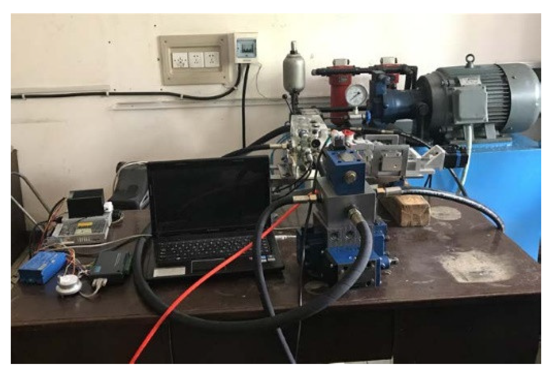
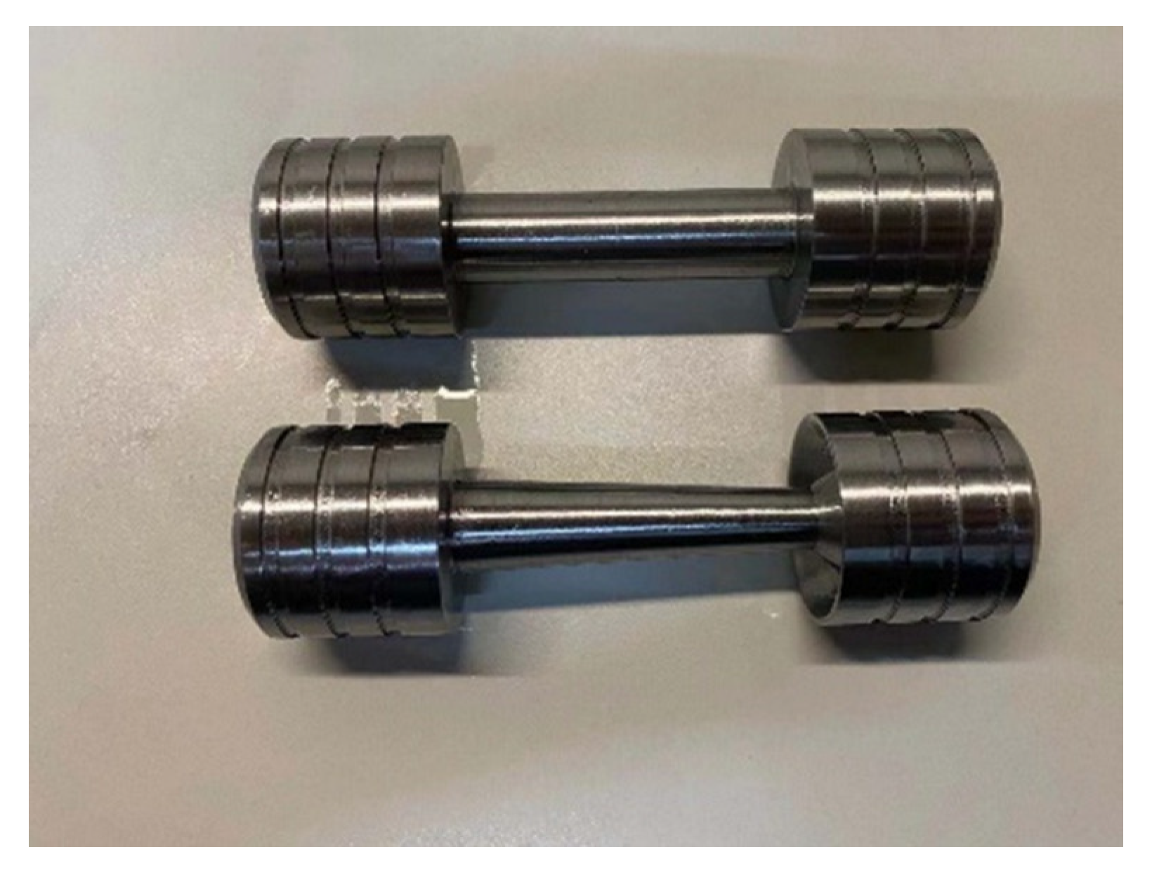
The testbed consisted of a driving device, force sensor, data acquisition card, pressure gauge, displacement sensor, solenoid valve, accumulator, relief valve, hydraulic pump and throttle valve. The hydraulic circuit is shown in Figure 24 and the testbed is shown in Figure 25. The improved spool and unimproved spool are shown in the Figure 26.

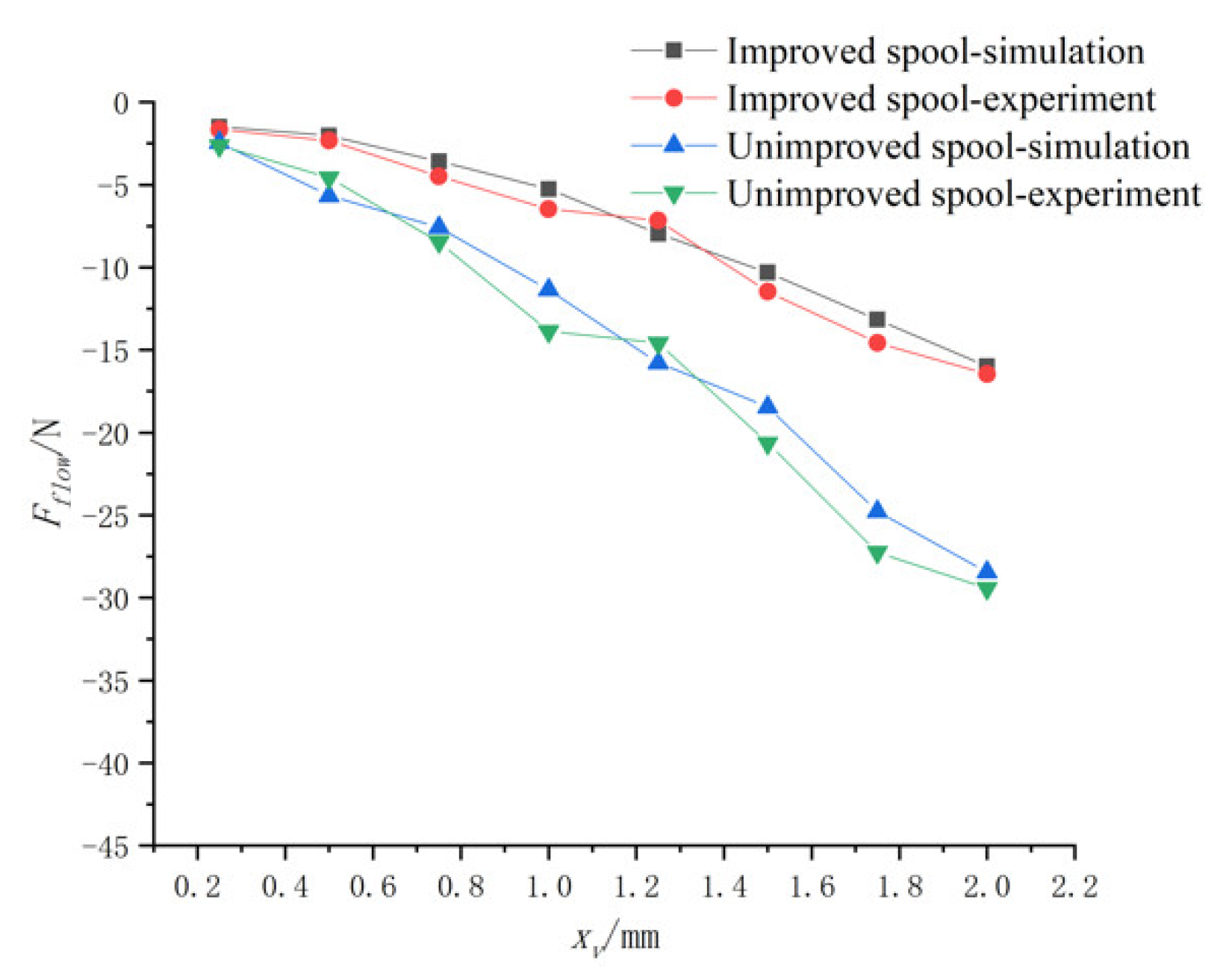
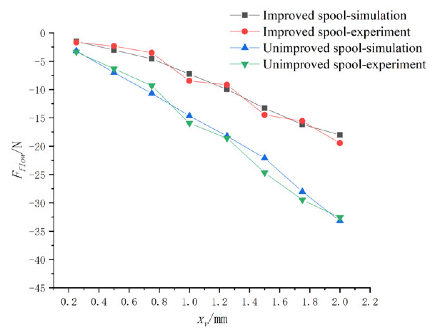
Figure 27, Figure 28 and Figure 29 show the change of flow force with the spool opening under different inlet and outlet pressure differences. The flow force increased greatly with increasing opening. Compared with the unimproved spool, the flow force of the improved spool is significantly reduced. With the increase of the opening, the decrease in flow force of the improved spool is more obvious.

In order to quantitatively study the flow-force compensation of the improved spool, the compensation coefficient $\gamma$ is defined as the flow-force increment per spool opening, and $\gamma$ can be expressed as follows:

$$\gamma =\frac{\Delta F_{flow}}{\Delta x_v}$$

(15)

Obviously, when $\gamma$ > 0, it indicates that the flow force is completely offset and produces a flow force in the opposite direction, that is, it produces over-compensation. When $\gamma$ = 0, it indicates that the flow force is completely offset. When $\gamma$ < 0, it means that part of the flow force is compensated for; and, the smaller the absolute value of $\gamma$, the more the flow force is compensated for, and the more stable is the compensation characteristic.

The flow forces under different pressure difference were fitted to the spool opening to obtain various compensation coefficients, as shown in

Table 2. Compensation coefficients.

Pressure Difference (MPa)	Unimproved Spool	Improved Spool
1.5	−6.3	−13.5
2.5	−8.9	−17.5
3.5	−12.2	−19.2

. With the increase of pressure difference, the absolute values of $\gamma$ for the two spools became larger, the compensation effect decreased, and the compensation characteristic became unstable. However, at the same pressure difference, the absolute value of the compensation coefficient of the improved spool was less than that of the unimproved spool. When the pressure difference was 1.5 MPa, the absolute value of the compensation coefficient of the improved spool was 53.3% lower than that of the unimproved spool. When the pressure difference was 3.5 MPa, the absolute value of the compensation coefficient of the improved spool was 36.5% lower than that of the unimproved spool; the compensation effect is more obvious in the case of small pressure differences.

6. Conclusions

In this paper, an improved scheme was proposed to reduce flow force. We reduced the diameter of one side of a spool stem to make shape it into a round platform. A triangular groove was circumscribed on the step of the same side, which could control the flow direction of the fluid. This increased the jet angle at the outlet and reduced the flow force. As the diameter of one side of the spool stem was reduced, the space on this side of the spool stem was also increased, such that more liquid flow could be guided through the triangular groove, further reducing the flow force.

Further, by analyzing the structural parameters of the spool, we concluded that:

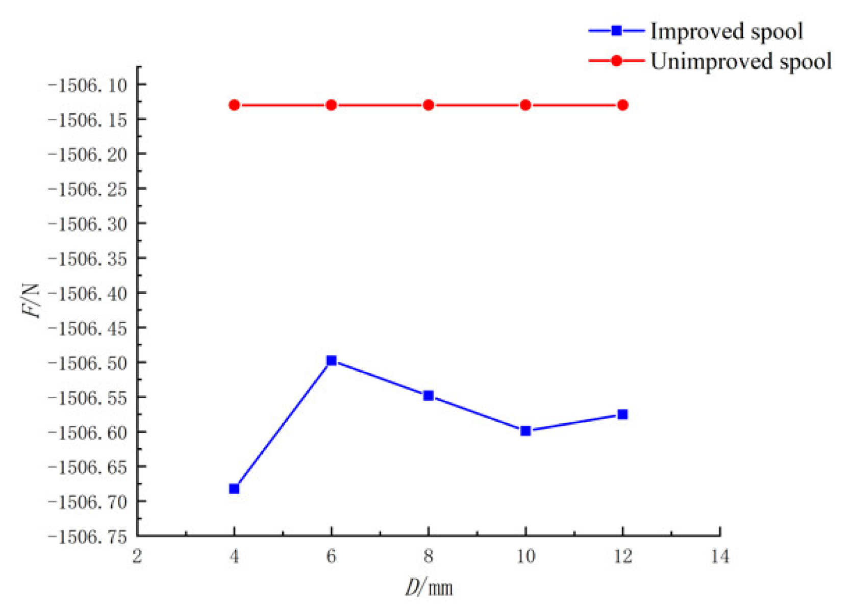
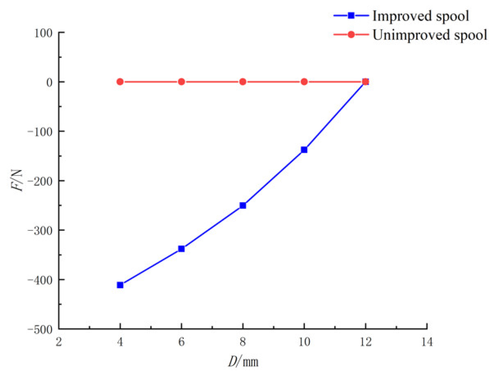
(1)

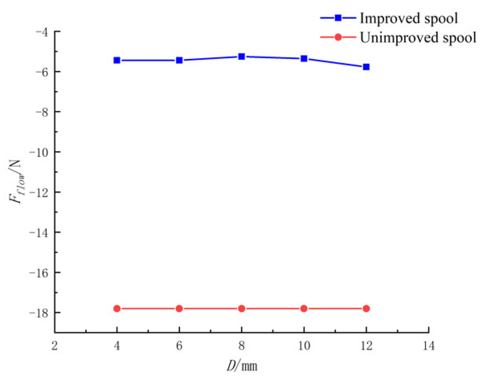
When fixed, H and D₁ remained unchanged and D became smaller, the flow force first decreased and then increased. When D = 8 mm, the flow force in the negative direction was the smallest.

(2)

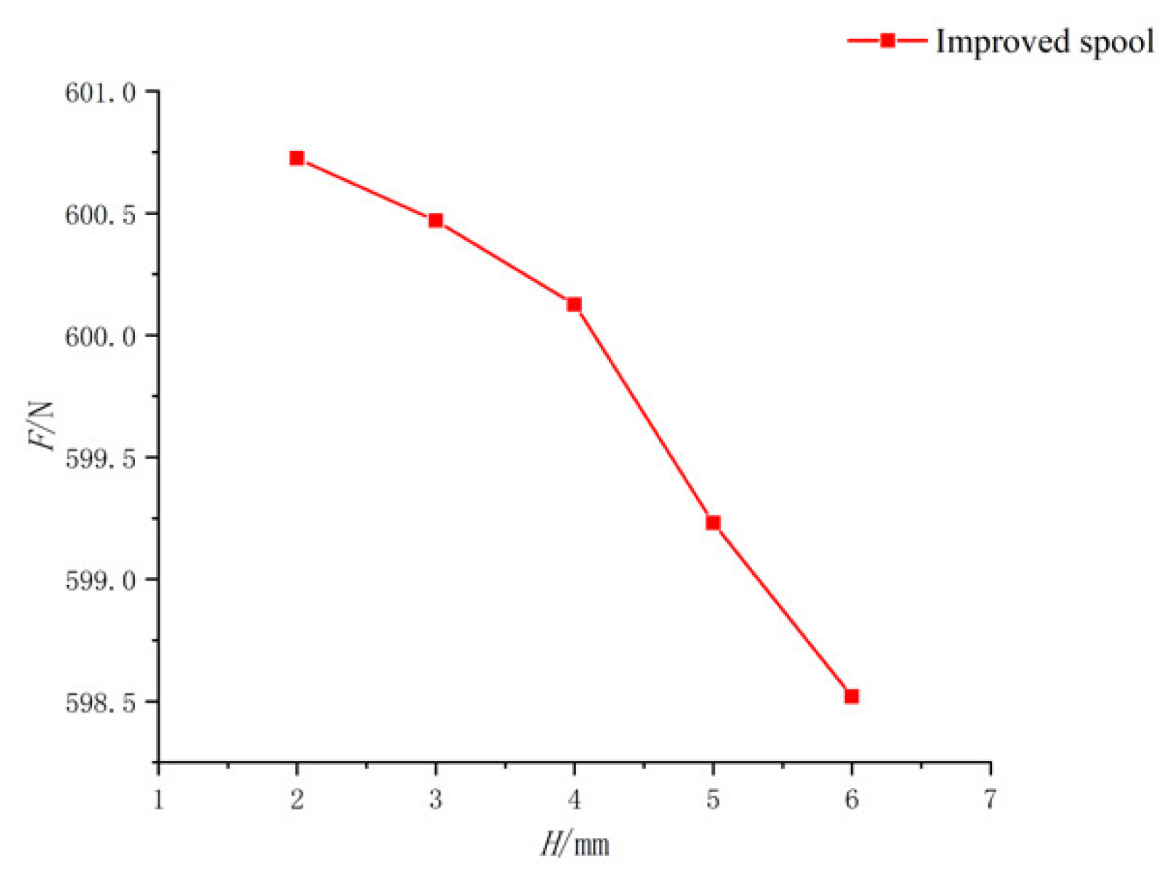
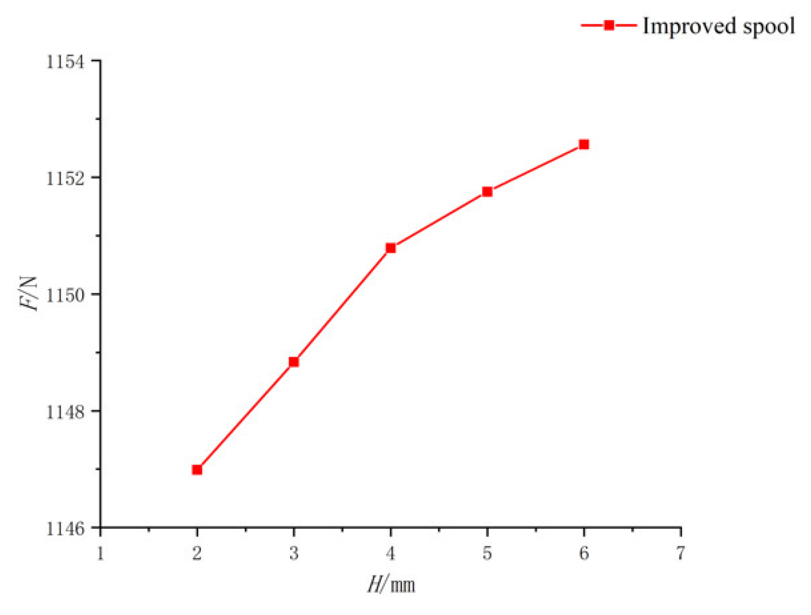
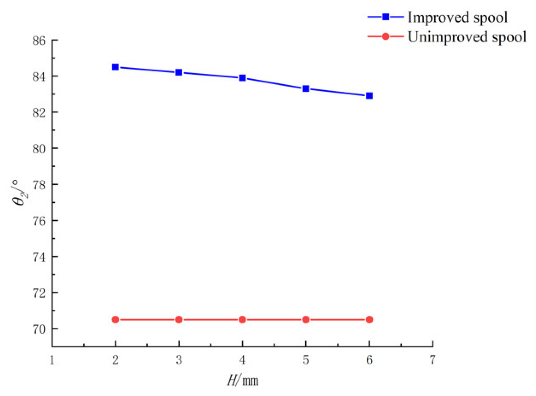
When fixed, D and D₁ remained unchanged; with increasing H, the jet angle increased, the flow force compensation effect increased and the flow force decreased, accordingly. Increasing H had a positive effect on flow-force compensation and was conducive to the stability of the spool.

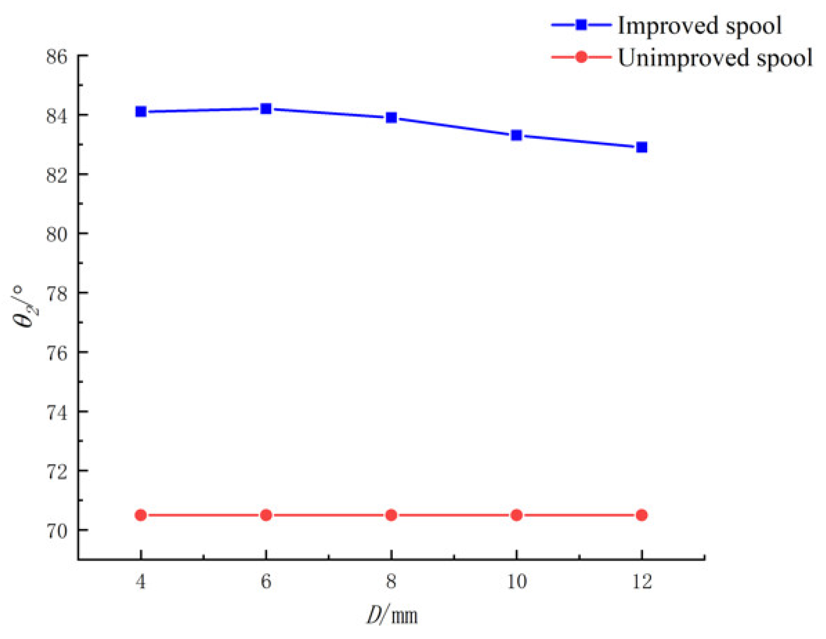
(3)

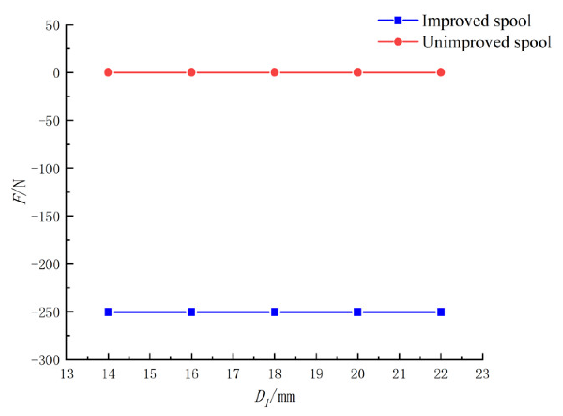
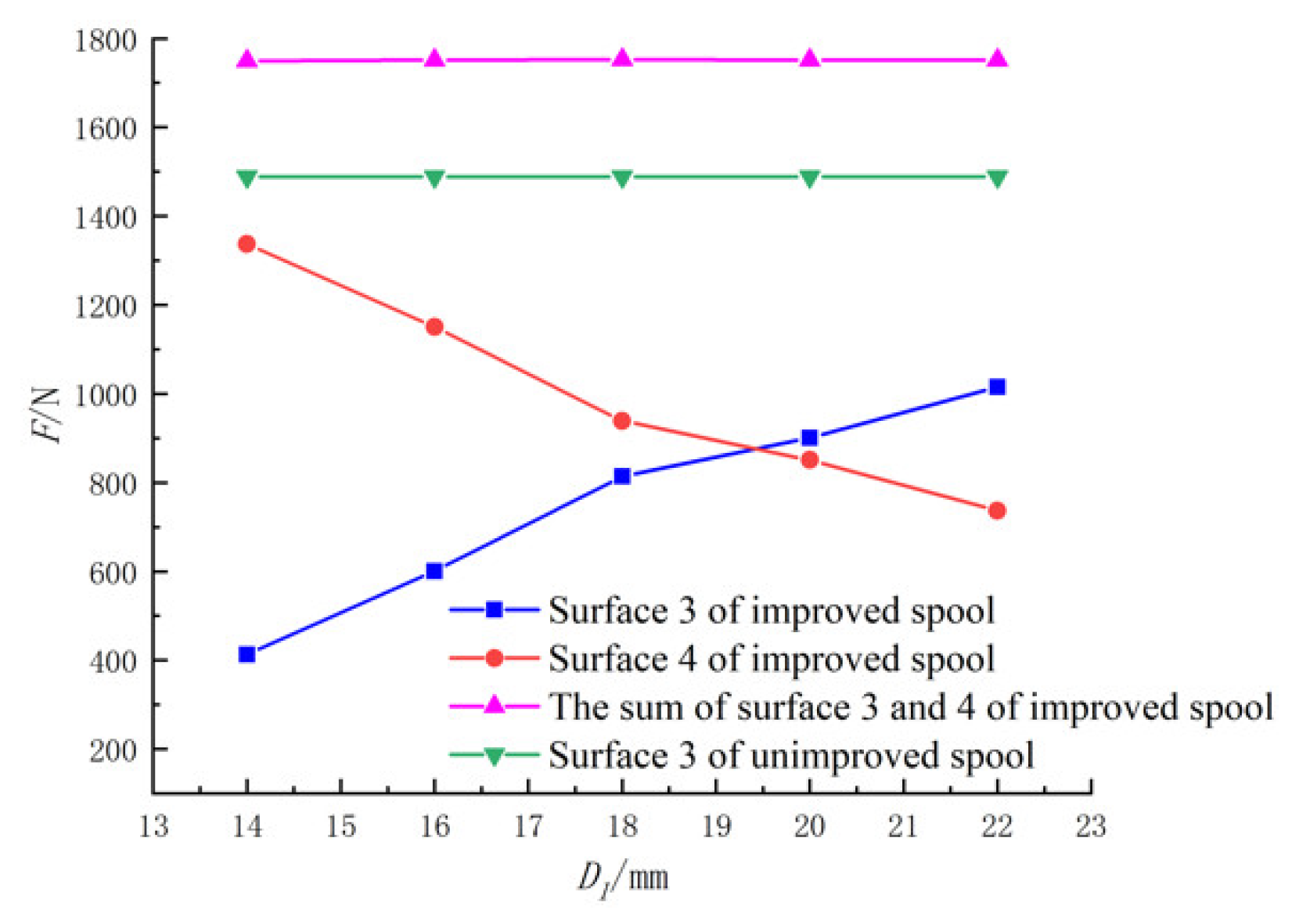
When fixed, D and H remain unchanged; with increasing D₁, the jet angle increased and the flow force decreased. When D₁ was too large, the jet angle increased slowly or even decreased, and the flow force increased.

Further, the flow force of the spool under different opening diameters was analyzed experimentally. The experiment results were consistent with the simulation results, which verifies the effectiveness of the improvement. The compensation coefficient was defined and calculated. The calculation results show that the absolute value of the compensation coefficient of the improved spool was less than that of the unimproved spool. The improved spool had obvious flow-force compensation characteristics. With increasing pressure difference, the absolute value of the compensation coefficients of the two spools became larger, the compensation effect decreased, and the compensation characteristic became unstable. When the pressure difference was small, the compensation effect was more apparent.