1. Introduction
Greenhouse gas (GHG) emissions into the atmosphere must be reduced to mitigate global warming. In the 1990s, hydrofluorocarbons (HFCs) were adopted as zero ODP alternative refrigerants to chlorofluorocarbons (CFCs) and hydrochlorofluorocarbons (HCFCs), but they were listed as greenhouse gases in the Kyoto Protocol [
1]. In 2014, a calendar to phase out HFCs from several sectors and applications was established under the (F-gas) Regulation (EU) No 517/2014 [
2]. Among various refrigeration and air conditioning applications, commercial refrigeration systems commonly used in supermarkets contribute remarkably to GHG emissions. Higher HFC leakages in these systems are expected in these systems due to the higher refrigerant charge and probability of failure [
3].
For many years, R404A and R507A have been refrigerants extended in supermarket refrigeration systems [
4], but both refrigerants have very high global warming potential (GWP) values, 3943 and 3985, respectively. According to the beginning of 2020, a ban on stationary refrigeration systems using refrigerants with GWP values equal to or greater than 2500 (with some exceptions) came into effect from the EU F-gas Regulation. Therefore, manufacturers and users of supermarket refrigeration systems have tried to consider alternative refrigerants with lower GWP to replace R404A. There are different refrigerants available for this purpose, such as carbon dioxide [
5], ammonia and hydrocarbons [
6] and HFC mixtures and HFC/HFO mixtures [
7]. One of the HFC/HFO mixtures developed and commercialized is R449A. With a lower GWP value than R404A and still non-flammable and zero-ODP fluid, this refrigerant can perform as a drop-in/light retrofit replacement in supermarket refrigeration systems [
8].
It is common to analyze the performance of refrigeration systems by using conventional approaches, including analytical and experimental methods. Today, it is common to employ artificial intelligence methods to solve complicated refrigeration and air conditioning systems. An artificial neural network (ANN) can be employed [
9,
10] as this method has excellent approximation capabilities. The use of ANNs makes it possible to predict the desired output even in complex refrigeration and air conditioning systems. Its simplicity, speed, and ability to model a multivariable system are the main advantages of using ANNs [
11,
12].
The ANN method was employed by Hosoz and Ertunc [
13] to predict the energy parameters in a cascade vapour compression refrigeration system using R134a. Their results revealed that the ANN had great potential to model the performance of the system reliably. Tong et al. [
14] developed an ANN model to study the performance of a refrigeration system. Using this technique, they proposed a refrigeration system control method for saving energy when working in part-load conditions. Onder [
15] employed ANN modelling to analyze the energy consumption and the thermodynamic aspects of a refrigeration system. The modelling results were in excellent agreement with the actual data. Li et al. [
16] developed an ANN model to design a control strategy for indoor air temperature and humidity in a direct expansion air conditioning system. They employed 169 sets of experimental data and modelled the performance of the system. Belman-Flores et al. [
17] developed an ANN model to investigate the energy performance of a small refrigeration system using R134a, R450A and R513A. The ANN model predicted the system’s performance well and helped to compare the system’s performance using R450A and R513A with R134a for a replacement.
For this transition to low GWP refrigerants, only a few studies have proposed and validated an ANN model as a tool to evaluate the energy performance and the suitability of the new alternative. Moreover, there is a lack of studies that consider field test data for feeding the ANN model despite its potential for predicting the operation and possible failures. Therefore, this study aims to develop ANN models for two different supermarket refrigeration circuits operating at low temperature (LT) and medium temperature (MT), and investigate the capability of R449A to be used as an alternative refrigerant to R404A in an existing installation. The model outputs are used to evaluate the system’s energy performance for both refrigerants and experimental results. Finally, these results are also used to analyze the carbon footprint reduction caused by refrigerant replacement.
2. Characteristics of R404A and R449A
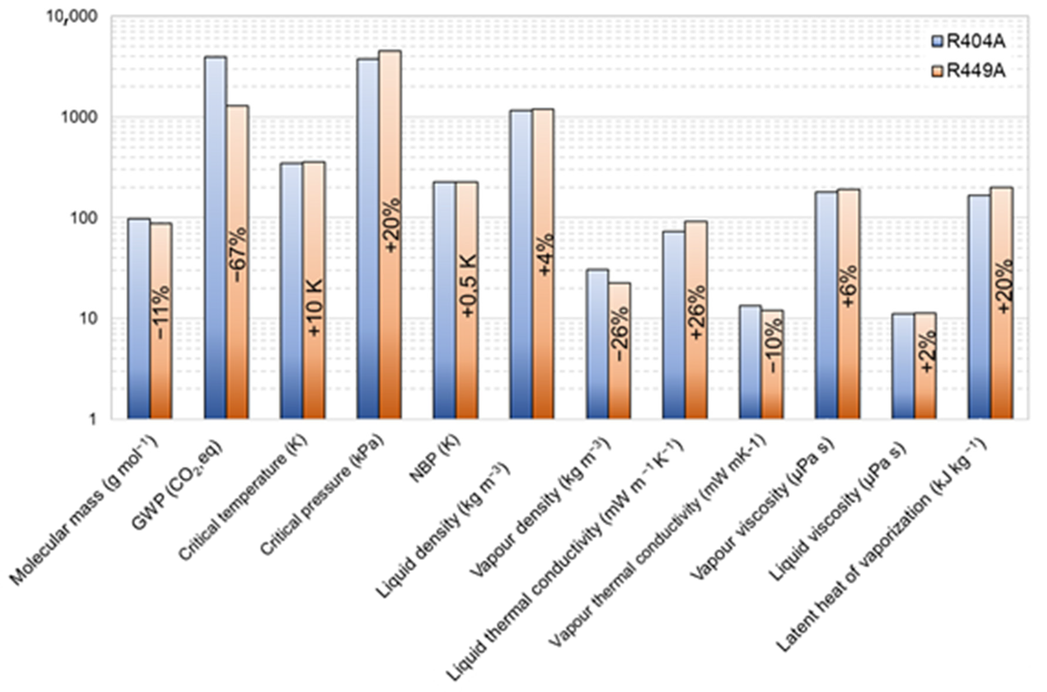
R449A is one of the first blends using hydrofluoroolefins (HFOs) in their composition since it is composed of R32, R125, R1234yf, and R134a at a mass concentration of 24.3/24.7/25.3/25.7, respectively. Both R404A and R449A are non-flammable and non-ozone-depleting refrigerants.
Figure 1 represents the comparison between the most representative properties of both refrigerants [
18]. When necessary, the reference temperature has been set to 0 °C. R449A has a much lower GWP value (about three times), and it can decrease the direct contribution to global warming through leakages. The replacement refrigerant, R449A, has a higher critical temperature and pressure than R404A, indicating the reduction in the power required for the compression process.
Although the vapor density of R449A is lower, it has a higher latent heat of vaporization than R404A and could compensate for the lower mass flow rates of R449A. Therefore, almost a similar cooling capacity for both refrigerants could be anticipated. At 0.1 MPa, the R449A temperature glide of 5.7 °C indicates that it cannot be considered a near-azeotropic mixture. For R404A, instead, this parameter only reaches 0.8 °C. The relatively higher temperature glide of R449A influences the heat transfer performance at the evaporator and condenser.
3. Supermarket Refrigeration System
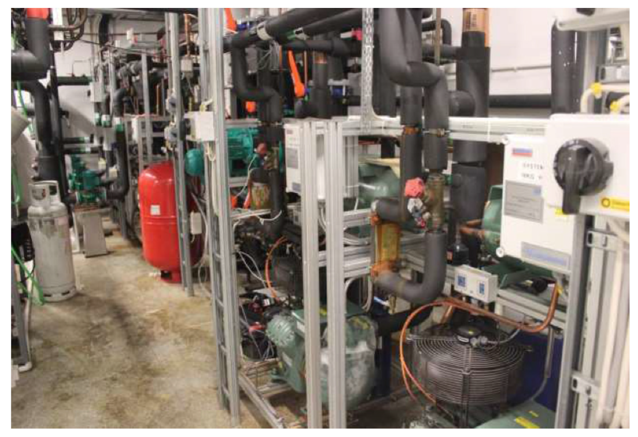
In this study, the measurement data from an indirect supermarket refrigeration system, as shown in
Figure 2 (installed in 2005 in Södertälje, Sweden), were used to compare the performance of the two refrigerants. Each supermarket refrigeration system consists of three parallel circuits to provide the required cooling capacities at low temperature (−35 °C to −25 °C) and medium temperature (−9 °C to −5 °C).
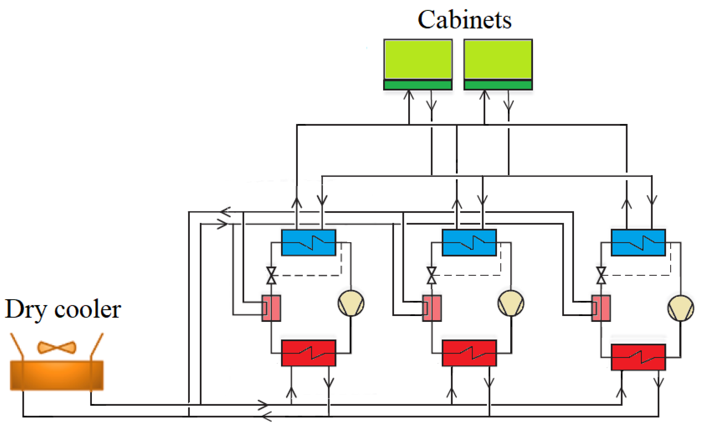
A simplified diagram of the cooling systems is shown in
Figure 3. As can be seen, the refrigeration system delivers cooling to the secondary refrigeration circuits working with CO
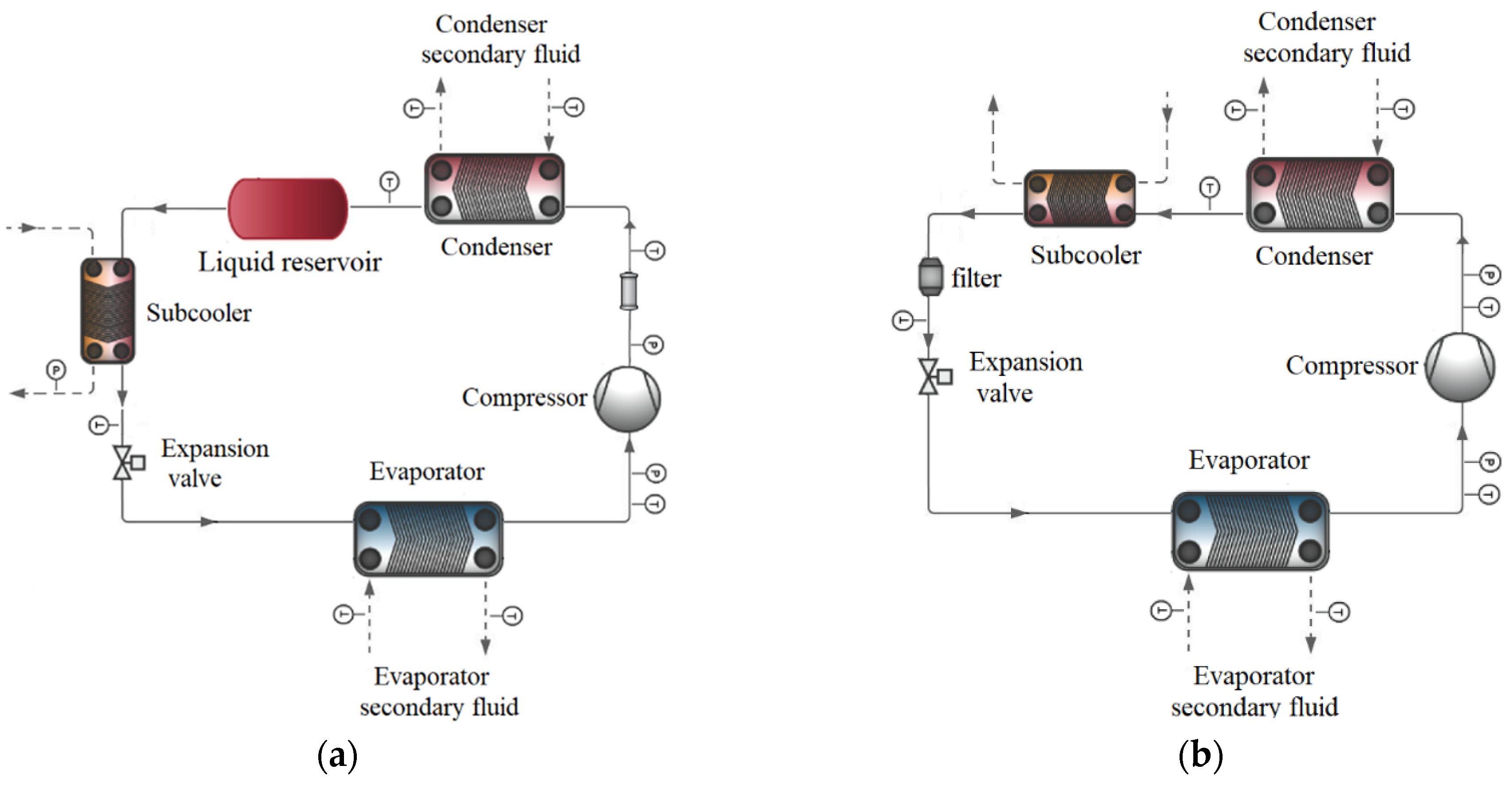
2 and propylene glycol/water mixture (38/62 per volume) in LT and MT circuits, respectively, and the secondary fluid distributes this further to cabinets to cool the products in them. The heat rejected from the connected cabinets is transferred to a dry cooler through a secondary fluid circuit and then is rejected to the ambient. In this study, the analyzed refrigeration system is one of the three refrigeration loops combined in parallel in the cooling system. The schematic of the supermarket refrigeration systems used in LT and MT applications is presented in
Figure 4.
Table 1 represents the details of the components of the refrigeration systems used in this study. Both systems are based on semi-hermetic reciprocating compressors (higher capacity for the MT circuit) and plate heat exchangers. The performance of the two refrigeration circuits using R404A and R449A was monitored and measured for 172 days, and the data at steady-state conditions were selected for this study. The refrigerant charge amount was 12.0 kg for R404A, and it was 12.5 kg when R449A was retrofitted into the supermarket refrigeration system. An electronic expansion valve was adjusted to obtain the correct superheating temperature, and the POE lubricant substitution was performed according to the manufacturer recommendation when retrofitting the refrigerant. The adjustment of the electronic expansion device and the amount of refrigerant charge provided approximately comparable superheating and subcooling degrees.
In the LT circuit, the middle evaporating temperature (calculated as the sum of 1/3 of the dew point temperature and 2/3 of the bubble temperature at the evaporating pressure) varied between −40 °C and −31 °C for both R449A and R404A systems. The middle condensing temperature (vapor quality 0.5) was slightly higher in the R404A system (between 21 °C and 47 °C) than that of the R449A (between 13 °C and 43 °C). The subcooling degree was observed to be 17 + −7 K for the R404A system, while most of the measured subcooling temperature was 29 + −6 K for the R449A. On average, the R449A system operated at higher subcooling temperature than the system using R404A at LT application. Both R404A and R449A systems operated with comparable superheating degrees, varying between 8 K and 11 K.
During the MT system operation, it was observed that the majority of the measured values for the subcooling and superheating temperatures were 3 ± 2 and 7 ± 2 K, respectively. The measured superheating and subcooling temperatures were slightly lower, 1.5 K on average, for when R449A was used as the working refrigerant compared to when the system operated with R404A. A wide range of middle condensing and middle evaporating temperatures was observed when the medium temperature cooling system operated with R404A and R449A. The system operated with slightly higher middle evaporating and middle condensing temperature with R404A compared to R449A. The observed middle evaporating temperature varied between −20 °C and −10 °C for the R449A system compared to the range of −17 °C to −8 °C for the R404A system. On the other hand, the middle condensing temperature changed between 25 °C and 43 °C for the R449A system, while it was in the range from 29 °C to 45 °C for the R404A system.
4. Artificial Neural Networks
The artificial neural network is a non-linear mapping system consisting of large numbers of computational units with connections in a parallel structure and analogous to simplifying biological neurons in a brain [
19,
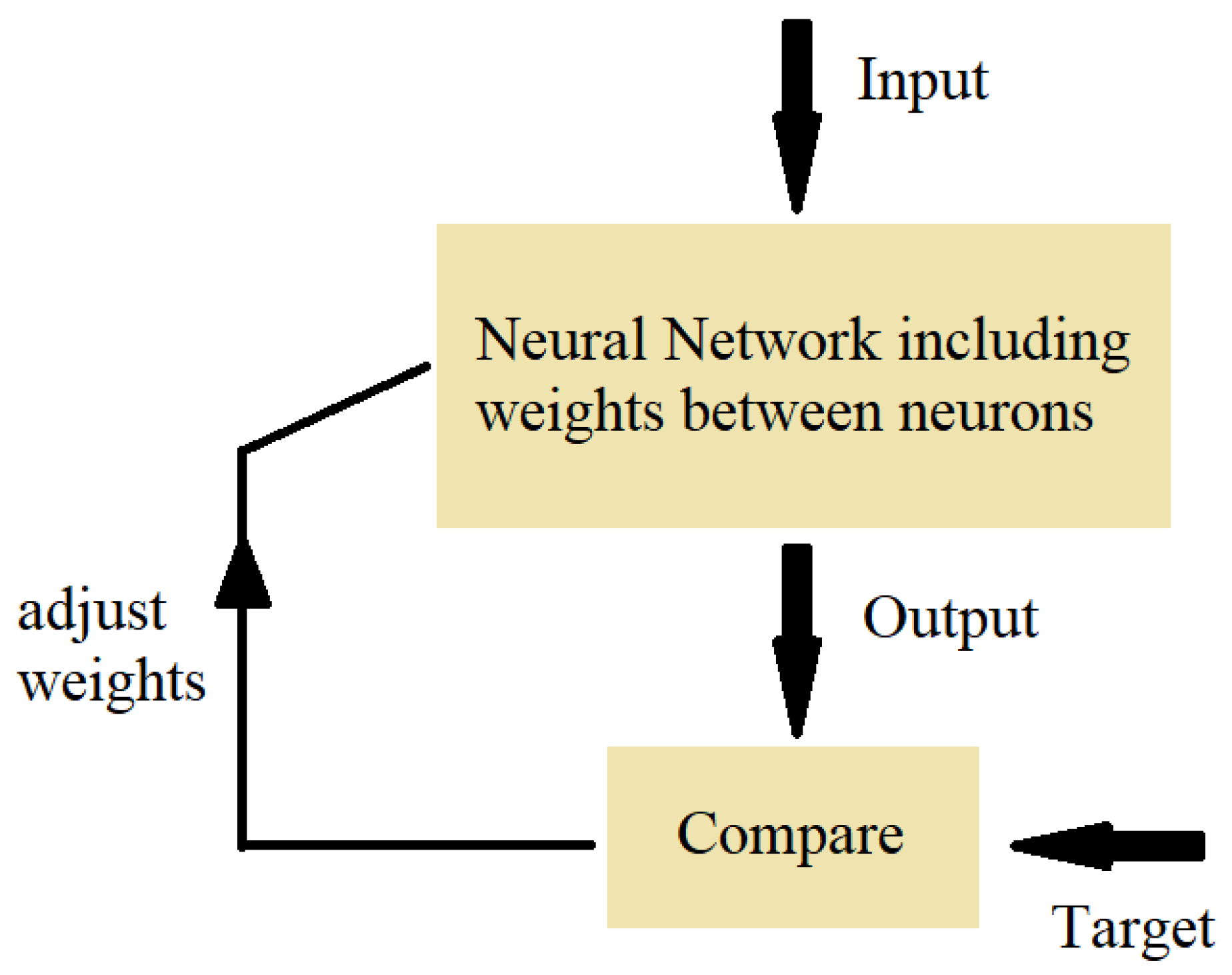
20]. As a flexible and powerful tool for approximation, an ANN commonly consists of three parts: an input layer, a hidden layer(s), and an output layer. The basic principles of ANNs are shown in
Figure 5. An ANN uses the training data to learn the relation between input and output. The system receives inputs; then, each neuron receives weighted results. After summing up all the weighted results and passing through the activation function, the predictive output is delivered [
21]. The sum of the weighted inputs is calculated as presented in Equation (1):
where
P,
wi, and
b are the number of elements, the interconnection weight of the input vector
xi in the preceding layer, and the bias term of the neuron, respectively. The output is then calculated using the sum of the weighted inputs with a bias through an activation function. In this case, the output is obtained as presented in Equation (2).
where
f is an activation function. To train an ANN system, many input-target output pairs are used. The adjustment of the values of connections between the elements is based on comparing the output and the target. This process is repeated until reaching the point that the network output and the target are matched using the optimal set of weights. The error of the modelling is produced by comparing the output of the model with the desired response.
The network used in this study has four inputs, including the middle evaporating and condensing temperatures and the superheating and subcooling temperatures. In the hidden layer, the number of neurons was controlled and adjusted to avoid overfitting. In the output layer, there is only one output. Therefore, three ANNs were designed and trained to predict the values for the output parameters, including the COP, the cooling capacity, and the compressor discharge temperature. The field measurement data were employed to train the model and test the predicted results (75% for training and 25% for testing).
For computational programming of the ANN, Matlab software was employed. The optimal number of hidden layers and neurons for each layer were selected by trial and error. Therefore, no rule was established for this purpose. The neural network performance was controlled using the mean square error (MSE), which is defined as presented in Equation (3).
where
ysim and
yobs are the predicted output and the observed output, and
N is the number of data points. To solve non-linear least squares problems and supervise the learning way called backpropagation, the Levenberg–Marquardt algorithm (LMA) was used [
22,
23]. This algorithm is known as damped least-squares (DLS) method. The LMA, as a commonly used algorithm to solve generic curve-fitting problems, computes derivations according to the training data. To avoid overfitting, the best results according to the validation data found during the previous iterations were remembered by the algorithm. Although the standard backpropagation is known as a slow algorithm, the LMA has been proved to have the fastest convergence on networks.
5. Results and Discussion
The energetic performance of the supermarket refrigeration system using R404A and R449A was measured and calculated. Then, some ANNs were trained using the experimental data. The experimental results were compared with those from the ANN model to validate the ANN model. The experimental and ANN modelling results for the two refrigerants at both LT and MT applications are discussed in this section.
5.1. LT Application
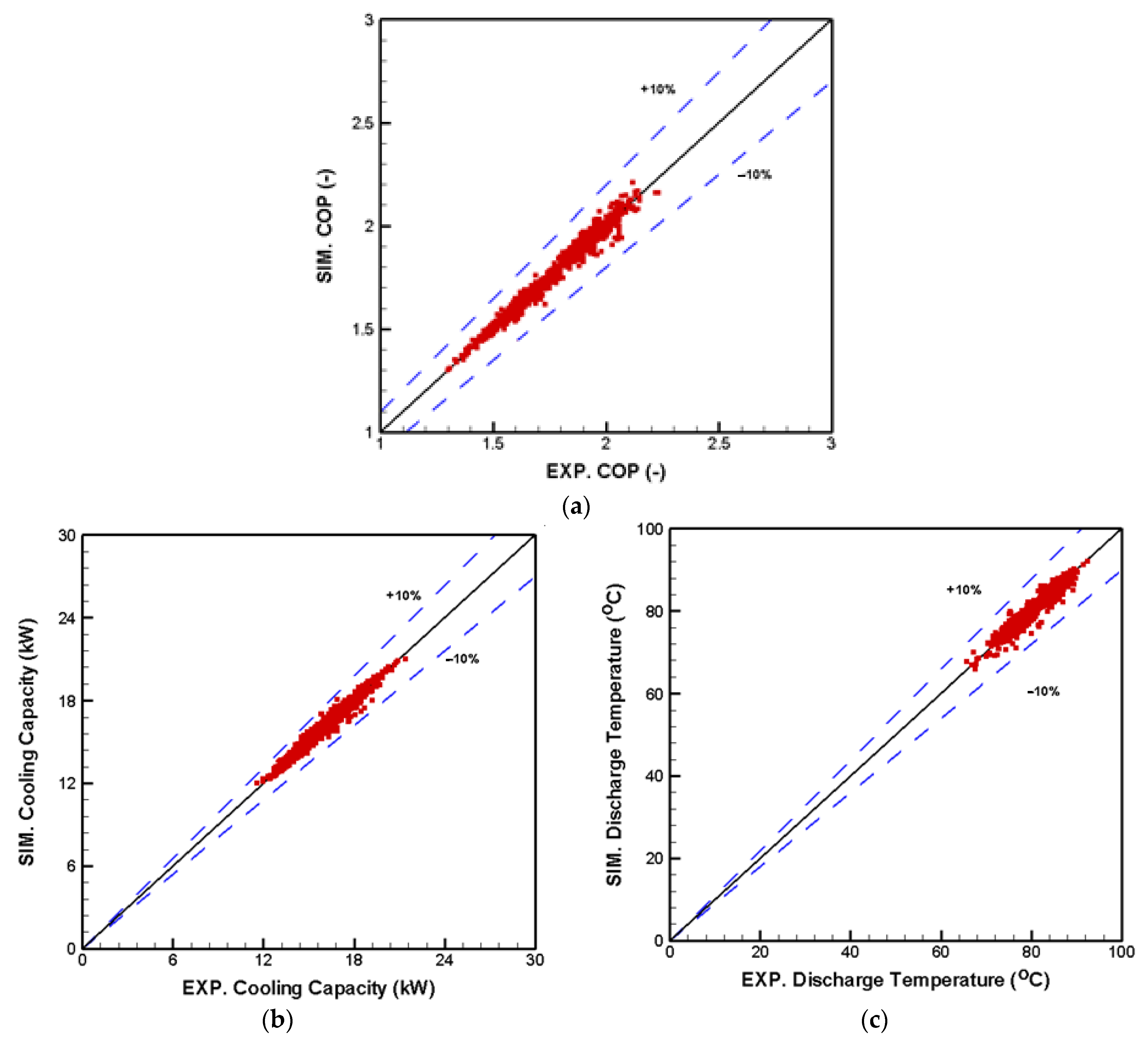
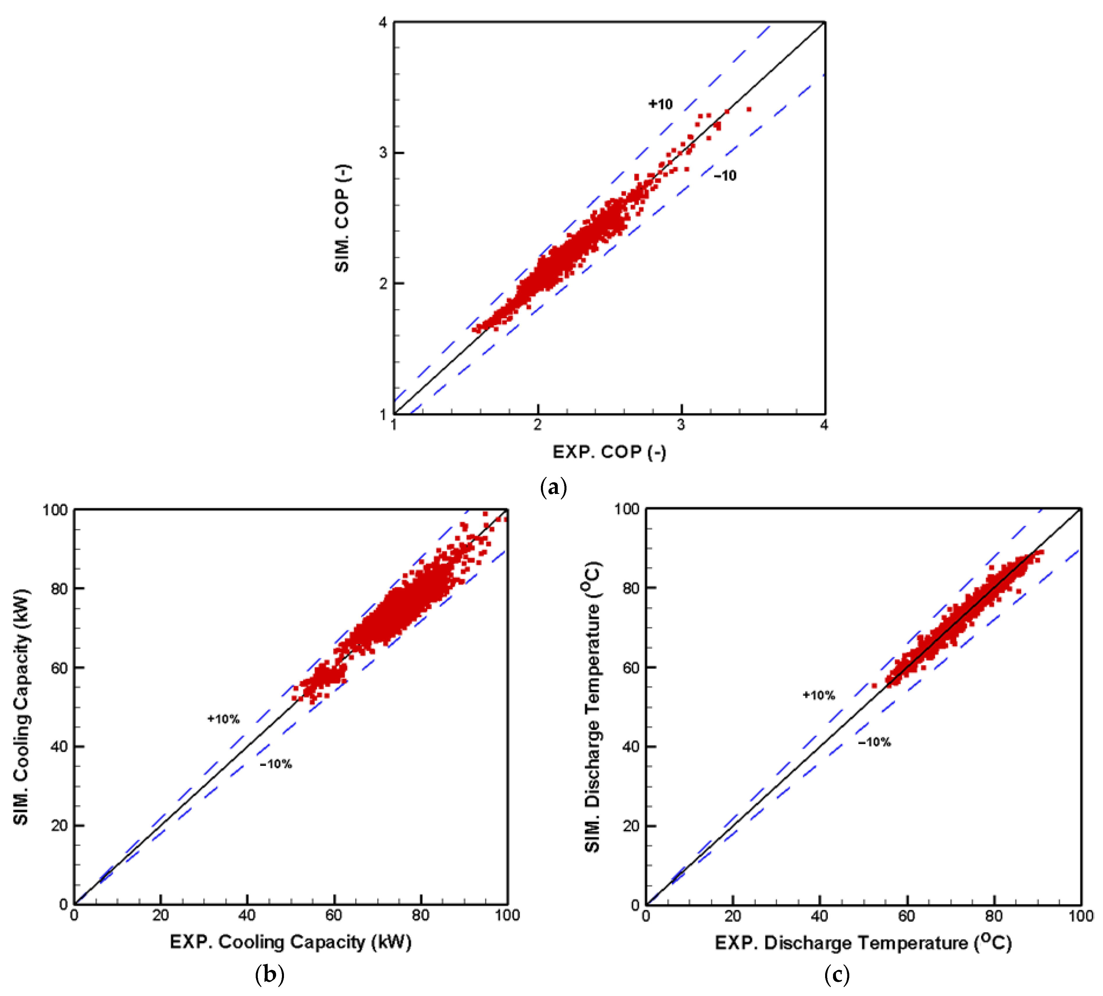
The agreement between the experimental and ANN modelling results for the energetic performance parameters, including the COP, the cooling capacity, and the compressor discharge temperature, is shown in
Figure 6. The vertical axis represents the ANN modelling results, while the horizontal axis shows the experimental values. In each graph, a straight line indicating a perfect prediction and a ±10% error band was used to evaluate the modelling accuracy. Note that for all graphics in
Figure 6, the comparisons were made using the values for both R404A and R449A without distinction. As can be seen, most of the points are within the ±10% error band, indicating an outstanding accuracy of the model. The results demonstrate that the ANN model predicted the energy parameters of the supermarket refrigeration system with high accuracy despite wide ranges of operating conditions.
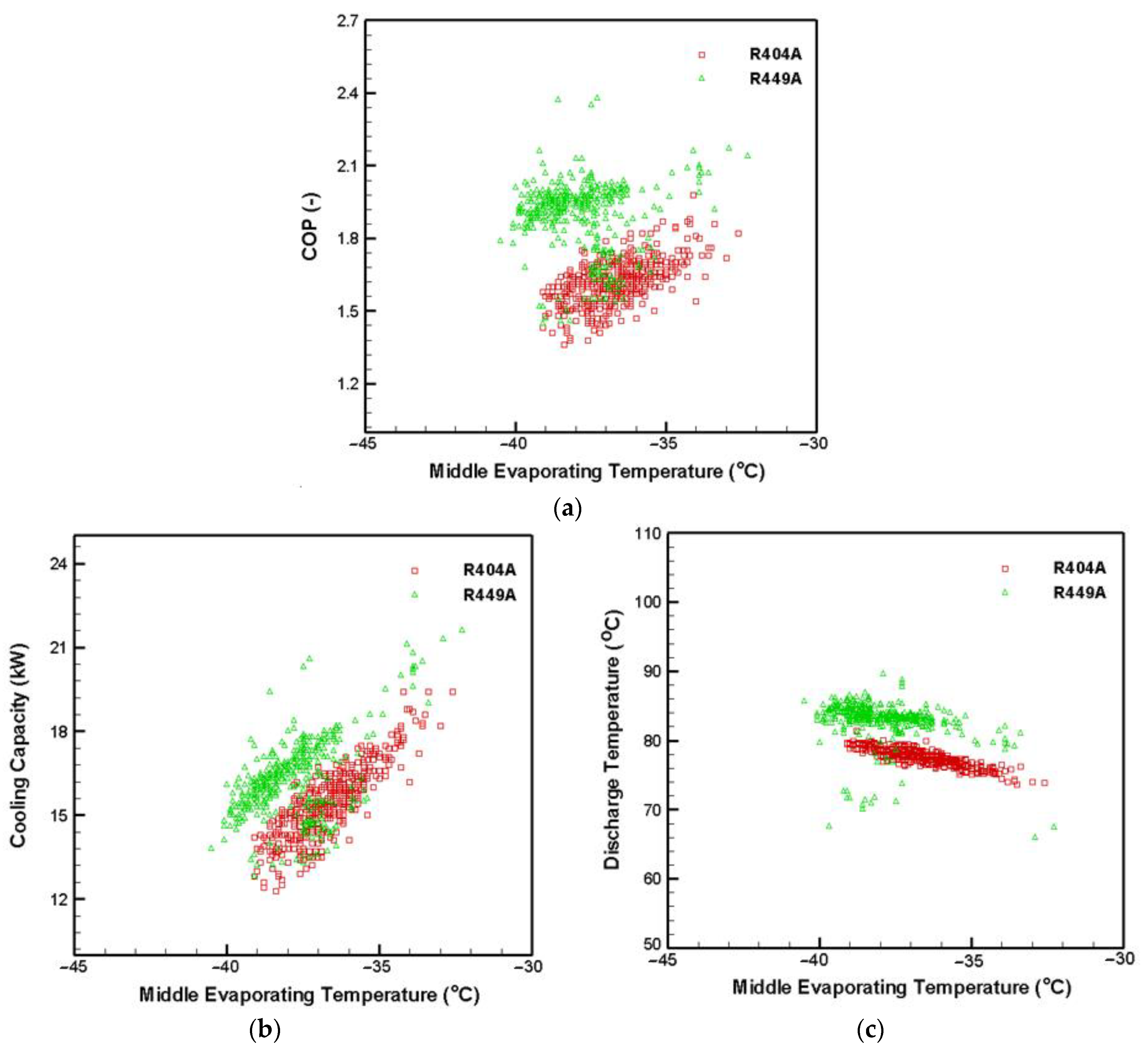
Figure 7 represents the field measurement results of the supermarket refrigeration system for R404A and R449A at the LT application. According to the experimental results, the supermarket refrigeration system exhibited a better performance when operating with R449A than R404A. It is observed that at a constant middle condensing temperature of 30 °C, the cooling capacity increases when using R449A as a substitution to R404A. It is important to note that the supermarket refrigeration system operated with comparable superheating temperatures for R404A and R449A refrigerants at LT case. However, the system experienced different ranges of subcooling temperatures with these two refrigerants. It was observed that the subcooling temperature for R449A is remarkably higher than that of R404A. Over the range of operating conditions, the subcooling temperature for the system using R449A was 12 K higher than that of R404A. The higher cooling capacity of the MT surpasses cabinet thermal requirements, so this excess is used for a higher subcooling in the R449A LT circuit. Then, the positive effect of subcooling temperature can explain the higher COP and cooling capacity values for the system using R449A compared to R404A. It is also observed that the system using R449A has a higher discharge temperature than R404A. For both refrigerants, the maximum average observed discharge temperature (86 °C) is still within the safe limit recommended by the compressor manufacturer and does not affect the compressor lifetime and oil lubricating properties.
As mentioned above, the difference in the subcooling temperature of the two refrigerants can affect the performance of the system. To better judge the influence of R449A as a substitution to R404A, the ANN model is employed to compare R404A and R449A under the same operating conditions.
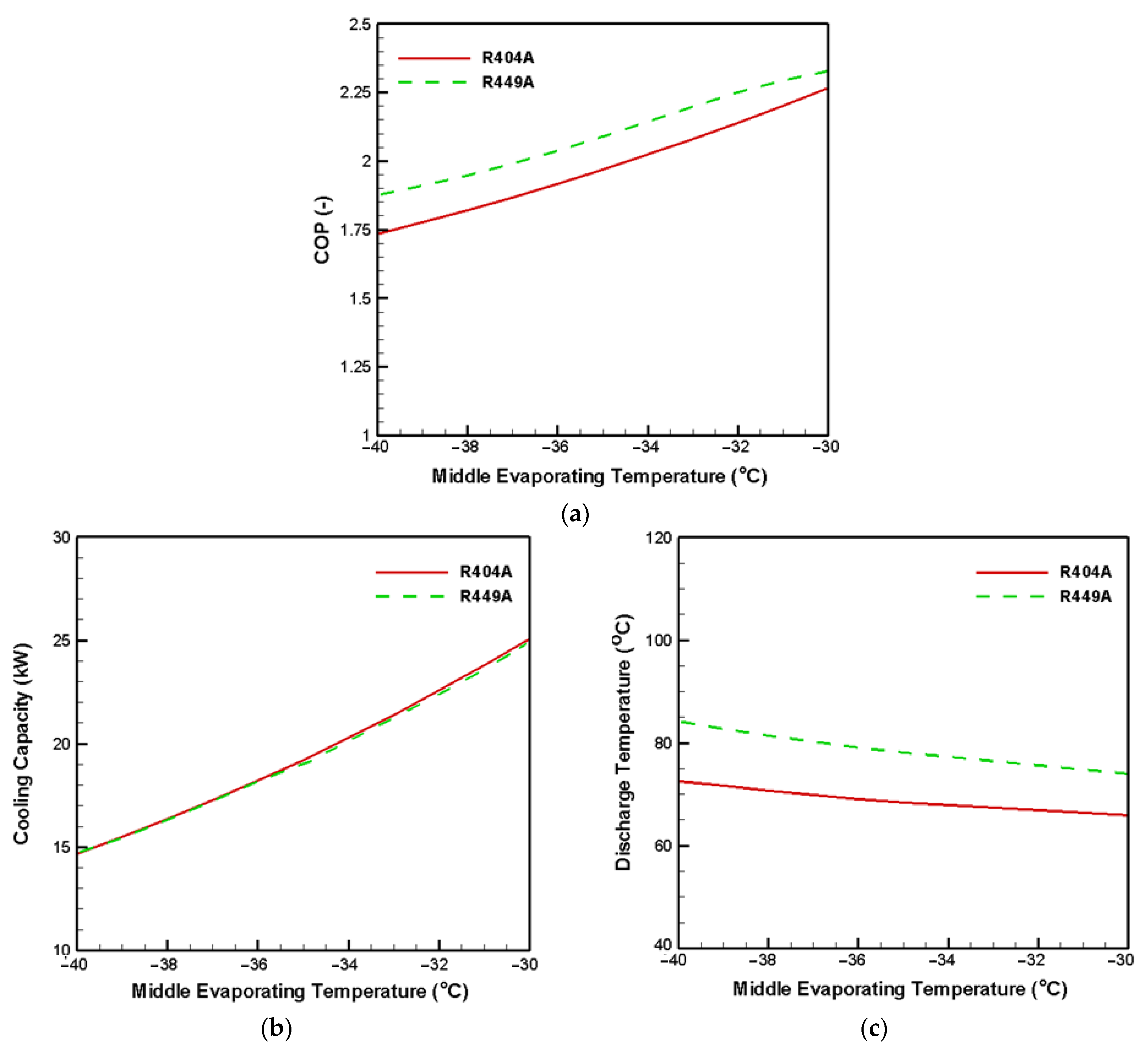
The predicted results of the energy parameters of the supermarket refrigeration system under the same operating conditions at different possible evaporating temperatures is shown in
Figure 8. According to the predicted results, the supermarket refrigeration system using R449A exhibited a better energy performance as it has a higher COP than R404A at different middle evaporating temperatures. However, the cooling capacity was found to be comparable for R404A and R449A. The COP of the system using R449A was predicted to be higher by 10%, on average, than R404A over the middle evaporating temperature range. The modelling results also confirmed that the discharge temperature for R449A is higher than R404A under the same operating conditions, about 10 K on average.
5.2. MT Application
Like the LT case, the ANN model’s accuracy to predict the refrigeration system’s energy performance is evaluated, and the comparison results with the experimental data are presented in
Figure 9. The comparison between the experimental and modelling results revealed that the accuracy of the ANN model is still acceptable, as happened with the LT circuit. Although the deviation of the predicted results from the straight line is observed, most of the points are still within the ±10% error band. Therefore, the ANN model can predict the energy parameters of the supermarket refrigeration system at MT application with acceptable accuracy.
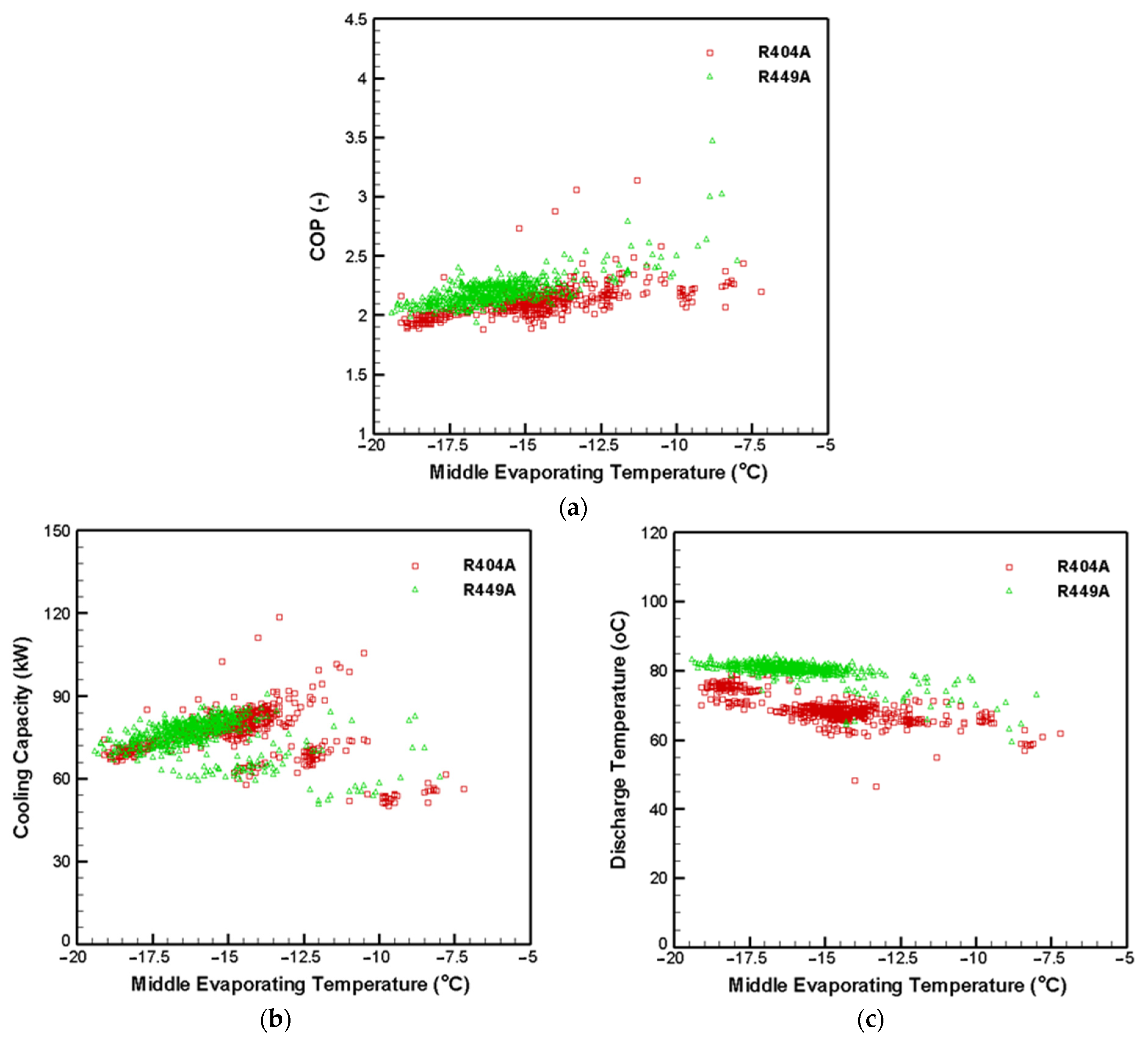
The field measurement results of the supermarket refrigeration system for R404A and R449A at MT application is shown in
Figure 10. The evaluation of the energy parameters as the constant middle condensing temperature of 35 °C revealed that the supermarket refrigeration system has comparable COP and cooling capacity. However, similar to the LT case, R449A increases the compressor discharge temperature compared to R404A. It is also important to note that the higher temperature for the system using R449A may lead to more significant heat losses from the compressor body, which should be considered when calculating its efficiency.
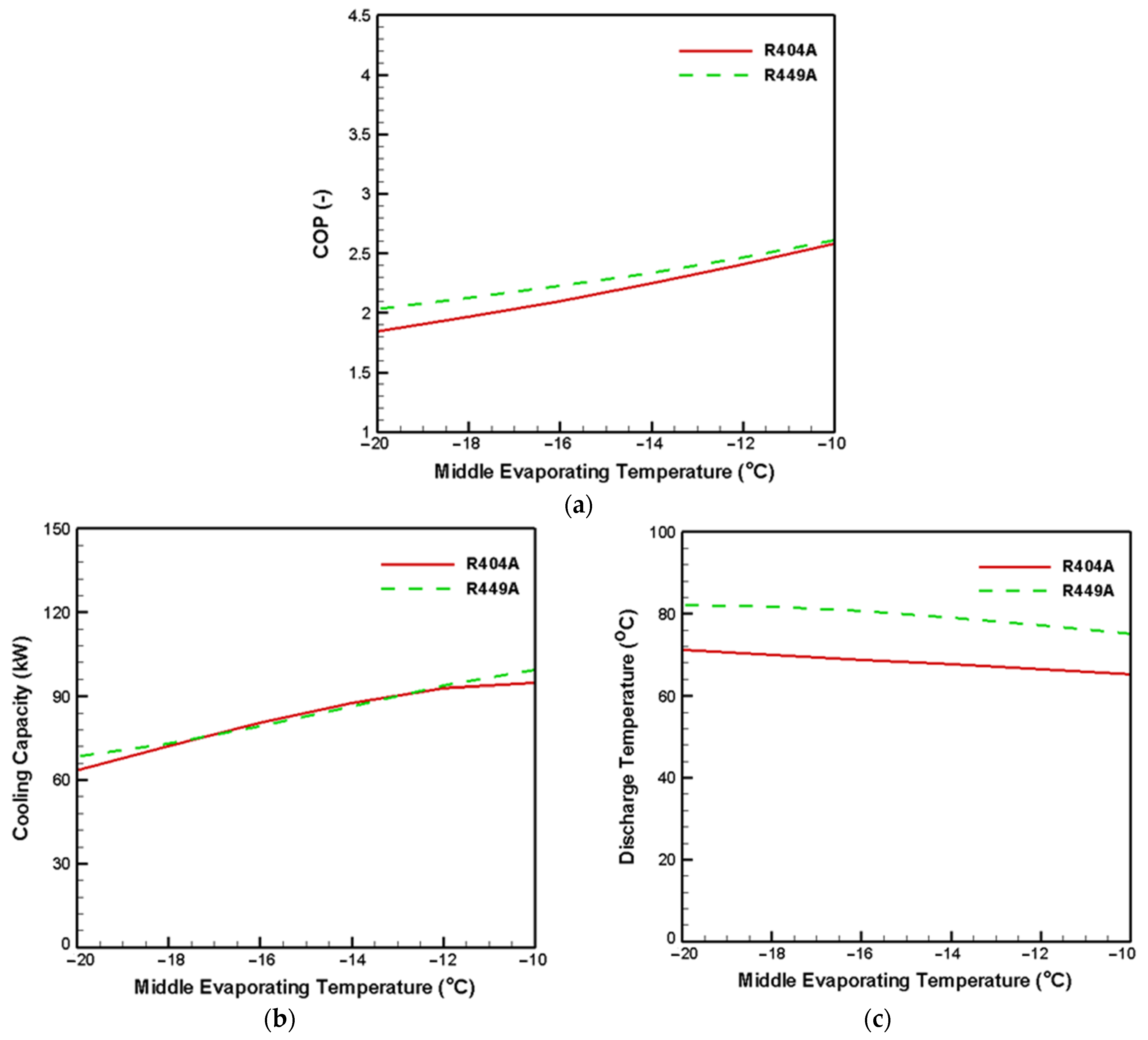
Figure 11 represents the ANN modelling results of the supermarket refrigeration system for R404A and R449A at MT application. The modelling is performed under the same operating conditions to provide a fair comparison between R404A and R449A. It is predicted by the ANN model that the COP of the system using R449A is slightly higher than R404A. At the same time, the cooling capacity is similar for both refrigerants over the middle evaporating temperature range. About 5%, on average, increase in the COP of the system is predicted when the system operated with R449A compared to R404A at MT application. Like the LT application, the compressor discharge temperature for the system operated with R449A is 10 K higher than R404A, while both refrigerants operated within the safe limit recommended by the compressor manufacturer.
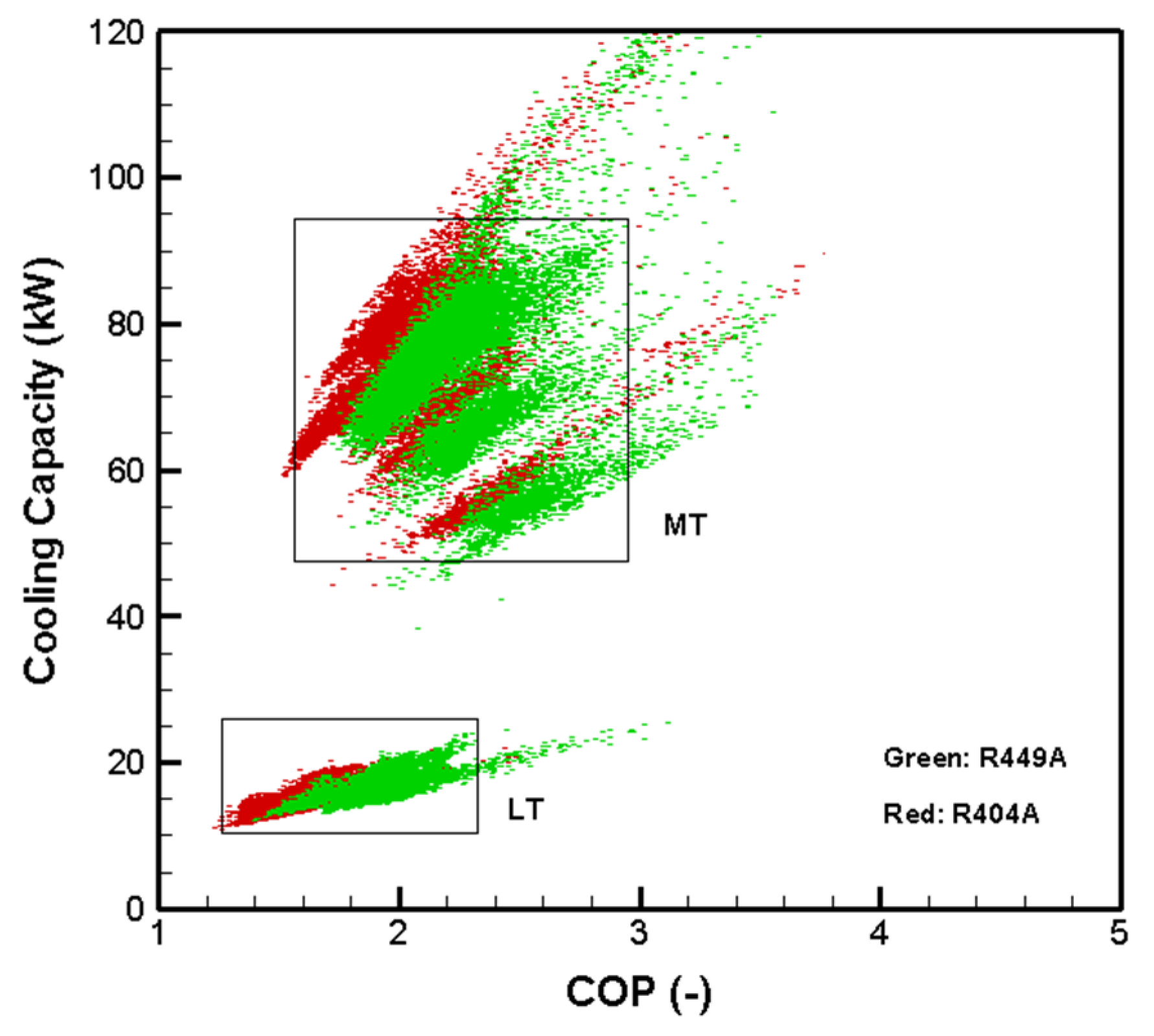
Finally, the cooling capacity versus COP of the supermarket refrigeration system at LT and MT applications is included in
Figure 12 in order to have a complete overview of the comparison. The field measurements showed that the COP of the system for the majority of the measured points varied between 1.2 and 2.4 for the LT application, and it was from 1.5 to 3.0 for the MT case. The system’s cooling capacity was between 10 kW and 25 kW for the LT application, and it changed between 50 kW and 95 kW for the MT application.
To explain the better cooling capacity of the system at MT application, it should be noted that the displacement of the compressor used at MT was 185 m3 h−1. In comparison, it was 84.5 m3 h−1 at LT application. Usually, supermarkets have higher cooling requirements in medium (fresh food and drinks) than in low temperature, food freezing. Hence, the higher refrigerant mass flow rate caused by higher refrigerant density is the main reason for the higher cooling capacity of the supermarket refrigeration system.
Then, COP is higher at MT applications because the pressure ratio is diminished. Therefore, the specific compression work is significantly reduced, and other influencing parameters such as compressor efficiency improved. On average, the pressure ratio of the MT system was 4.5 and 5.6 for R404A and R449A systems, respectively, and that of the LT system was 9.8 and 13.23 for R404A and R449A systems, respectively. Then, the compressor efficiencies were also influenced by the pressure ratio, benefitting the MT circuit.
5.3. Carbon Footprint Analysis
In this study, the total equivalent warming impact (TEWI) analysis is employed to estimate the CO
2 equivalent (CO
2.eq) emissions. The direct and indirect emissions resulting from the refrigerant leakages and electricity consumption, respectively, during the refrigeration unit operation [
24]. To calculate TEWI, the heat pump’s lifespan and the recovery factor are considered 15 years and 0.7, respectively, and the annual leakage rate is assumed to be 12% [
8,
25]. The indirect emission factor depends on the sources of energy used for electricity generation. As this parameter differs from country to country, six countries with various indirect emission factors are selected to evaluate the CO
2.eq emissions. The indirect emission factor value is taken from ref. [
26]. It is noted that the carbon footprint of the MT system is studied in this section, and the power consumption of the supermarket refrigeration system, used in the calculation of the CO
2.eq emissions, belonged to the case when the middle evaporating temperature was −15 °C. This temperature was selected as the average operating middle evaporating temperature in the system. So, as an example condition, the corresponding power consumption was extrapolated to 15 years to estimate the system’s carbon footprint.
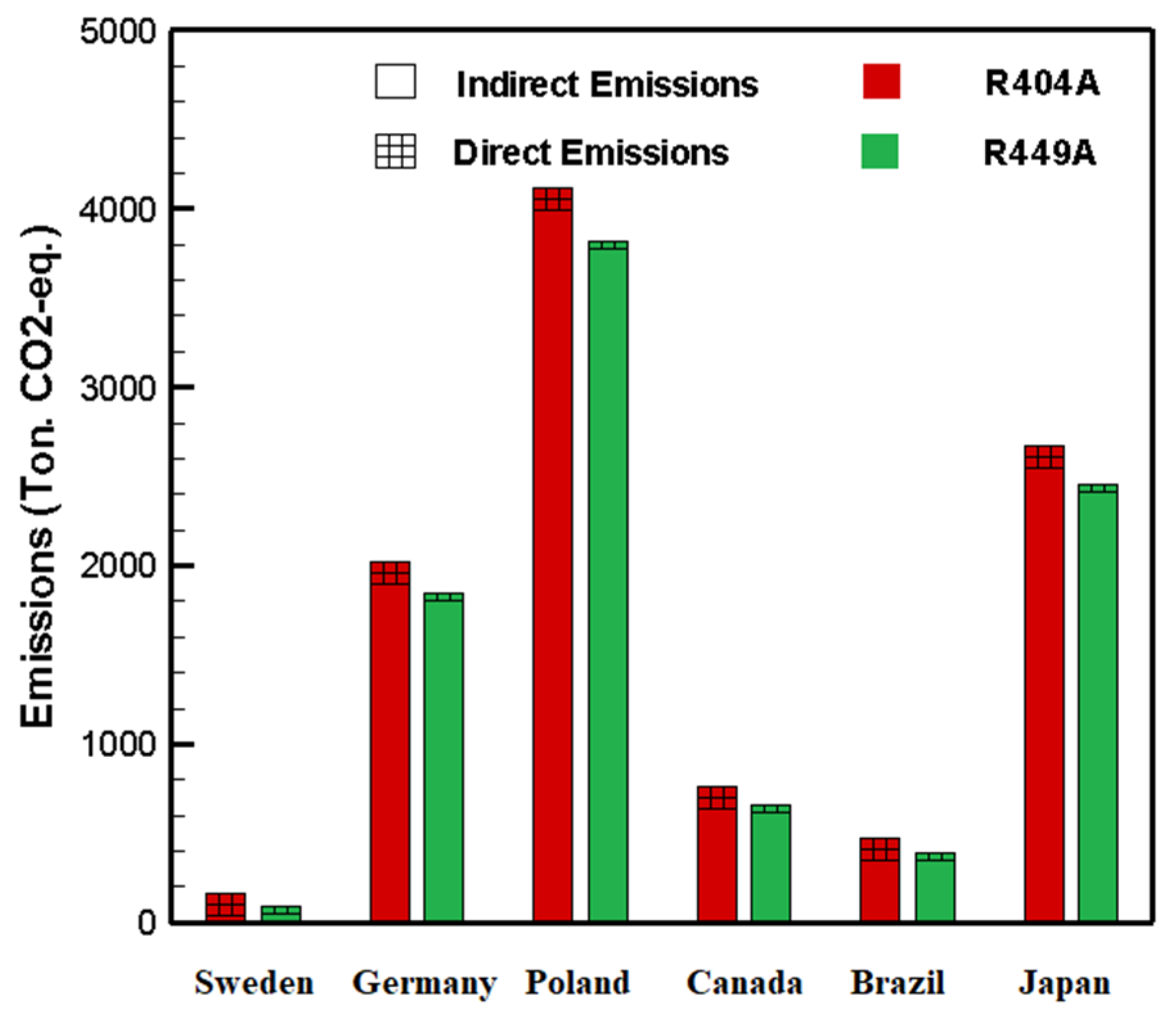
Figure 13 represents the total CO
2.eq emissions of the supermarket refrigeration system operated with R404A and R449A. R404A has a higher direct contribution to CO
2.eq emissions than R449A due to the higher GWP values (about three times) of R404A than R449A. According to the results, R449A has a lower contribution in total CO
2.eq emissions. It means that the phase-out of refrigerants with high GWP values, such as R404A from the commercial refrigeration system, can reduce direct emissions. These results also indicate that the energy sources for electricity generation significantly contribute to the indirect emissions from the supermarket refrigeration system. When the primary sources of electricity are renewable clean energy, the amount of CO
2.eq emissions for each kWh would be much lower than in a country where the primary source of electricity generation is fossil fuels. It can explain much lower total CO
2.eq emissions in a country such as Sweden, with an emission factor value of 0.012 kgCO
2.eq kWh
−1, compared to other selected countries. The presented results support the statement that both the phase-down/out of refrigerants with high GWP values and moving toward clean energy sources for electricity generation are required to mitigate the carbon footprint in the commercial refrigeration industry.
6. Conclusions
A field measurement study and ANN modelling were performed to evaluate the capability of R449A to be used as a lower GWP alternative to R404A in a supermarket refrigeration system. The indirect supermarket refrigeration system comprises two circuits operating at low and medium temperatures. As the operating conditions were different when using R404A and R449A in the refrigeration systems, an ANN model is employed to learn the system’s behavior and make it possible to compare the performance of the two refrigerants. The experimental results were used to train some ANN models to predict the energetic performance of the system under the same operating conditions. The ANN modelling results, supported by the experimental ones, revealed that the use of R449A as an alternative to R404A improves the system’s performance. The COP of the system increases by 10% and 5%, on average at LT and MT, respectively. The cooling capacity was predicted to be almost similar for both refrigerants, and the compressor discharge temperature was predicted to be higher with R449A by almost 10 K. The environmental impact analysis confirmed that R404A has a significant contribution on CO2.eq emissions, and the refrigerant replacement can reduce the emissions from the supermarket refrigeration system.
Author Contributions
Conceptualization, M.G., A.M.-B., P.M.; methodology, M.G., A.M.-B., B.E.B.; formal analysis, M.G.; investigation, M.G., A.M.-B.; resources, M.G., A.M.-B., B.E.B.; data curation, M.G., P.M., J.R.; writing—original draft preparation, M.G.; writing—review and editing, A.M.-B., B.E.B.; visualization, M.G.; supervision, R.K.; funding acquisition, R.K. All authors have read and agreed to the published version of the manuscript.
Funding
Morteza Ghanbarpour acknowledges the financial support of the Swedish Energy Agency and the Swedish Refrigeration Cooperation Foundation, KYS. Additionally, Adrián Mota-Babiloni acknowledges R+D+i project PID2020-117865RB-I00 and grant IJC2019-038997-I, both funded by MCIN/AEI/10.13039/501100011033.
Institutional Review Board Statement
Not applicable.
Informed Consent Statement
Not applicable.
Data Availability Statement
Not applicable.
Acknowledgments
Morteza Ghanbarpour acknowledges the financial support of the Swedish Energy Agency and the Swedish Refrigeration Cooperation Foundation, KYS. Additionally, Adrián Mota-Babiloni acknowledges R+D+i project PID2020-117865RB-I00 and grant IJC2019-038997-I, both funded by MCIN/AEI/10.13039/501100011033.
Conflicts of Interest
The authors declare no conflict of interest.
Nomenclature
| b | bias |
| f | activation function |
| N | number of data points |
| P | number of elements |
| w | interconnection weight |
| x | input vector |
| ysim | predicted output |
| yobs | observed output |
| Abbreviations | |
| ANN | artificial neural network |
| CFC | chlorofluorocarbon |
| COP | coefficient of performance |
| EXP | experimental |
| GHG | greenhouse gas |
| GWP | global warming potential |
| HCFC | hydrochlorofluorocarbon |
| HFC | hydrofluorocarbon |
| HFO | hydrofluoroolefin |
| LT | low temperature |
| MSE | mean square error |
| MT | medium temperature |
| NBP | Normal boiling point |
| ODP | ozone depletion potential |
| POE | polyolester |
| SIM | simulation |
| TEWI | total equivalent warming impact |
References
- United Nations. Kyoto Protocol to the United Nations Framework Convention on Climate Change; United Nations: New York, NY, USA, 1997; Available online: https://treaties.un.org/Pages/ViewDetails.aspx?src=TREATY&mtdsg_no=XXVII-7-a&chapter=27&clang=_en (accessed on 21 November 2021).
- European Parliament and the Council of the European Union. Regulation (EU) No 517/2014 of the European Parliament and the Council of 16 April 2014 on Fluorinated Greenhouse Gases and Repealing Regulation (EC) No 842/2006 Text with EEA relevance. Off. J. Eur. Union 2014, 150, 195–230. Available online: http://data.europa.eu/eli/reg/2014/517/oj (accessed on 21 November 2021).
- Francis, C.; Maidment, G.; Davies, G. An investigation of refrigerant leakage in commercial refrigeration. Int. J. Refrig. 2017, 74, 12–21. [Google Scholar] [CrossRef]
- Mota-Babiloni, A.; Navarro-Esbrí, J.; Barragán-Cervera, A.; Molés, F.; Peris, B. Analysis based on EU Regulation No 517/2014 of new HFC/HFO mixtures as alternatives of high GWP refrigerants in refrigeration and HVAC systems. Int. J. Refrig. 2015, 52, 21–31. [Google Scholar] [CrossRef]
- Sawalha, S.; Piscopiello, S.; Karampour, M.; Manickam, L.; Rogstam, J. Field measurements of supermarket refrigeration systems. Part II: Analysis of HFC refrigeration systems and comparison to CO2 trans-critical. Appl. Therm. Eng. 2017, 111, 170–182. [Google Scholar] [CrossRef]
- Heleno Pontes Antunes, A.; Pedone Bandarra Filho, E. Experimental investigation on the performance and global environmental impact of a refrigeration system retrofitted with alternative refrigerants. Int. J. Refrig. 2016, 70, 119–127. [Google Scholar] [CrossRef]
- Mota-Babiloni, A.; Navarro-Esbrí, J.; Barragán, Á.; Molés, F.; Peris, B. Theoretical comparison of low GWP alternatives for different refrigeration configurations taking R404A as baseline. Int. J. Refrig. 2014, 44, 81–90. [Google Scholar] [CrossRef]
- Makhnatch, P.; Mota-Babiloni, A.; Rogstam, J.; Khodabandeh, R. Retrofit of lower GWP alternative R449A into an existing R404A indirect supermarket refrigeration system. Int. J. Refrig. 2017, 76, 184–192. [Google Scholar] [CrossRef]
- Mohanraj, M.; Jayaraj, S.; Muraleedharan, C. Applications of artificial neural networks for refrigeration, air-conditioning and heat pump systems—A review. Renew. Sustain. Energy Rev. 2012, 16, 1340–1358. [Google Scholar] [CrossRef]
- Sowparnika, G.C.; Thirumarimurugan, M.; Sivakumar, V.M. Performance prediction of refrigeration systems by artificial neural networks. Int. J. Adv. Res. Electr. Electron. Instrum. Eng. 2015, 4, 7673–7681. Available online: https://www.ijareeie.com/upload/2015/september/53_Performance.pdf (accessed on 21 November 2021).
- Kalogirou, S.A. Artificial intelligence for the modeling and control of combustion processes: A review. Prog. Energy Combust. Sci. 2003, 29, 515–566. [Google Scholar] [CrossRef]
- Mellit, A.; Kalogirou, S.A. Artificial intelligence techniques for photovoltaic applications: A review. Prog. Energy Combust. Sci. 2008, 34, 574–632. [Google Scholar] [CrossRef]
- Hosoz, M.; Ertunc, H.M. Modelling of a cascade refrigeration system using artificial neural network. Int. J. Energy Res. 2016, 30, 1200–1215. [Google Scholar] [CrossRef]
- Tong, L.; Yin, S.; Xie, Y.; Wang, L.; Yue, X.; Wang, G. Intelligent simulation on refrigeration system using artificial neural network. In Proceedings of the 2010 Sixth International Conference on Natural Computation, Yantai, China, 10–12 August 2010; pp. 1709–1711. [Google Scholar] [CrossRef]
- Kizilkan, O. Thermodynamic analysis of a variable speed refrigeration system using artificial neural networks. Expert Syst. Appl. 2011, 38, 11686–11692. [Google Scholar] [CrossRef]
- Li, N.; Xia, L.; Shiming, D.; Xu, X.; Chan, M.Y. Steady-state operating performance modelling and prediction for a direct expansion air conditioning system using artificial neural network. Build. Serv. Eng. Res. Technol. 2012, 33, 281–292. [Google Scholar] [CrossRef]
- Belman-Flores, J.M.; Mota-Babiloni, A.; Ledesma, S.; Makhnatch, P. Using ANNs to approach to the energy performance for a small refrigeration system working with R134a and two alternative lower GWP mixtures. Appl. Therm. Eng. 2017, 127, 996–1004. [Google Scholar] [CrossRef]
- Lemmon, E.W.; Huber, M.L.; McLinden, M.O. NIST Standard Reference Database 23: Reference Fluid Thermodynamic and Transport Properties-REFPROP, Version 9.1; National Institute of Standards and Technology, Standard Reference Data Program: Gaitersburg, MD, USA, 2013. [Google Scholar]
- Şencan, A. Performance of ammonia–water refrigeration systems using artificial neural networks. Renew. Energy 2007, 32, 314–328. [Google Scholar] [CrossRef]
- Alamir, M.A. An artificial neural network model for predicting the performance of thermosacoustic refrigerators. Int. J. Heat Mass Transf. 2021, 164, 120551. [Google Scholar] [CrossRef]
- Jiang, H.; Liang, K.; Li, Z.; Zhu, Z.; Zhi, X.; Qiu, L. A sensor-less stroke detection technique for linear refrigeration compressors using artificial neural network. Int. J. Refrig. 2020, 114, 62–70. [Google Scholar] [CrossRef]
- Di Benedetto, R.M.; Botelho, E.C.; Janotti, A.; Ancelotti Junior, A.C.; Gomes, G.F. Development of an artificial neural network for predicting energy absorption capability of thermoplastic commingled composites. Compos. Struct. 2021, 257, 113131. [Google Scholar] [CrossRef]
- Kannaiyan, M.; Govindan, K.; Gowthami Thankachi Raghuvaran, J. Prediction of specific wear rate for LM25/ZrO2 composites using Levenberg–Marquardt backpropagation algorithm. J. Mater. Res. Technol. 2020, 9, 530–538. [Google Scholar] [CrossRef]
- European Committee for Standardization/Technical Committee. SS EN 378-1: 2016 Refrigeration Systems and Heat Pumps—Safety and Environmental Requirements—Part 1: Basic Requirements, Definitions, Classification and Selection Criteria; Bsi. Group: London, UK, 2016. [Google Scholar]
- Life Cycle Climate Performance Working Group. Guideline for Life Cycle Climate Performance v.1.2; International Institute of Refrigeration: Paris, France, 2016; Available online: https://www.buildup.eu/en/practices/publications/guideline-life-cycle-climate-performance (accessed on 21 November 2021).
- Grid Electricity Emissions Factors v.1.4—September 2020. 2020. Available online: https://www.carbonfootprint.com/ (accessed on 21 November 2021).
| Publisher’s Note: MDPI stays neutral with regard to jurisdictional claims in published maps and institutional affiliations. |
© 2021 by the authors. Licensee MDPI, Basel, Switzerland. This article is an open access article distributed under the terms and conditions of the Creative Commons Attribution (CC BY) license (https://creativecommons.org/licenses/by/4.0/).


 ,
, 
