Robust L_p-Norm Inversion for High-Resolution Fluid Contents from Nuclear Magnetic Resonance Measurements

Abstract

Fluid content computed from nuclear magnetic resonance (NMR) has proved to be an accurate and reliable tool for petrophysical property estimation. To overcome the limitations of conventional NMR measurements, high spatial resolution NMR (HSR-NMR) has been introduced to achieve the desired resolution for cores of any size. However, inversion of fluid contents from HSR-NMR data suffers from nonreliable measurements at the ends of the detection coil due to the heterogeneities of the magnetic fields caused by the relatively small size of the coil. A robust L_p-norm inversion algorithm, developed for geophysical inverse problems, has been implemented and applied on the inversion of NMR measurements. The estimated fluid content from L_p inversion matches well with the kerogen content in the cores both visually and quantitively. The resolution of the inverted fluid contents is as high as 1 inch. Further testing on the raw data with large derivations demonstrated that reliable results can only be achieved by using L_p inversion with low p’s values within the range of (1, 1.1).

1. Introduction

Source rock cores in oil and gas reservoirs are routinely extracted for a better understanding of the conditions of the reservoirs. Subsurface properties, such as porosity, permeability, lithology, and other fluid-related properties, are measured from cores in the lab. Accurate measurements of these parameters are critical for the plausible estimation of reservoir productivity. However, accuracy is just one aspect of the whole story. Often, the measured data contain various types of errors from different sources such as equipment, spatial or angular coverages, and noises in the measuring environments. Some of these errors are random, and some are due to systematic reasons. In these situations, reliable and robust estimation of the fluid-related properties is the foremost important objective.

Many different methods have been proposed to measure the fluid contents from the core. A thorough discussion of different measurements is beyond the focus of this paper. In this paper, we will focus on the inversion of fluid contents from a non-destructive method, high spatial resolution NMR (HSR-NMR) measurements. Low field NMR has been widely used in the oil and gas industry to study porosity, permeability, fluid saturation, and behaviors in the rock pores [1,2,3,4,5]. For readers who are interested in different approaches to measuring the fluid saturation from cores, they are referred to the paper [6].

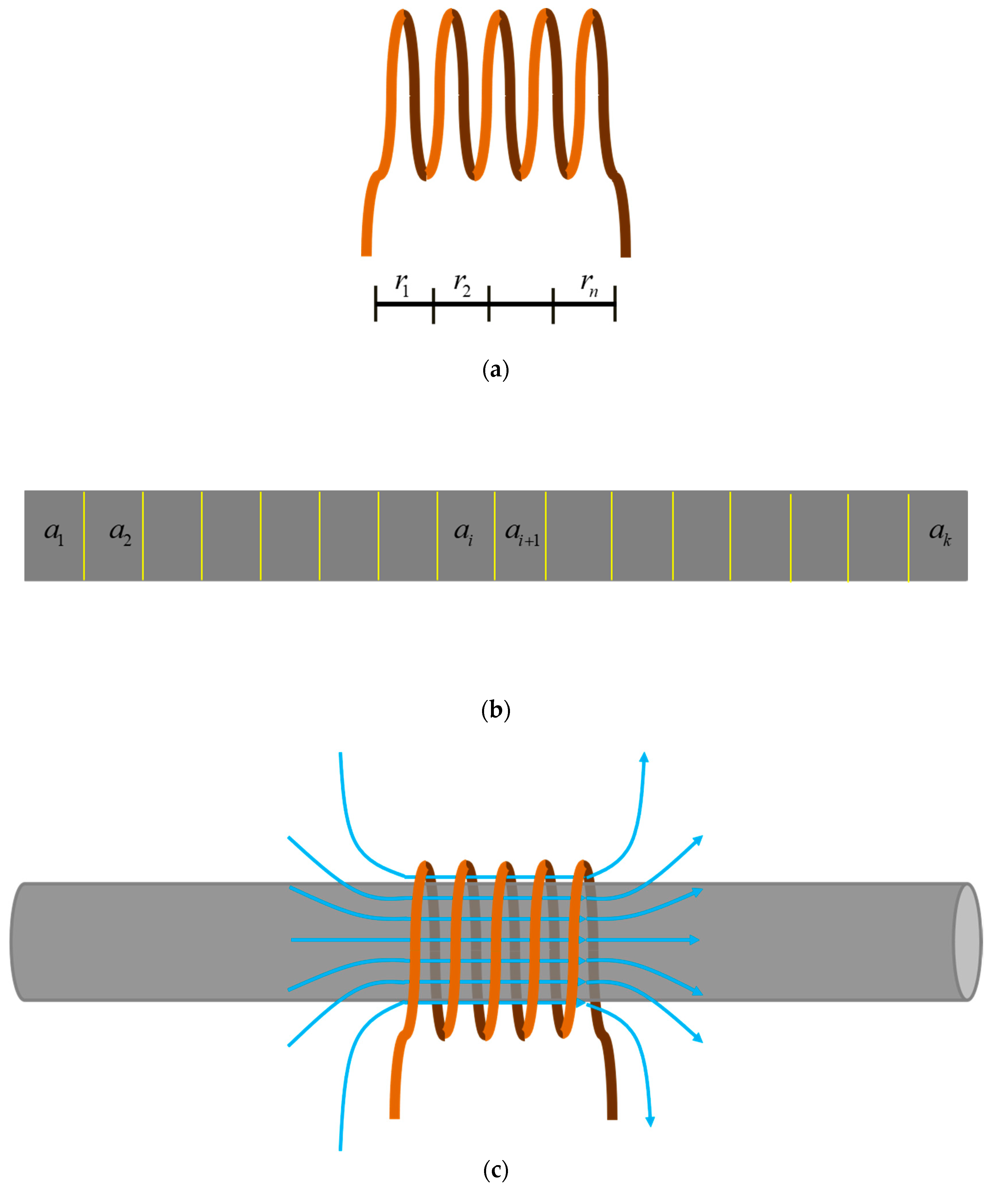
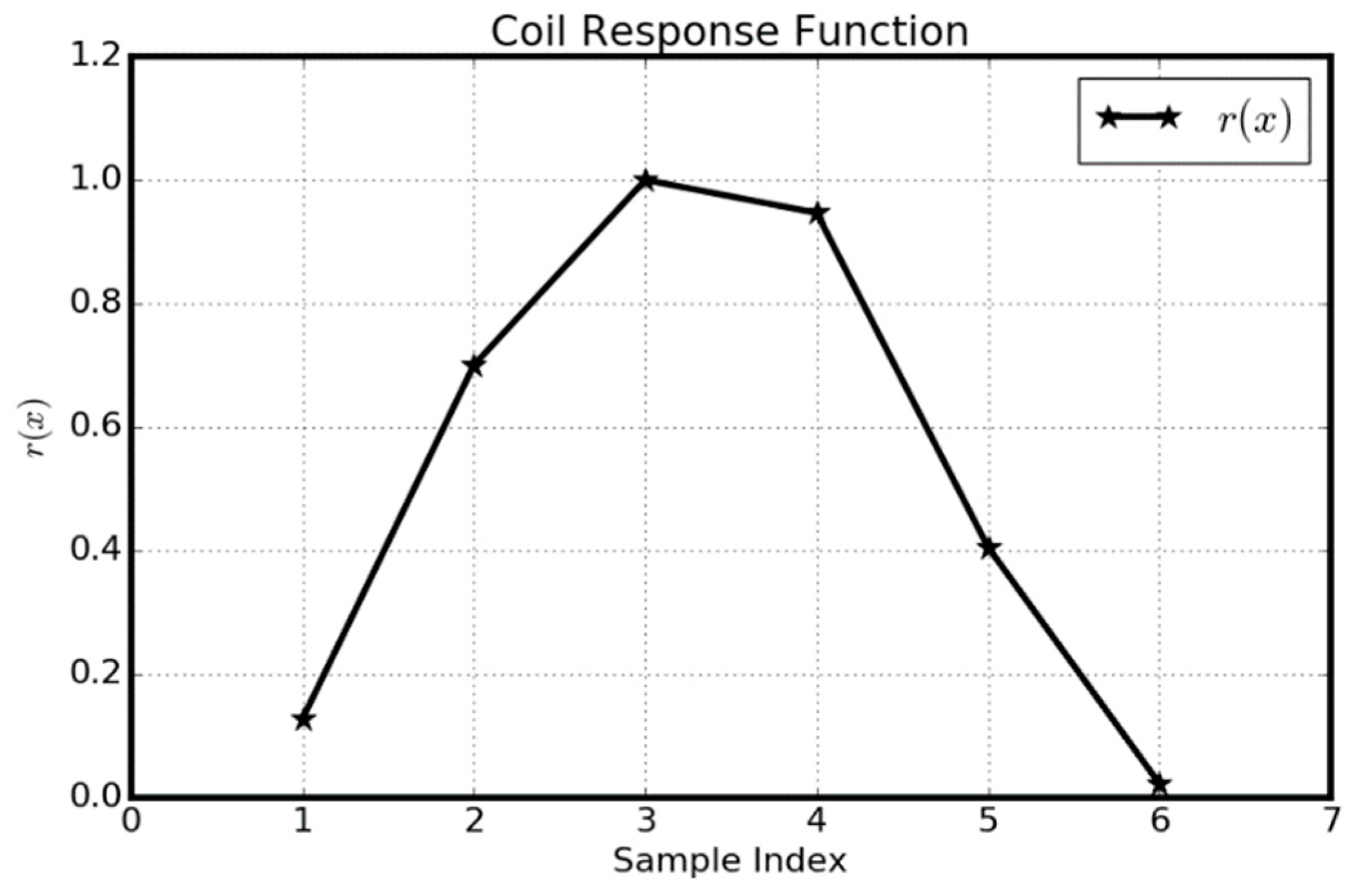
The major elements and main procedures of HSR-NMR measurements are illustrated in Figure 1. Figure 1a shows the coil and the digitized response function r, and Figure 1b shows a long rock sample and the digitized fluid content function a. Figure 1c illustrates the relative position between the coil and the rock sample. The discrete r_i and a_i are defined inside the cells. Note that due to the limited size of the coil, most part of the sample is outside of the coil. The magnetic field produced by the coil shows a significant difference at the middle and on the two ends of the coil.

The main features of HSR-NMR compared with the conventional approach can be summarized as follows: (1) HSR-NMR is a non-destructive technology, which means the same cores are still available for other measurements after NMR. (2) HSR-NMR allows for the same spatial resolution between digitized coils and digitized fluid contents. (3) HSR-NMR measurement can achieve the desired spatial resolution.

There are many similarities between inverting fluid content from NMR data and solving inverse problems in exploration geophysics, for example, in ray-based travel time inversion for macro velocity [7,8], velocity inversion using finite-frequency travel time [9,10,11], post-migration imaging velocity tomography [12], and waveform inversion [13,14]. Extensive research has been performed, and highly effective algorithms have been developed to solve complicated model-building problems in practice [8,13,15,16]. These inversion problems share similar features with the inversion of fluid content from NMR data in terms of noise identification, mitigation of noise impacts, and inversion robustness and accuracy.

Table 1. Comparison of different inversion schemes.

Method	Optimization Function	Pros/Cons	Applications
L2 norm	$C\left(m\right)=\frac{1}{2}{\Vert Am-\tilde{d}\Vert }^2$	Straight forward formulation and implementation. Most widely used. Usually the first choice of inversion. Can not handle non-Gaussian noise and sensitive to large data noises.	Travel time and waveform inversion in geophysics with careful pre-processing of data. Medical imaging and tomography.
Lp norm	$\begin{array}{l}C\left(m\right)=\frac{1}{p}{\Vert Am-\tilde{d}\Vert }^p,\\ 1\le p\le 2\end{array}$	Implementation more complicated. Iterations are needed. Can handle non-Gaussian noise and mitigate impacts of large data noises. Usually gives robust and reliable results.	Travel time and waveform inversion in geophysics with large data errors. Tomography of velocity and density with uncertainties.
Mixed norms	$\begin{array}{l}C\left(m\right)=\frac{1}{p_1}{\Vert Am-\tilde{d}\Vert }^{p_1}\\ +\frac{1}{p_2}{\Vert m-m_0\Vert }^{p_2}\end{array}$	Special implementations are needed. Iterations are needed. Can handle non-Gaussian noise and mitigate impacts of large data noises. Usually gives robust and reliable results. Can include more a prior information.	Waveform inversion in geophysics with a prior information for constraints. Can include model information from other sources.

below compares some advantages and disadvantages of several most often used inversion schemes with mainly focusing on geophysical tomography and similar problems. For a comprehensive review, the readers are referred to [14].

The major contributions of this paper are outlined as follows. First, we use both numerical geophysical experiments and NMR field data to confirm that L_p-norm inversion can suppress the impacts of the data with large deviations. Second, quantitative values are suggested for parameter p for typical practical problems with non-Gaussian noise distribution. Third, we demonstrate that L_p-norm inversion can provide accurate and robust results for fluid contents using MMR data measured from the whole core, which are substantially larger than the size of the coil. This last point makes the proposed approach and workflow especially valuable for practice. The proposed HSR-NMR method is generic and does not depend on the lithology or other properties of the core samples. The method is not limited by the short transverse relaxation time and thus is especially useful for tight rocks such as shales, tight sandstones, and tight carbonates.

This paper is organized as follows. We first review the system equation of the NMR measurements and discuss the challenges and issues posed on fluid content inversion. We then review the similarities between geophysical inverse problems and NMR inversion. These similarities enable us to adopt robust inversion schemes developed in the aforementioned areas. One is $L_p$ norm optimization with model space conditioning. We also carry out an in-depth analysis of the advantages of $L_p$ norm inversion. Finally, we demonstrated high accuracy and robustness by applying the inversion approach on field NMR measurements.

Throughout this paper, we will focus on the numerical aspects of fluid inversion. The physical aspects and their interpretations of the variables in the system equation, the input data, and the inverted results can be found in the papers provided in the references.

2. HSR-NMR System Equation and Issues of NMR Inversion

In this section, we will provide a mathematical description of the relationship between the fluid contents in a core and the NMR measurements. Starting with this equation and the deviation between this theoretical relation and the actual setting up of NMR measurements, we will discuss the issues behind NMR inversion. These discussions provide physical justifications for the use of $L_p$ norm inversion that will be discussed and implemented in the next sections.

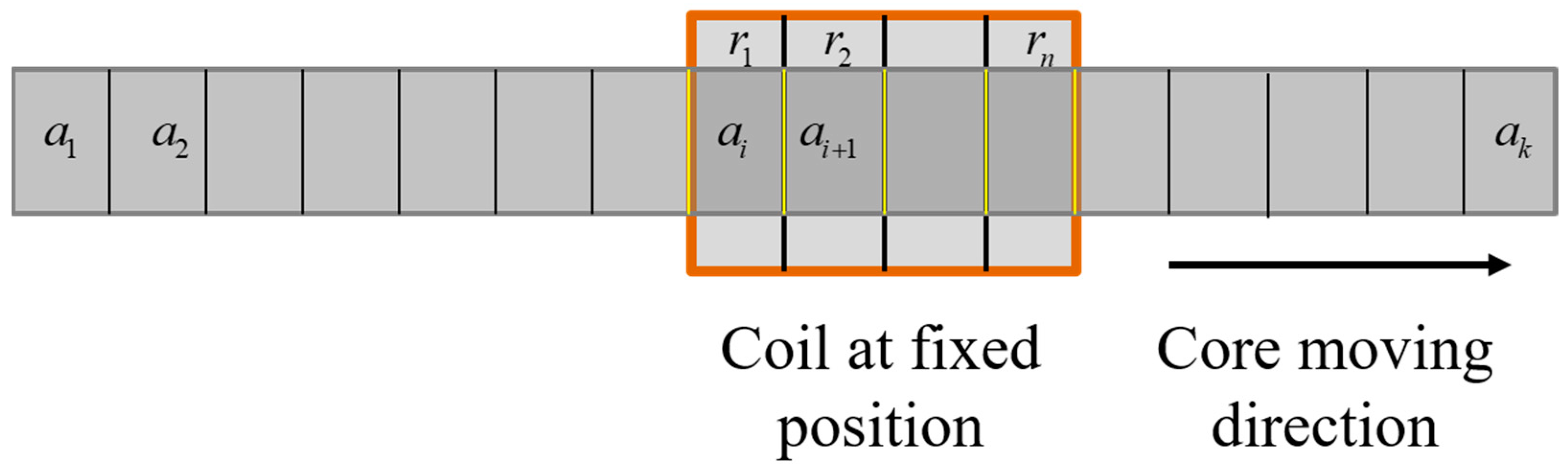
The acquisition of NMR data is illustrated in Figure 1a–c. The whole core is characterized by fluid content function $a\left(x\right)$, and the coil is characterized by the response map function $r\left(x\right)$. $x$ is the coordinate along the axis of the core and the coil, respectively. During NMR measuring (Figure 2), the core is moving to the right while the coil is at the fixed position. At each location of the core, an NMR signal is measured. Assume the fluid content in the core is digitized into k samples, and the response function is digitized into n samples. The relationship between the i^th sample of NMR signal $s_i$ and the fluid contents $a_j$ can be connected by the following discrete linear equations

$$s_1=a_1{r}_1$$

(1)

$$s_2=a_1{r}_2+a_2{r}_1$$

(2)

$$s_n={\displaystyle \sum _{i=1}^n{a}_{m-n+i}{r}_{n-i+1}}$$

(3)

$$s_{k+n-1}=a_k{r}_n$$

(4)

Equation (1) is when the core is at the leftmost position, and Equation (4) is when the core is at the rightmost position. Equation (3) is for general cases. In terms of $m<n$ or $m>k$, we assume $a_i=0$ for $i\le 0$ and $i>n$. To facilitate the implementation of the numerical inversion scheme, the NMR equation can be written in matrix-vector form

$$Ra=s$$

(5)

where $R$ is a function of response map and in the form of a variant Toeplitz matrix [17]. The dimension of $R$ is $\left(k+n-1\right)\times k$. $a$ and $s$ are vectors composed of $a_i,i=1,\cdots ,k$ and $s_i,i=1,\cdots ,k+n-1$, respectively. For example, in the case where k = 9 and n = 5, matrix $R$ and Equation (5) can be written as

$$Ra=\left(\begin{array}{ccccccccc}{r}_1& 0& 0& 0& 0& 0& 0& 0& 0\\ r_2& r_1& 0& 0& 0& 0& 0& 0& 0\\ r_3& r_2& r_1& 0& 0& 0& 0& 0& 0\\ r_4& r_3& r_2& r_1& 0& 0& 0& 0& 0\\ r_5& r_4& r_3& r_2& r_1& 0& 0& 0& 0\\ 0& r_5& r_4& r_3& r_2& r_1& 0& 0& 0\\ 0& 0& r_5& r_4& r_3& r_2& r_1& 0& 0\\ 0& 0& 0& r_5& r_4& r_3& r_2& r_1& 0\\ 0& 0& 0& 0& r_5& r_4& r_3& r_2& r_1\\ 0& 0& 0& 0& 0& r_5& r_4& r_3& r_2\\ 0& 0& 0& 0& 0& 0& r_5& r_4& r_3\\ 0& 0& 0& 0& 0& 0& 0& r_5& r_4\\ 0& 0& 0& 0& 0& 0& 0& 0& r_5\end{array}\right)\left(\begin{array}{c}{a}_1\\ a_2\\ a_3\\ a_4\\ a_5\\ a_6\\ a_7\\ a_8\\ a_9\end{array}\right)=\left(\begin{array}{c}{s}_1\\ s_2\\ s_3\\ s_4\\ s_5\\ s_6\\ s_7\\ s_8\\ s_9\\ s_{10}\\ s_{11}\\ s_{12}\\ s_{13}\end{array}\right)=s.$$

(6)

It should also be pointed out that Equation (5) can also be written as $Ar=s$, where $A$ is composed by the sequence $a_j$ and $r$ is the response map. This duality can be used for calibration of the system response function using known fluid content.

In order to design an optimal numerical scheme for the solution of the NMR equation, we need to have an in-depth understanding of the features of Equation (5). First, the reliability of the information contained in the NMR measurements varies with the changing positions of the core. When the core is at or close to the ends of the coil, due to the inhomogeneous distribution of the magnetic field, the measurements cannot fully reflect the real fluid contents, and therefore, the NMR signals are noisy, and their impacts on the fluid content inversion shall be suppressed.

Secondly, the NMR measurements may contain noise and errors, both of which cannot be completely avoided in field core measurements. If the noises follow Gaussian distribution with an average of zero, ordinary least square inversion is adequate. When the NMR signal contains data samples that deviate from most of the other measurements, then inverted results will be greatly impacted by these large deviations if we fail to identify them. For data processing of a large number of cores in oil and gas exploration, it is challenging and, most of the time, impossible to have full quality control of all the measurements. It is therefore highly desirable for the inversion algorithm to have automatic detection of the high-quality data and to mitigate the impacts of low-quality data or corrupted measurements.

In the next section, we will review some of the inversion algorithms developed for typical geophysical problems such as velocity, impedance, and absorption inversion. The inversion of these geophysical parameters shares similar features to the fluid inversion from NMR data.

3. Robust Inversion for Solving Geophysical Problems

Similar to the NMR Equations (5) and (6), in geophysics, many inverse problems, such as travel time inversion [7,8], global full-waveform inversion [14], and amplitude inversion for absorption coefficients [18] have been investigated. These inverse problems can be formulated as the following linear relations

$$d_i={\displaystyle \sum _{j=1}^N{A}_{ij}{m}_j},i=1,\cdots ,M$$

(7)

where $m_j$ are the discretized model variables or model perturbations, $d_i$ are the discretized observations. $A_{ij}$ is the sensitivity kernel of the $i^{th}$ data measurement $d_i$ with respect to the $j^{th}$ model $m_j$. If the measurements $d_i$ are free of noises and errors, and the linear theoretical relation (7) correctly reflects the true relationship between the model and the data, Equation (7) can be solved using any standard least square-based methods [8,14,19].

In practice, the measured data may contain various types of errors from different sources such as equipment, spatial or angular coverages, and noise in the measuring environments. Some of these errors are random and can be described by Gaussian distribution, and others cannot be described as any systematic distributions. In the case where noise is present, if we assume the same linear relationship between the model and the data, the relationship between data and model can be written symbolically as

$${\tilde{d}}_i={\displaystyle \sum _{j=1}^N{A}_{ij}{m}_j}+{\tilde{n}}_i={\displaystyle \sum _{j=1}^N{A}_{ij}{\tilde{m}}_j},i=1,\cdots ,M$$

(8)

where ${\tilde{d}}_i$ are the actual measurements, and the unknown ${\tilde{n}}_i$ are the errors of the measurements. ${\tilde{m}}_j$ are model parameters that can be inverted using the aforementioned standard methods when the noise is considered part of the input. However, this should be avoided since the information contained in ${\tilde{n}}_i$ about the model may not be useful, and quite often, indiscriminate use of ${\tilde{n}}_i$ as input of inversion may lead to incorrect estimation of the model. Therefore, a robust inversion, which can remove or mitigate the impact of ${\tilde{n}}_i$ and still recover the true $m_j$ rather ${\tilde{m}}_j$, is expected.

To mitigate the impact of the noise on the inversion, we need a cost function that is more tolerant of larger errors [20,21]. This type of inversion is called robust estimation [22]. One such option is to cast the inversion of $m_j$ from (8) into the following L_p-norm optimization problem

$$C\left(m\right)=\frac{1}{p}{\displaystyle \sum _{i=1}^M{\left|{\displaystyle \sum _{j=1}^N{A}_{ij}{m}_j}-{\tilde{d}}_i\right|}^p}$$

(9)

The optimal solution is to find the minimum point of (9). This is given by

$$\frac{\partial C\left(m\right)}{\partial m_k}=0,k=1,\cdots ,N$$

(10)

Using (10), we have

$$\frac{\partial C\left(m\right)}{\partial m_k}={\displaystyle \sum _{i=1}^M\left\{{\left|{\displaystyle \sum _{j=1}^N{A}_{ij}{m}_j}-{\tilde{d}}_i\right|}^{p-1}\mathrm{sgn}\left({\displaystyle \sum _{j=1}^N{A}_{ij}{m}_j}-{\tilde{d}}_i\right)A_{ik}\right\}}$$

(11)

For p = 2, Equation (11) is reduced to

$$\frac{\partial C\left(m\right)}{\partial m_k}={\displaystyle \sum _{i=1}^M\left\{\left|{\displaystyle \sum _{j=1}^N{A}_{ij}{m}_j}-{\tilde{d}}_i\right|\mathrm{sgn}\left({\displaystyle \sum _{j=1}^N{A}_{ij}{m}_j}-{\tilde{d}}_i\right)A_{ik}\right\}}={\displaystyle \sum _{i=1}^M\left\{\left({\displaystyle \sum _{j=1}^N{A}_{ij}{m}_j}-{\tilde{d}}_i\right)A_{ik}\right\}}$$

(12)

In matrix-vector form, Equation (12) is [23,24]

$$A^{T}Am=A^T\tilde{d}$$

(13)

which is equivalent to assuming the noise distribution in Equation (8) is Gaussian [14,19].

For p < 2, we can convert (11) into a similar form as (13),

$$\frac{\partial C\left(m\right)}{\partial m_k}={\displaystyle \sum _{i=1}^M\left\{{\left|{\displaystyle \sum _{j=1}^N{A}_{ij}{m}_j}-{\tilde{d}}_i\right|}^{p-2}\left({\displaystyle \sum _{j=1}^N{A}_{ij}{m}_j}-{\tilde{d}}_i\right)A_{ik}\right\}}$$

(14)

Equation (14) can be written as

$${\left(DA\right)}^T\left(DA\right)m={\left(DA\right)}^T\tilde{d}$$

(15)

where $D$ is a diagonal matrix,

$$D_{ii}=\sqrt{W_{ii}}$$

(16)

and

$$W=diag\left({\left|r_1\right|}^{p-2},{\left|r_2\right|}^{p-2},\dots ,{\left|r_m\right|}^{p-2}\right)$$

(17)

$$r_i={\tilde{d}}_i-{\displaystyle \sum _{j=1}^n{A}_{ij}{m}_j}$$

(18)

Comparing Equation (15) with Equation (13), we can see that the optimal solution of the L_p-norm optimization is the solution to the L₂ optimization, with the original matrix being weighted by the inverse of fitting errors. Therefore, the L_p norm is a nonlinear inversion with the operator changed with each iteration when the model is updated. This is a very desired property of the L_p-norm inversion, which can be seen from the following empirical analysis.

We consider one scenario in which the error of an input data point, for example $r_k$, is exceptionally large. Intuitively, this means ${\tilde{d}}_k$ deviates farther away from the trend of most other measurements. For the case of $p=2$, all the data point residuals are weighted equally. Therefore, all input data $d_k$ are treated equally. For, p < 2, the $k^{th}$ row of $DA$ and the $k^{th}$ point of $D\tilde{d}$ are scaled by a factor of $\frac{1}{{\left|r_i\right|}^{2-p}}$ from $A$ and $\tilde{d}$, respectively. In the extreme case of $\left|r_i\right|\to \infty$, the $k^{th}$ row of $DA$ and the $k^{th}$ point of $D\tilde{d}$ are zeroes. Therefore, the impact of the $k^{th}$ data is completely removed. It can be proven that the residual due to the final solution of $L_1$ norm optimization is the median value of the residuals of all input measurements. Therefore, as long as more than half the values of the data inputs are normal, the $L_1$ norm optimization can still provide reasonable estimations for the model. In order to focus on the physical aspect of inversion problems, the details of workflows and numerical procedures are given in the next section.

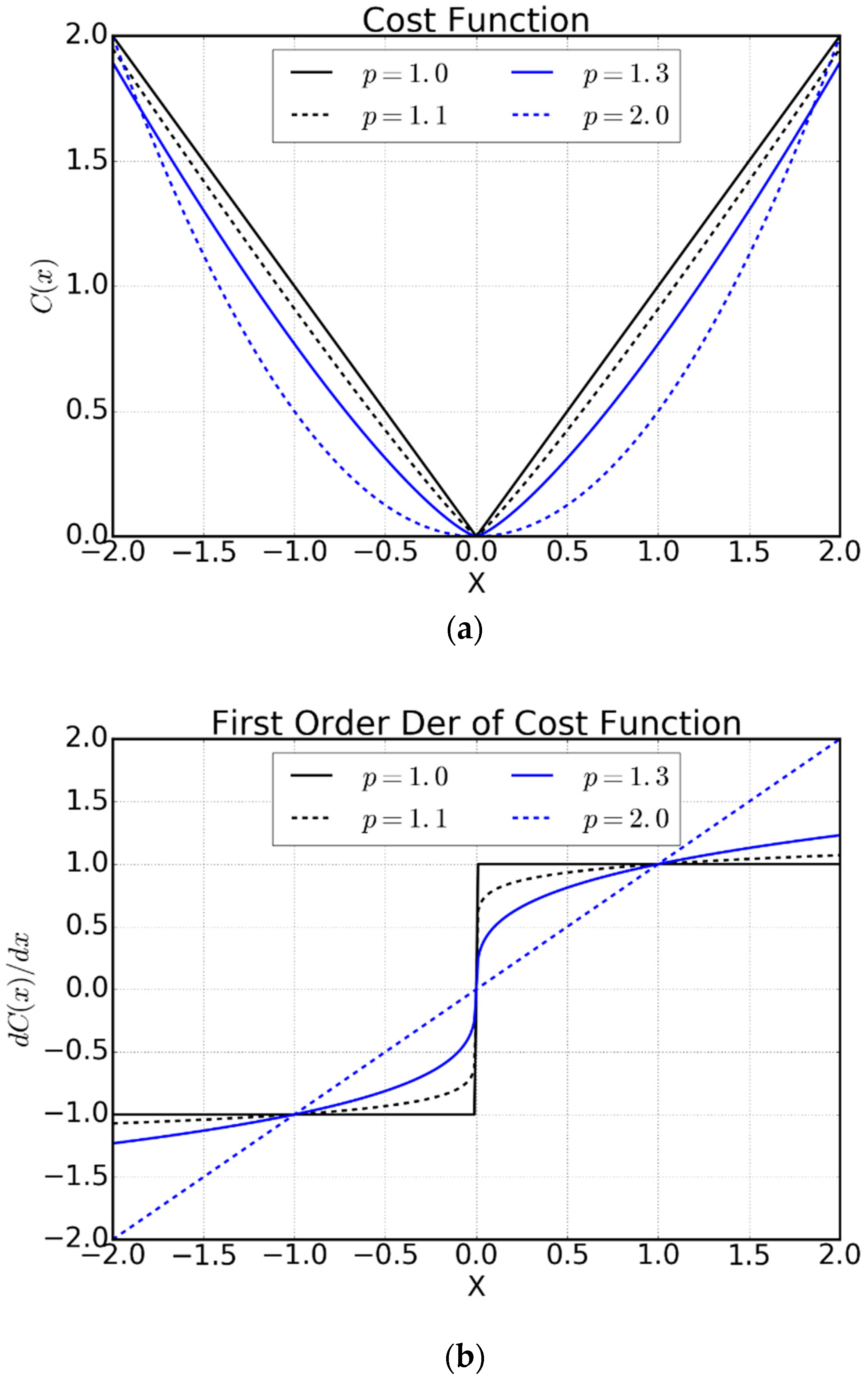
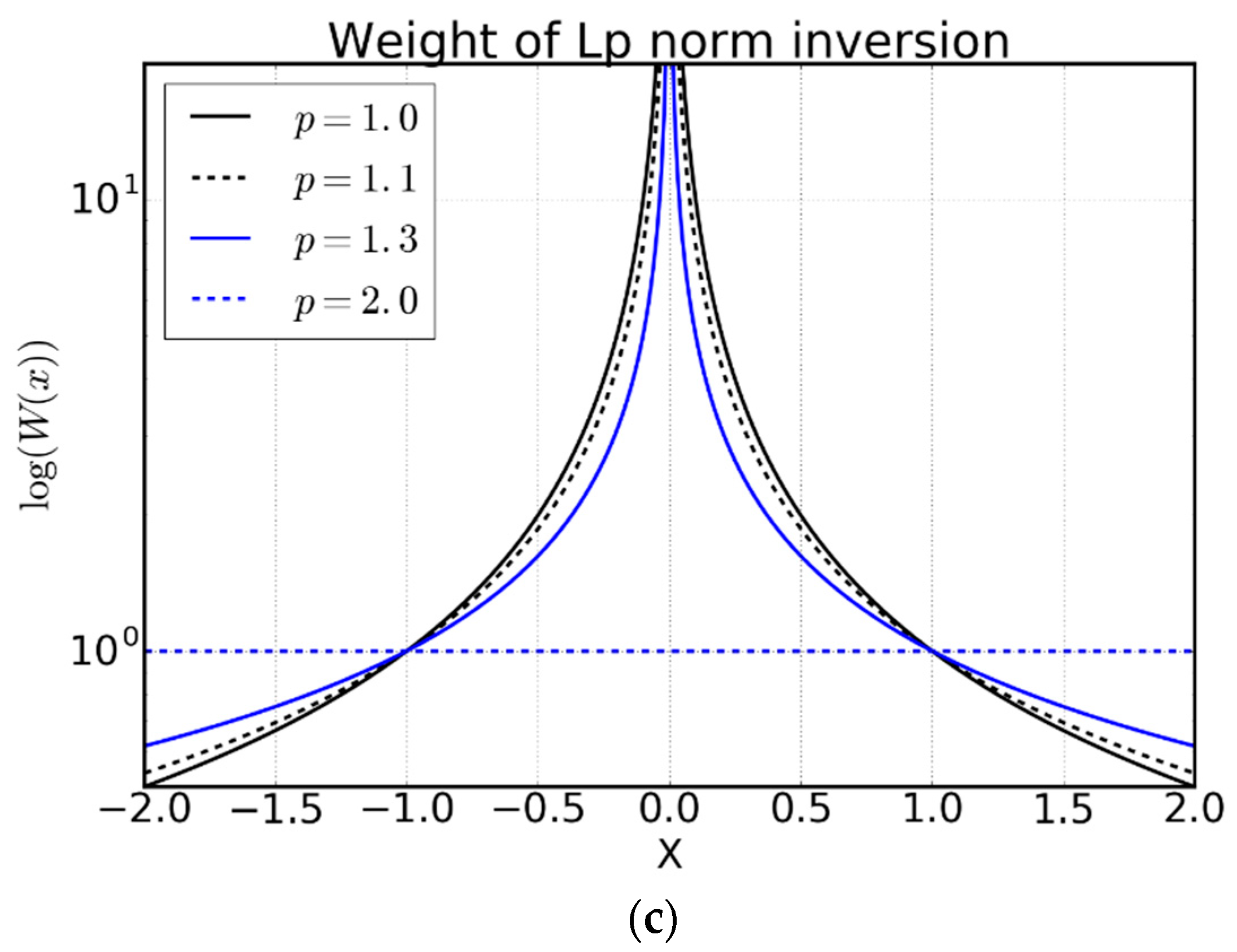
Figure 3 shows the cost functions, their first-order derivatives, and the weights for different values of p. The first-order derivative, which plays the same role as the influence function [25], needs to increase not so rapidly for large errors for the sake of robustness. From Figure 3c, we can see that as p decreases, Equation (15) puts more and more weight on the small value of residuals, the residuals of the data measurements with smaller deviations. As the errors of data measurements increase, for small values of p, the weight decreases quickly, therefore reducing their impact on the inversion. This is contrary to the case of p = 2, where the weight is one.

As an example for demonstrating the effectiveness of $L_p$ norm ($p<2$)-based optimization for suppressing the impact of input data with markedly large errors, we show below a typical geophysical problem, the inversion of seismic wave velocity from travel time picks.

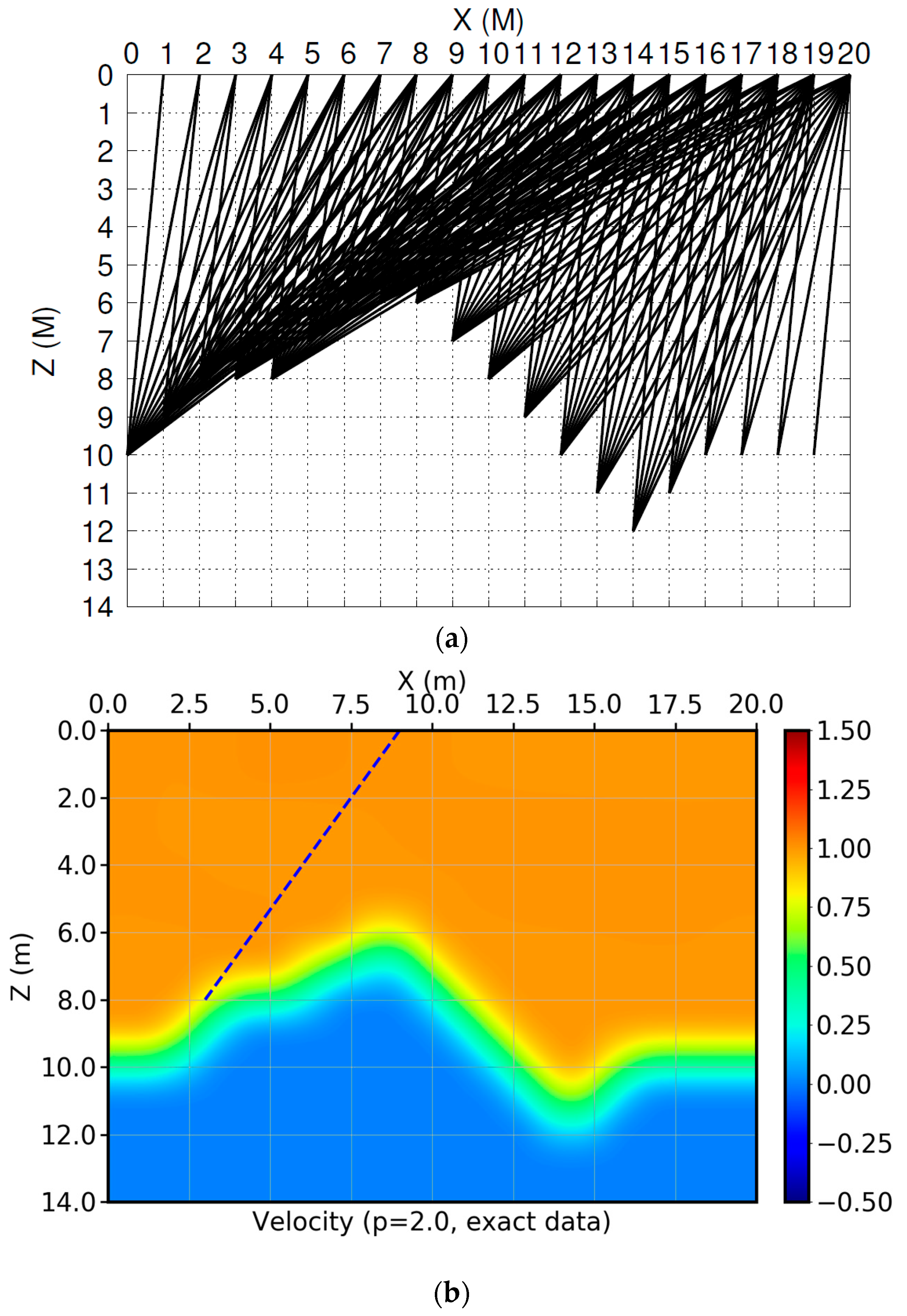
Figure 4a below shows a simple model and travel time acquisition patterns. The seismic velocity in this model is homogeneous with the exact value of v = 1 m/s. The source points are located on a horizon in the model. The receivers are distributed along the surface at z = 0 m. The solid black lines from a source to a receiver point are rays. Since the velocity model is homogeneous, the rays are straight lines. The time between each source-receiver pair is picked. The inverse problem is to invert the distribution of seismic velocity in each cell of the discretized model, and it can be formulated as

$$Av=t$$

(19)

where $t={\left(t_1,t_2,\cdots ,t_M\right)}^T$ is a column vector of travel time picks of $M$ source-receiver pairs, $v={\left(v_1,v_2,\cdots ,v_N\right)}^T$ is a column vector of the velocity in the $N$ grid cells. Each element $A_{ij}$ of $A=\left(A_{ij}\right)$ is the length of the ray segment passing through cell $j$ along ray $i$.

By carefully investigating the ray distributions in Figure 4a, we can see that the density of ray coverages is not uniform and some of the cells have no rays passing through (null space. See [19]). In the middle of the model, the ray coverage is quite dense, while on the edges, they are very sparse. This nonuniform spatial coverage is similar to the ending effect of the NMR data measurements.

When certain measurements ${\tilde{t}}_i$ are exceptionally larger or smaller (outliers) than other travel times, such as the travel time picks along the blue ray below, we expect the inversion itself can mitigate the impacts of these picks and rely more on the normal travel time.

Below, Figure 4b is the inverted result using $L_2$ norm inversion. The inputs are exact data. The inverted seismic velocity model is very close to the exact model.

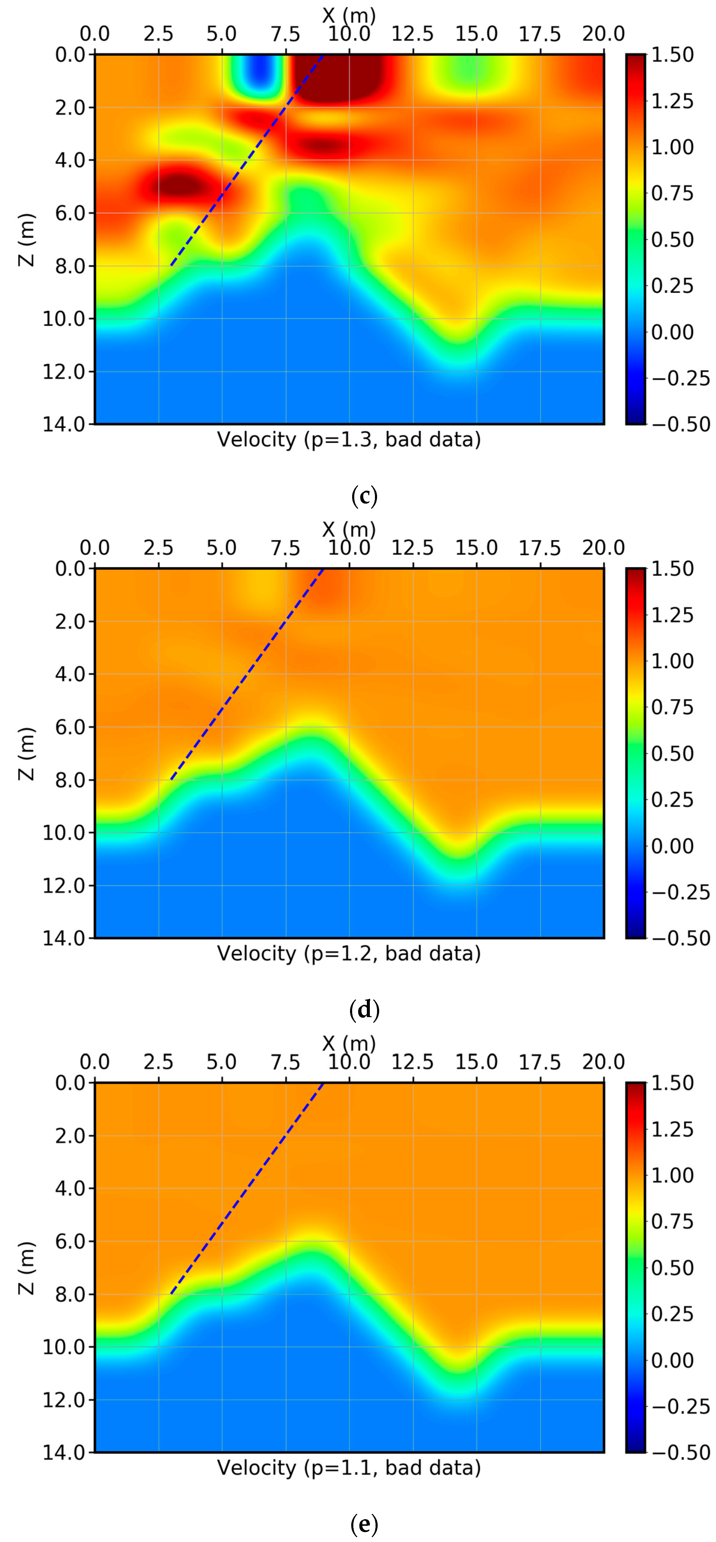
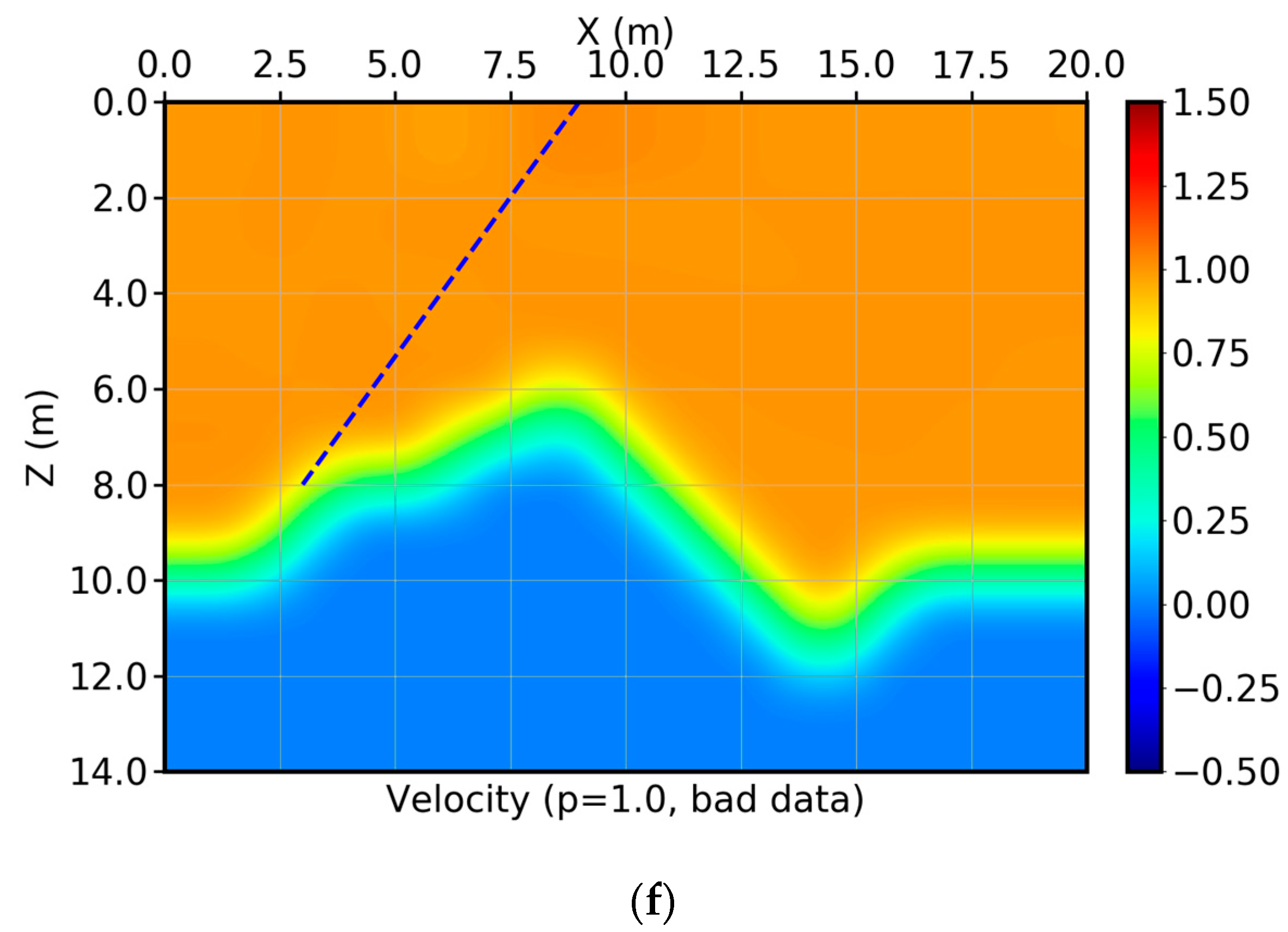
We now add a large error to the travel time pick along the ray shown with the blue line. The exact travel time is 10 s. The actual value is 20 s assuming that some systematic errors occurred to the measurements or during pre-processing. Obviously, this noise is a spatial spike and does not follow the Gaussian distribution. Different values of $p$ are used to invert this set of inputs. From Figure 4c–f, the values of $p$ are p = 1.3, p = 1.2, p = 1.1, and p = 1.0, respectively. For p = 1.1 and p = 1.0, the inverted results are both very close to the exact model. As the p increases, the inversion deteriorates. The impact of the picks with large errors is not linearly related to the changing values of p. For p = 1.2, the impact of the wrong pick starts to show its negative impact, although the impact is still restricted to the neighboring cells of that ray. For p = 1.3, the results are beyond what can be recognized. By properly reducing the value of p, the IRLS algorithm (iterative reweighted least squares, next section) can successfully recover the velocity values of all the cells with non-zero ray segments, regardless of the density of rays in that cell.

This simple model (homogeneous model, straight rays, and only one exceptional pick) shows that, for inversion using field data, $L_p$ norm inversion with p close to 1, is always safer than $L_2$ inversion. By using the $L_p$ norm with the IRLS scheme, we can recover the true physical and meaningful values of the velocity distribution even in the case of picks with nonuniform coverage and large errors.

4. Numerical Procedures

Based on the discussions in the previous sections, we illustrate the following numerical workflows for the inversion of fluid content from NMR measurements of whole cores.

Finding the optimal solution of the $L_p$ norm ($p<2$)-based optimization (9) can be achieved by applying the weight in Equation (16), followed by finding the solution to Equation (15). The procedure is iterative reweighted least squares [26]. The keyword “iterative” reflects the nature of the algorithm that the current weight (16) is dependent on the previous solution. There are a number of numerical algorithms that have been designed to solve Equation (15). Among them, least squares with QR-factorization (LSQR) [27] and conjugate gradient for least squares (CGLS) problems [28] have both been proven to be efficient and convergent. Their implementations are also straightforward. We will use the CGLS algorithm in this paper.

Three numerical procedures need to be implemented: CGLS for solving Equation (13), IRLS for solving the weighted system (15) of the L_p-norm optimization (9), and inversion conditioning. The CGLS procedure is used in the IRLS during each iteration. In each of the following workflows, we assume $A$ is a $M\times N$ matrix, $m$ is a column vector with $N$ elements, and $d$ is a column vector with $M$ elements.

The CGLS procedure for solving the linear equation $Am=d$ is given as follows:

• Choose $m_0$. Set $s_0=d-A{m}_0$, $r_0=p_0=A^T\left(d-A{m}_0\right)=A^T{s}_0$, $q_0=A{p}_0$;

• Repeat the following steps until the solution $m_k$ does not change or $k$ reaches an upper limit:
  • ${\alpha }_{k+1}=\frac{\left(r_k,r_k\right)}{\left(q_k,q_k\right)}$;
  • $m_{k+1}=m_k+{\alpha }_{k+1}{p}_k$;
  • $s_{k+1}=s_k-{\alpha }_{k+1}{q}_k$;
  • $r_{k+1}=A^T{s}_{k+1}$;
  • ${\beta }_{k+1}=\frac{\left(r_{k+1},r_{k+1}\right)}{\left(r_k,r_k\right)}$;
  • $p_{k+1}=r_{k+1}+{\beta }_{k+1}{p}_k$;
  • $q_{k+1}=A{p}_{k+1}$.

The IRLS workflow for the $L_p$ norm optimization problem for linear equation $Am=d$ is illustrated below:

• Choose $m_0$ and a small positive number $\epsilon$;

• Repeat the following steps until the solution converges:

• $r_i=d_i-{\displaystyle \sum _{j=1}^N{A}_{ij}{m}_j}$, $i=1,\cdots ,M$;

• Compute the weights for, $W_i=\{\begin{array}{ccc}{\left|r_i\right|}^{p-2}& ,& \left|r_i\right|>\epsilon \\ {\epsilon }^{p-2}& ,& \left|r_i\right|\le \epsilon \end{array}$, $i=1,\cdots ,M$;

• Apply the weights to the data, $z_i=W_i{d}_i$, $i=1,\cdots ,M$;

• Apply the weights to the linear matrix, $B=\sqrt{W}A$;

• Solve the new equation $Bm=z$ using CGLS.

There are two loops in the IRLS algorithm. The inner loop is inside the CGLS for solving linear equations as an L₂ norm problem. The outer loop is for the computation of the new matrix $B$ and the new data vector $z$ from $A$ and $d$ based on the current model estimation. It is this automatic updating for the equations that make IRLS immune to the impact of the data measurements with large errors.

Lastly, the inversion conditioning is implemented as a non-stationary smoothing operator [15,29] and applied after the IRLS workflow. The smoothing operation can also be implemented by adding the regularization term to the original cost function (9).

5. Inversion of Fluid Content from Field NMR Measurements and Error Assessments

In this section, we apply the robust inversion scheme developed in previous sections on the inversion of fluid contents from NMR measurements. We will also discuss the application of L_p-norm inversion on the data without complete quality control, and we demonstrate that the errors of the inverted parameters are localized during L_p-norm inversion.

We first measure the response map of the coil using the dual equation of (5). After calibration, the result is shown in Figure 5. The spacing between two sampling points is 1 in, the same resolution as that of the fluid content samples. Note that the response function is not homogeneous within the entire coil. This reflects the impacts of the limited size of the coil on the magnetic field, and therefore, produces negative impacts on the measurements of NMR data that must be removed during fluid content inversion.

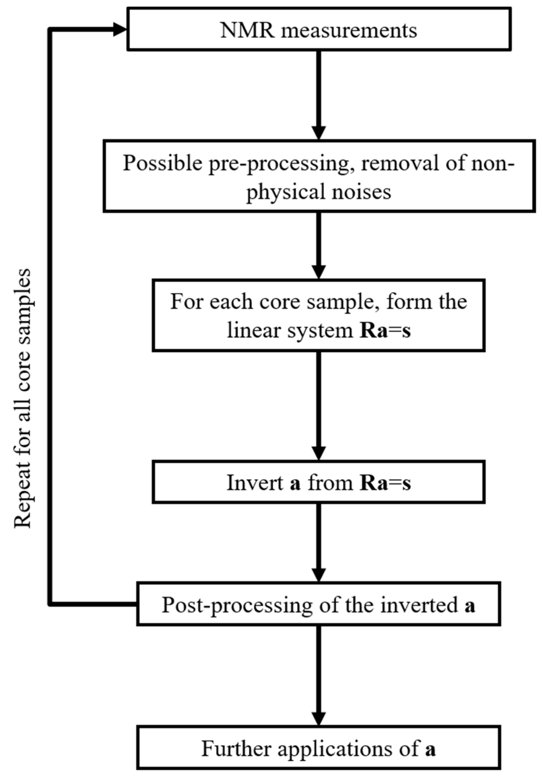
After obtaining the response map, the processing and inversion are carried out by the procedures in Figure 6. If large deviations and non-physical noises can be removed in the pre-processing step, the relatively large value of p’s can be used for inversion. Once the fluid contents have been inverted, it can be used for the estimation of other more production-related parameters such as maximum producible hydrocarbon.

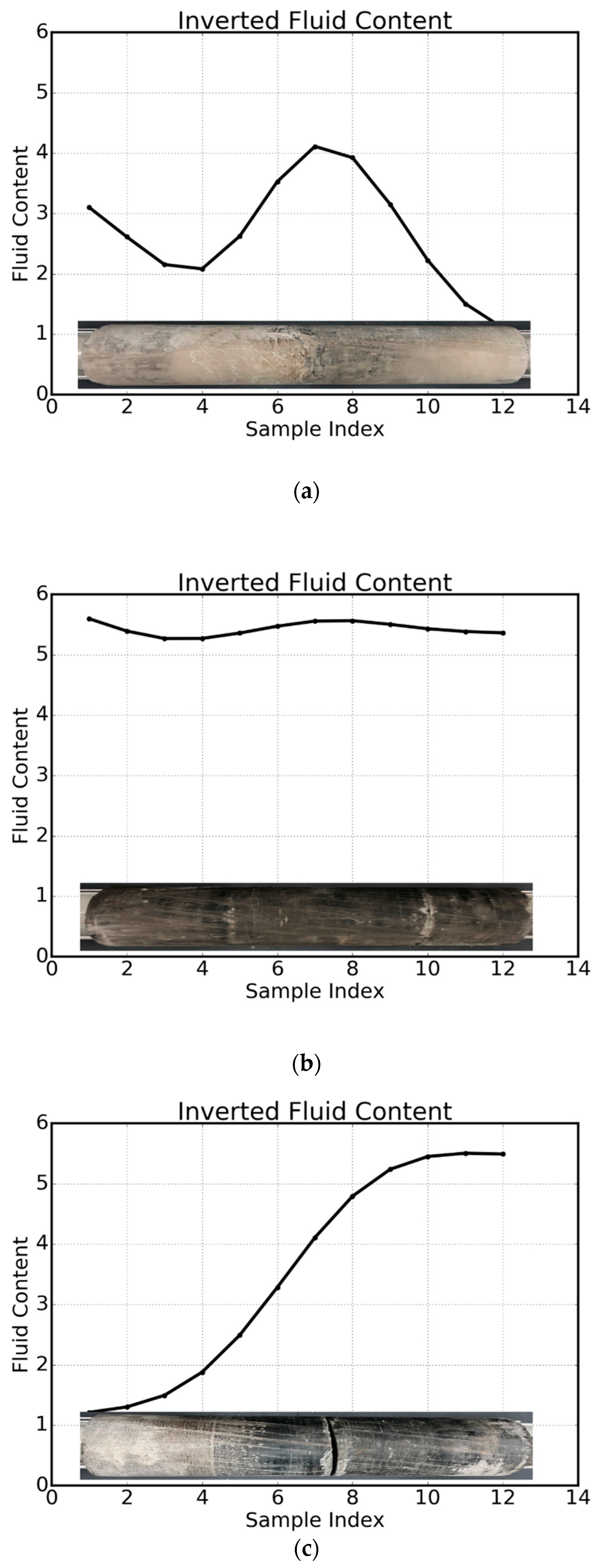
Figure 7 shows the inversion of three cores. We plot the inverted results of the fluid content and also insert the core photos. The color of the core represents the laminated distribution of kerogen along the core, a key factor for the estimation of the oil and gas reserves. The darker color indicates higher kerogen content in the core. In the pre-processing step, considering the ending effects, the first two and very last NMR signals are removed for all the core measurements. We will show the inverted results without pre-processing later on.

These three cores (a–c) represent three typical scenarios. For core A (Figure 7a), the inverted fluid content varies in a complete cycle of a down-up-down pattern. This variation pattern closely follows the color changes of the core. The resolution of the inverted fluid contents is about 2 inches. The color of core B (Figure 7b) is almost constant. This fact is correctly expressed in the inverted fluid content. For core C (Figure 7c), the kerogen consistently increases along the core, and the color darkens, which is perfectly matched by the inverted fluid content.

The p values used in the inversions in Figure 7 are all 1s, and the unreliable data measurements have been removed. According to Figure 3c and Figure 4, slightly larger values of p can still be used if all the data samples follow the normal trend, which can be predicted by Equation (8).

Next, we will show that L_p-norm inversion with small p can automatically remove the impact of data points with large measurement errors and correctly recover the effective fluid contents.

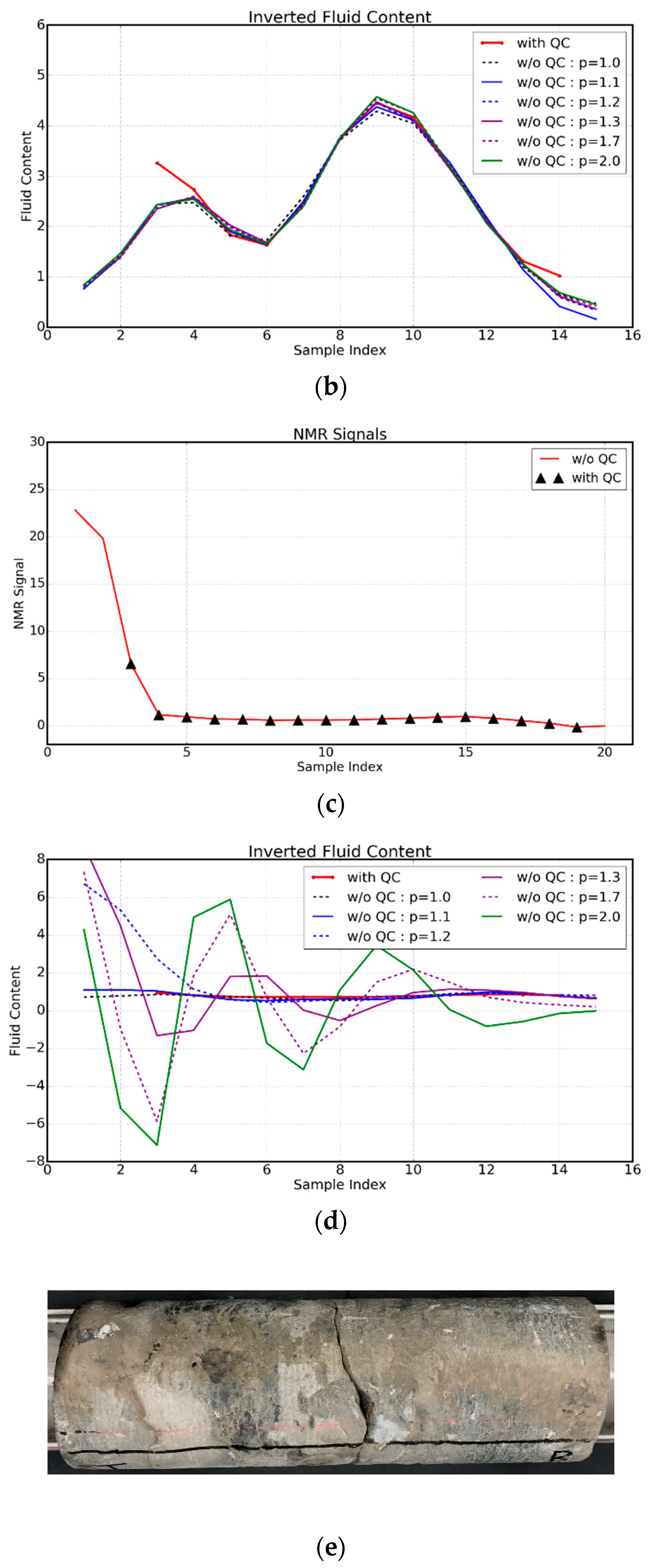
Figure 8a,c show the NMR measurements for two cores, core A and core D. Both the pre-processed (curves with triangles) and non-pre-processed (red curves) NMR data are plotted. For core A, the first two and the very last data points are negative (but with a small magnitude). For core D, the first two data points show significant deviations from the rest.

Figure 8b,d show the inverted fluid content using different values of p using the non-pre-processed data, and they are compared with those using pre-processed data (solid red curves). For core A, since the erroneous data is slightly different from the major trend, there are no large differences between the inverted results with different p’s. This indicates that for sufficiently well-prepared data, L₂ inversion shall be able to provide reasonable results.

For core D, due to the large deviations of the first two ending samples, clearly, only the results of L₁ and L₁.₁ are reasonable (The photo of core D is shown in Figure 8e). The inverted results are misleading and may result in incorrect interpretations for the fluid contents in the core and therefore lead to inaccurate calculations of oil and gas reserves.

6. Conclusions

An accurate and robust inversion method, previously developed for solving geophysical inverse problems, has been applied for the inversion of the fluid contents from the NMR measurements. This inversion allows downhole cores with arbitrary sizes compared with the detection coil, cases cannot be handled in conventional methods. Inversion based on the L_p norm can overcome the negative impacts of the heterogeneities at the ends of the magnetic field and can accurately estimate the fluid contents in cores. Spatial conditioning is an important step for the extraction of the desired information containing true physics. By properly conditioning the inverted results, the impact of the noises generated during data collection can be mitigated or removed. The inverted results show perfect matching between the fluid content and the lamination due to kerogen content in the cores.

As an important application, the high accuracy and robustness of the proposed inversion scheme make it possible to estimate the maximum producible hydrocarbon in unconventional resources, which can be obtained by subtracting the remaining fluid in preserved cores from the total fluid in the downhole logging results.