Abstract
A detailed study is undertaken of the computational modelling of a sub-platform for floating offshore wind using the software Star-CCM+ with the application of the RANS approach. First, a mathematical introduction to the governing equations is carried out. Then, the computational grid is defined, and the grid-independence of the solution is verified. A time-dependent study is performed with the selected time-step. Finally, two examples of 3D decay tests in heave of the sub-platform without and with moorings are presented, accompanied by a damping factor study, with the aim of providing a better understanding of the hydrodynamic damping of the platform. Throughout the process, three degrees of freedom (DoFs) are locked due to the limitations imposed by the use of a symmetry plane; this implementation allowed us to reduce the computational cost of each simulation by 50%. Therefore, three DoFs (heave, surge and pitch) are considered. The coupling study, adding a mooring system in the decay tests and the regular wave tests, shows good agreement between the experimental and computational results. The first half-period of the simulations presents a greater discrepancy due to the fact that the damping of the platform is lower in the computational simulation. However, this does not imply that the hydrodynamic damping is underestimated but may be directly related to the lock of various DoFs associated with the hydrodynamic damping.
1. Introduction
Reducing carbon emissions is one of the main challenges that the world must face. This is reflected in the announcements that several governments have made to go carbon neutral in the next few decades [1]. One of the most popular ways to achieve this is the electrification [2] of all the energy sectors. This creates a unique scenario for renewable technologies, which are one of the most important protagonists of this transition.
Among renewable technologies, wind energy has shown its maturity and continuous evolution, with an increase in the size of turbines [3] and expansion from onshore to offshore. Furthermore, in recent years, this transition has reached deeper areas, paving the way for floating systems to exploit a larger, and better-quality, resource while having fewer social impacts [4]. Despite this expansion, floating wind technology has some challenges that must be addressed to optimize its functioning.
Offshore wind turbines are larger and more powerful than their onshore counterparts [5]. However, floating offshore wind systems, composed of the wind turbine, the floating sub-structure and the mooring lines, have a complex behaviour, as they are affected by environmental, aerodynamic, hydrodynamic, and mooring loads. This complexity is reflected in the turbine working at sub-optimal angles and in constant oscillation and movement. In pursuit of a better performance of these systems, several concepts of floating platforms have been developed, such as spar buoys [6,7], semi-submersible platforms [8] and tension leg platforms (TLP) [9], among others.
To study the design and behaviour of these systems, several approaches exist, which are reflected in different software packages [10]. Numerical simulations are used to design these floating sub-structures and reduce the total cost of the installation of this type of structures due to their complexity. Software packages that combine strip theory and panel methods are well-known in the industry, e.g., Orca Flex [11] and FAST [12], but they present some limitations due to their neglect of viscous effects [13,14].
Another approach, which is gaining popularity in recent years due to the increase in computational power, is to apply high-fidelity numerical models such as Computational Fluid Dynamics (CFD), which combined with six degrees of freedom (6DoFs) present accurate solutions that only require the geometry and the mass properties of the platforms. These numerical models, based on the Reynolds-Averaged Navier–Stokes (RANS) equations, are used to overcome the problem of the viscous effects [15]. Some researchers have compared both approaches [8,13], achieving good agreement between both methods. It is important to highlight that there are more approaches in CFD, such as Direct Numerical Simulations (DNS), which directly apply the Navier–Stokes equations. However, this approach is very computationally expensive, and it is mainly done in academia. Another approach for turbulent modelling is the Large Eddy Simulation (LES) approach, which resolves the large-scale turbulence while modelling the small isotropic turbulent scales. For this article, the RANS approach has been used due to its maturity and its good computational cost in relation to the accuracy of the method, besides its very strong performance coupled with the maturity of the turbulent models developed around this approach. Along these lines, comparisons of different approaches for the simulation of a numerical wave flume have been done to have a better understanding of how different types of turbulence modelling could affect the behaviour of regular waves and the reflection process due to the existence of an extinction system [16].
The first studies that were carried out around CFD simulations were focused on cylindrical floaters [17]. In recent years, more complex simulations have been carried out to better understand the behaviour of these types of structures. For example, numerous articles have been published simulating different decay tests of different structures. Furthermore, another way to study these structures has been to focus on the aerodynamics of the turbine when having a defined motion in the platform [18,19,20]. Moreover, the study of this type of platforms has been extended in recent years, with several studies focused on decay testing for different degrees of freedom [11,21]. Tran et al. [19,22] studied the unsteady aerodynamics of a turbine by imposing a sine function onto a spar platform. In recent years, various articles have been focusing on the complex behaviour of these structures. Liu et al. [22] studied the effects of the movement of the OC4 DeepCWind platform on the aerodynamics of the wind turbine and vice versa [23], work that continued with the development of an aero-hydro-mooring elastic fully coupled tool by inducing a combined wind and wave condition.
Following their work, Tran and Kim [22] investigated a 5MW wind turbine over an OC4 DeepCWind semi-submersible platform by comparing the results of the dynamic fluid body interaction methodology with those obtained with the open-source software FAST. The aero-hydrodynamic performance of the system was studied under coupled wind-wave conditions and in decay testing [24]. Study of the IDEOL platform in regular wave tests by applying a coupled simulation of multi-body systems with CFD and comparison of the results with experimental data was done by Beyer et al. [25]. An unsteady actuator line model for the aerodynamic simulation coupled with a CFD solver for the hydrodynamic part was studied by Cheng et al. [26].
Similar works have been done for floating structures but for different aims. Bi et al. [27] present a work in which they experimentally study the decay testing of a multi-module aquaculture platform where they analysed the motion of the platform while also analysing, apart from calculating the natural periods, the stiffness with the mooring system. Furthermore, they study the response of the platform when facing regular waves. In relation to the experimental study of mooring systems in this type of structures, Zhao et al. [28] carried out deep research on this topic. Finally, joint research of computational and experimental approaches has been done too around this type of structures, focusing on extreme conditions [29].
However, it is important to find a computational mesh that has a good relation between computational cost and accuracy. The latter one is especially important, since a bad mesh can modify the response of the sub-platform analysed.
This work presents in the following section a summary of the mathematical treatment used in this type of problems. Furthermore, the procedure followed in order to obtain the results is defined, to give a better understanding of this research. Finally, Section 3 presents the outputs of the simulations for platforms both with and without moorings, validated through the data obtained by Saitec Offshore Technologies in their experiments in the LIR/NOTF laboratory through the ARCWIND Project (adaptation and implementation of floating wind energy conversion technology for the Atlantic region).
2. Materials and Methods
2.1. Governing Equations
The behaviour of every incompressible Newtonian flow can be described with the mass and momentum conservation equations, Equations (1) and (2), respectively. These equations are Navier–Stokes equations.
where i and j are the indexes for 2D flows, ui is the time-averaged component of the velocity vector, ρ is the density of the fluid, t the time, p the pressure, g the gravity acceleration and τij the viscous stress tensor. However, transfer of these equations to computational modelling is not extended due to the high computational cost. Therefore, all the instant values obtained in the Navier–Stokes equations are decomposed in mean and fluctuating values with the Reynolds decomposition once we apply Reynolds-Averaged Navier–Stokes (RANS), Equations (3) and (4).
where U represents the flow velocity, Ug is the velocity of the grid nodes, pd is the dynamic pressure by substracting the hydrostatic component from the total pressure p, and g is the gravity acceleration, ρ is the mixture density of both flows, μ is the effective dynamic viscosity, ν is the kinematic viscosity and νt the eddy kinematic viscosity.
With this decomposition, an introduction of new terms appears, creating an open system of equations. Thus, more equations are needed to close them. In this scenario, different turbulence models have been developed throughout the years to solve this problem. To do that, these models associate the Reynolds stresses with the mean flow variables. In this study, the k-ω SST turbulence model, Equations (5) and (6), developed by Menter is used [30].
where k is the turbulence kinetic energy, u is the velocity of the flow, ω is the specific dissipation rate, and ν is the kinematic viscosity, while σ, β and a are constants.
However, in this type of problems, more than one fluid is normally simulated, and another tool is needed for the definition of each fluid and for tracking the free surface. In this study, for this aim, the Volume of Fluid (VOF) presented by Hirt and Nichols [31] is used. It is a free-surface modelling technique, i.e., a numerical technique for tracking and locating the free surface (or fluid–fluid interface). For each phase considered in the model, a variable is introduced as the volume fraction of the phase in the computational cell. Volume fractions represent the space occupied by each phase, and the laws of conservation of mass and momentum are satisfied by each phase individually. In each of the control volumes, the volume fractions of all phases sum up to unity. This model defines the percentage of volume of a certain cell that is occupied by a fluid. This percentage is defined by the following variable:
where αi is the variable, Vi the volume occupied by the specified fluid and V the volume of the cell. In FOWT simulations, fluids are defined by primary and secondary fluids, which have an index of 1 and 0, respectively. So, when a cell is occupied only with the primary fluid, in this case water, its value will be one, and when only air exists, the value will be zero, and finally when the cell has both fluids, a fraction between 0 and 1 will determine the ratio of volume between them. The α-function behaves as another property of the fluid. Because of that, it satisfies the advection equation [32], which states that the material volumes stay constant along the streamlines:
The position of the free surface corresponds to the value α = 0.5, while the physical properties of each fluid and their volume fraction are given by [33]:
where ρi is the specific density of each fluid and μi its viscosity. The position of the free surface in the cell is calculated by imposing a perpendicular line to the maximum descent gradient to the cells in its proximity.
2.2. Mesh
2.2.1. Mesh Domain
The computational domain is a semi-cylinder with a diameter of 5 times the hydrodynamic diameter of the platform (DH) and a height of 10 times the height of the device. These dimensions are sufficiently large to avoid the effect of wave reflection due to the curved walls while maintaining the same depth as the one used in the experimental runs. The volume is differentiated in two main meshes. The background mesh, which embraces the whole volume of study, and the overset mesh, which is focused on the movement of the platform and the behaviour of the fluid alongside it, has variable cell size depending on the area covered.
In the background mesh, five different areas can be distinguished. In four of them, the cell size is defined using the trimmer anisotropic function, which allows us to modify the cell dimensions in all three axes. The area where the cells are not modified is that corresponding to the air, the one that is not numbered in Figure 1, and that is because it is the least important area for this analysis; therefore, it has the largest cells of the volume of study.
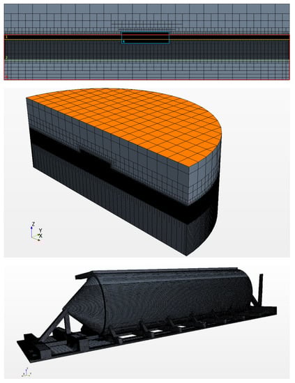
Figure 1.
Section with the different sub-volumes used in the background mesh (top) and the general volume of study (mid) and details of the geometry simulated (bottom).
The other 4 areas are defined to have a better understanding of them. Area 1 is the free surface area, which has the smallest cells of the background mesh. The cells’ area is defined considering the wavelength, obtained by the heave natural period of the platform, and then the Z dimension is defined by using an aspect ratio (AR) of 4, which is defined in Equation (11). Both horizontal axes, x and y, have the same dimensions in the whole volume.
Area 2, the under-free-surface refinement space, is refined to not lose energy of the waves in that area formed due to the movement of the platform. The AR is maintained in all volumes. The length of its cells in the x and y axes is twice that in the free surface.
The deep-water area, Area 3 in Figure 1, has the same size in the horizontal axes as the air area. The last zone, called the column and defined as Area 4, has the same cell size as the free surface one. This area is created to optimize the data transfer between the overset mesh and the background mesh, and to try to avoid any problems in the mesh definition due to cell size differentiation, which could lead to the breaking of the simulation.
In the background mesh, three types of boundaries can be identified. The top of the volume (the orange face in Figure 1) is defined as a pressure outlet area, which allows the air to flow freely. The curved and bottom boundaries are defined as walls with a non-slip condition, while the vertical boundary in the XZ plane is defined as a symmetry plane, which allows us to only study half of the platform.
This last boundary has an important effect in the reduction of the computational cost of the simulations. However, it only allows us to study three degrees of freedom (DoFs), namely, heave, surge and pitch.
The overset mesh has two different areas: the free surface area, which is designed to cover the free surface interacting with the platform, and the background. Due to this, the free surface area of the overset mesh will be higher than the free surface area of the background mesh. On the contrary, the cell size of it will be much smaller, with its dimensions being 60% smaller than those of the free surface area of the background mesh. The rest of the overset has the same cell size as the cells in Area 4 of the background mesh. Moreover, a prism layer condition is applied around the platform. With a total width of 5 mm and 13 layers with a growth coefficient of 1.2, it ensures that we do not have a value of wall y+ higher than 1.5.
2.2.2. Mesh Independence Study
A mesh convergence study is needed to understand how the mesh definition affects the response of the platform in the different tests, and to achieve the best possible ratio between definition and computational cost. To achieve this aim, 3 grids were designed to compare their results in one of the cases. A decrease in all the dimensions of 50% was presented to know how the response was sensitive to the cell size change. The free surface cells, the smallest ones of the tank mesh, are 50, 100 and 200 times smaller in relation to the height of the device. The overset cells have a height between 50% and 70% of the free surface cell, depending on each of the grids. Thus, 3 grids of clearly different computational weights were obtained, which can be seen in Table 1.

Table 1.
Number of total cells for each of the grids considered in the mesh convergence study.
All the grids have been simulated with the same time-step to focus just on the dependency of the cell size. In Figure 2, it can be seen that there is almost no difference between the 3 grids. However, some tendencies can be seen when analysing the damping ratios of the signals.
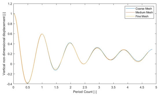
Figure 2.
Direct comparison of the signals obtained in the mesh sensitivity study.
The damping ratios can be observed by comparing the mean amplitudes of each of the periods and the decrease in amplitude that can be seen in the period itself. This method is the same as that which Li and Bachinsky-Polic have used [34]. To do that, different equations are needed. The decrease in amplitudes is compared logarithmically:
where ηi is the peak or drought of the decay signal. It is always compared in intervals of 2 to have a comparison between continuous peaks or droughts. The value used as a decrease in the peak or drought value is then used to calculate the damping ratio in that period [31].
Then, to compare the results obtained from this mesh dependency study, the tendency of the points has been defined. A comparison of linear, quadratic and cubic tendencies has been done to see if the highest complexity of the curve has a relationship with the degrees of freedom unlocked.
The damping ratios calculated for each of the meshes in the size dependency study can be seen in Figure 3. In it, the different fittings are set to see how each mesh compare to the other two. The different fittings show that similarities between the two finest meshes increase when the grade of the fitting increases. The most similar fittings are when the grade of the fitting is the same as the degrees of freedom unlock in the simulations.
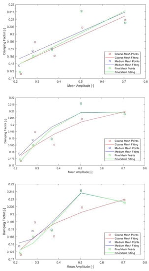
Figure 3.
Comparison of the relation of the tendencies used for the case with linear (up), quadratic (mid) and cubic (down) fitting.
Besides the mesh sensitivity study, a time-step dependency study was run to see which time-step in relation to the period was needed. The first step of this process was to calculate the Courant number to ensure that all time-steps considered were good enough theoretically. It arises in the numerical analysis of explicit time integration schemes, when these are used for the numerical solution. As a consequence, the time-step must be less than a certain time in many explicit time-marching computer simulations; otherwise the simulation produces incorrect results.
This can be seen in Table 2 in which for the three time-steps considered, and the cell size, all the possible Courant numbers in each of the meshes were reasonable. These 3 values are TN/1000, TN/1800 and TN/3200, being TN the natural period of the degree of freedom analysed. All the values are low, reinforcing the idea of the use of these time-steps, which ensure that the platform will not move more than the height of the smallest cell of the background mesh. In this study, the heave natural period was used. This was done because the natural period of heave is smaller than the other degrees of freedom used in this study.
Table 2.
Courant number for every combination of the mesh convergence study.
With this aspect, all the cells, at least, have quality considering the wave celerity and the time-steps of the study. A comparison of the signals obtained in heave motion is presented to see how, with the same starting conditions.
A total of 9 cases were considered in the mesh convergence study. This is the number obtained by combining the 3 grids and 3 time-steps. To see the quality of the general mesh, the Courant number is calculated for each of the meshes. Although there are 9 cases, the time dependency study was carried out in Grid 2, also known as the medium grid.
In Figure 4a small variance in the period of the decay can be seen, although it seems to not affect the amplitudes of the signals.
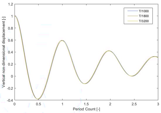
Figure 4.
Signal comparison of the different time-steps used in the time dependency study.
Figure 5 shows that the differences in the signals are more significant in the latter periods, which shows that the sensibility of the sub-platform movement is greater at lower velocities.
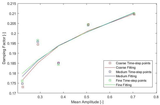
Figure 5.
Cubic fitting for the time dependency study where all the time-steps showed similar behaviour with increased differences in the latter periods.
Once the sensitivity study was finished, we decided to use the medium grid and the time-step TN/1800 to obtain the most accurate results possible while keeping the computational cost as low as possible.
3. Results and Discussion
3.1. Decay Tests without Moorings
The first study was to simulate the decay test of the platform in heave without any external forces, such as moorings, that could affect the behaviour of the tests. In the computational runs, only three DoFs are unlocked, surge, heave and pitch, while the rest are locked. This is done due to the symmetry plane imposed in all the simulations to reduce the computational cost of each of the runs.
The first step is to compare the results of the experimental and computational runs over time. To do this, the numerical platform is positioned at the highest point recorded by the experimental runs and then it is allowed to fall, and both signals are compared from their highest point recorded.
In Figure 6, this comparison can be seen clearly. Both signals oscillate around the same equilibrium height, which is a good indication. However, it is clear that the computational run has a lower hydrodynamic damping, as expected. Moreover, the value is similar in the first ones, but starts varying in the latter one. Again, this may be due to the existence of different numbers of DoFs.
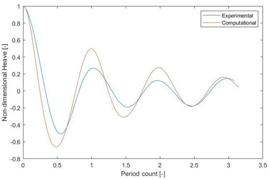
Figure 6.
Signal comparison of the experimental (blue) and computational (orange) decays without the interaction of mooring systems.
However, to have a better understanding of the run, a damping factor study was undertaken. Because of the difference of DoFs in each of the tests, only a linear fitting was done to compare the damping of each of the tests. The slopes of each of the fittings can be related to the damping of each of the experiments. The slope of the experiment is 0.11, while the slope of the numerical fitting is 0.03. Clearly, the damping in the experimental campaign is much higher.
In Figure 7, it can be seen that the damping factor in the latter period is 0, which means that the amplitude increased in the experimental runs.
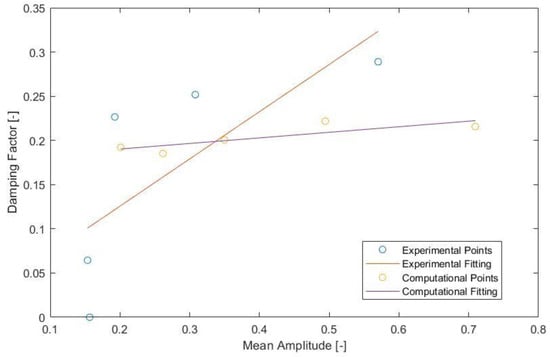
Figure 7.
Damping factor study between the experimental and computational tests with linear fitting of both. Larger degree fittings were not studied due to the different DoFs used in both runs.
This is because the amplitudes are very low and the behaviour of the platform in other DoFs that were not modelled in the simulations affects the response in heave. This is very difficult to simulate in the computational domain, and impossible if some DoFs are locked. These results magnify the effect of the damping in the platform, creating a larger slope. Although in the comparison the computational data seem to follow a linear tendency, it is important to remember that a cubic fitting adapts much better to its results, due to the three DoFs used in the runs. However, the different numbers of DoFs between the experimental and computational runs make this fitting less interesting.
Figure 8 shows this by deleting the last two damping factors, related to the last period, which show a clearer relation between the slopes, where the experimental test gives a slope of 0.0467 while the numerical one has a slope of the value 0.0287. The difference in height is, again, given by the lesser damping in the numerical models; however, the relation between periods is more logical. This makes it clear that for further research, a much longer time of decay testing will be needed, apart from the study of different DoFs.
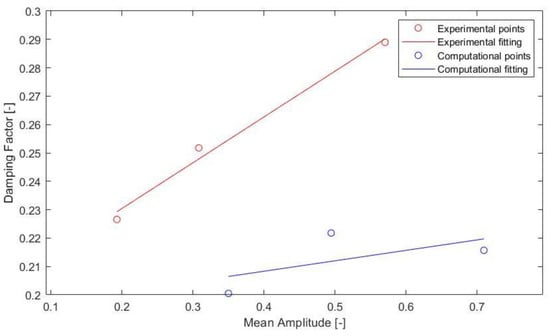
Figure 8.
Damping factor comparison with the data from the first periods in order to delete the more significant effect of DoFs that were not unlocked in the computational tests.
3.2. Decay Test with Moorings
To have more data to compare and to test the quality of the meshes, a decay test with mooring lines was performed. This gives us the possibility to, once again, comparing our simulations with the experimental tests and also to testing the same uncertainty with different numbers of DoFs active but with lower impact due to the existence of the mooring lines.
Thanks to the mooring lines behaving symmetrically as springs for this particular set of tests, we were able to keep the symmetry plane in the computational tests. The lines are positioned with a gap of 90 degrees between them and are displaced 45 degrees to the x-axis. Moreover, the lines are parallel to the XY (horizontal) plane.
The springs are connected to the same point of the platform as in the experimental tests and to the curved wall of the volume of study in the simulations, with the sole aim of maintaining the same position in relation to the platform.
Because of the existence of the mooring lines in the experimental tests, which work to maintain the platform in the desired position, a lower effect of the DoFs that are locked in the simulations is observed, showing much better matching between the experimental and computational tests.
Figure 9 shows the comparison over time of the decay test with mooring lines, in which a closer relationship between the two lines can be clearly seen. Moreover, the experimental signal keeps decreasing in the third period, which may be related to a decrease in the influence of the effect of roll in these tests.
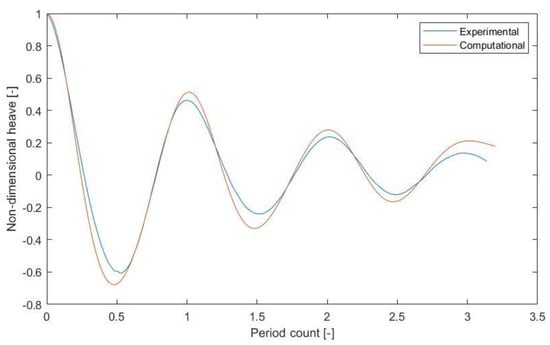
Figure 9.
Signal comparison of the experimental (blue) and computational (orange) decays with the interaction of mooring systems.
The computational signal maintains the same period throughout all the experiments, with a negligible error in the period of less than 1%, a value that can be seen in the decay tests without moorings as were shown previously in Figure 6.
The tendency for larger amplitudes in the computational runs is again reproduced. The damping factor study is done for this type of decays, showing a much better relation than in the runs without moorings.
Figure 10 shows that both fittings are much closer than in the comparisons without moorings. The slope of the experimental test is 0.0155, while that of the computational test is 0.022. This is contrary to the tendency found for the case without moorings, however, which shows less total damping because it stays below the experimental fit.
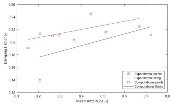
Figure 10.
Damping factor study between the experimental and computational tests with linear fitting of both.
4. Conclusions
In this article, we have focused on the process of the first steps to analyse floating platforms for offshore wind, aiming to start a whole computational simulation of the design and verification process for this type of structures. We started with mesh and time dependency studies, and then we analysed a few of the first steps needed for this type of structures, such as decay tests and regular wave tests. To be able to compare the numerical modelling, the motion obtained from experimental tests in the LIR/NOTF wave basin by Saitec Offshore Technologies was used as the ground truth.
The main aim of this study was to consolidate a good basis for both hydrodynamic and computational understanding of this type of simulations before proceeding to more complex steps such as towing tank testing including regular and irregular wave tests.
Throughout the process, three DoFs were locked due to the limitations of the use of a symmetry plane. However, this implementation allowed us to decrease the computational weight of each of the simulations is half. Because of that, only heave, surge and pitch DOFs were used. The coupling study, adding a mooring system in the decay tests and the regular wave tests, showed good relations between the experimental and computational results.
Although the results shown in the study are promising, some clear improvements can be made in future research to close the differences shown in our comparisons.
The damping in the simulations at low velocities, peaks and droughts is lower in the computational runs than in the experimental ones. This is related to the dynamic viscosity, which should vary with the movement of the platform instead of being considered constant. We believe that the difference is more visible in a platform like the studied one with a complex geometry.
The first half-period of the simulations has a greater discrepancy in time due to the damping, because in those first moments the damping of the platform is lower in the computational domain. However, this does not imply that we are underestimating the hydrodynamic damping but may be directly related to the lock of various DoFs, defining the hydrodynamic damping in those DoFs.
Although the application of the symmetry plane is commonly used for this type of research, the lock of three DoFs may be directly related to the hydrodynamic damping of the platform, which allows the researchers some margin of error.
Moreover, the existence of sensors in the experimental prototype imposes a small difference in its behaviour that cannot be simulated.
In future research, more detailed analysis will be conducted on the decay testing, and the mesh and time dependency studies will be extended to regular and irregular waves, as well as to currents and towing tests, which are of great importance for this type of structures. Finally, the simulations show promising results, and the researchers feel positive regarding the implementation of this type of simulations in industrial processes, which can be of great help when studying the behaviour of platforms taking into consideration the non-linearity with greater detail.
Author Contributions
Conceptualization, L.G.-C.; methodology, validation, G.I.; formal analysis, J.M.B. and G.I.; data treatment, L.G.-C.; writing—original draft preparation, L.G.-C.; writing—review and editing, J.M.B. and G.I.; supervision, J.M.B. and G.I. All authors have read and agreed to the published version of the manuscript.
Funding
The current investigation was developed under the framework of the European Regional Development Fund through the “Interreg Atlantic Area Programme” under contract EAPA 344/2016, providing experimental inputs to complete this study.
Institutional Review Board Statement
Not applicable.
Informed Consent Statement
Not applicable.
Data Availability Statement
Not applicable.
Acknowledgments
The authors would like to thank the University of the Basque Country through the research group (GIU19/029)-(IT1314-19) and Saitec Offshore Technologies for their valuable guidance and data provided for the validations through the ARCWIND Project (adaptation and implementation of floating wind energy conversion technology for the Atlantic region).
Conflicts of Interest
The authors declare no conflict of interest.
Abbreviations
| AR | Aspect Ratio |
| CFL | Courant–Friedrichs–Lewis number |
| DoF | Degree of Freedom |
| DR | Damping Ratio |
| FOWT | Floating Offshore Wind Turbine |
| RANS | Reynolds-Averaged Navier–Stokes |
| TLP | Tension Leg Platforms |
| VOF | Volume of Fluid |
References
- Carbon Neutral Government Programme. Available online: https://environment.govt.nz/what-government-is-doing/key-initiatives/carbon-neutral-government-programme/ (accessed on 15 June 2021).
- Jacobson, M.Z.; Delucchi, M.A.; Bauer, Z.A.F.; Goodman, S.C.; Chapman, W.E.; Cameron, M.A.; Bozonnat, C.; Chobadi, L.; Clonts, H.A.; Enevoldsen, P.; et al. 100% Clean and Renewable Wind, Water, and Sunlight All-Sector Energy Roadmaps for 139 Countries of the World. Joule 2017, 1, 108–121. [Google Scholar] [CrossRef] [Green Version]
- Serrano-González, J.; Lacal-Arántegui, R. Technological Evolution of Onshore Wind Turbines—A Market-Based Analysis. Wind Energy 2016, 19, 2171–2187. [Google Scholar] [CrossRef] [Green Version]
- Rinaldi, G.; Garcia-Teruel, A.; Jeffrey, H.; Thies, P.R.; Johanning, L. Incorporating Stochastic Operation and Maintenance Models into the Techno-Economic Analysis of Floating Offshore Wind Farms. Appl. Energy 2021, 301, 117420. [Google Scholar] [CrossRef]
- Li, H.; Guedes Soares, C.; Huang, H.-Z. Reliability Analysis of a Floating Offshore Wind Turbine Using Bayesian Networks. Ocean Eng. 2020, 217, 107827. [Google Scholar] [CrossRef]
- Tian, X.; Xiao, J.; Liu, H.; Wen, B.; Peng, Z. A Novel Dynamics Analysis Method for Spar-Type Floating Offshore Wind Turbine. China Ocean Eng. 2020, 34, 99–109. [Google Scholar] [CrossRef]
- Nematbakhsh, A.; Olinger, D.J.; Tryggvason, G. Nonlinear Simulation of a Spar Buoy Floating Wind Turbine under Extreme Ocean Conditions. J. Renew. Sustain. Energy 2014, 6, 033121. [Google Scholar] [CrossRef]
- Hu, C.; Sueyoshi, M.; Liu, C.; Liu, Y. Hydrodynamic Analysis of a Semi-Submersible Type Floating Wind Turbine. In Proceedings of the 11th (2014) Pacific/Asia Offshore Mechanics Symposium, PACOMS 2014, Shanghai, China, 12–16 October 2014; International Society of Offshore and Polar Engineers: Mountain View, CA, USA, 2014; pp. 1–6. [Google Scholar]
- Nematbakhsh, A.; Bachynski, E.E.; Gao, Z.; Moan, T. Comparison of Wave Load Effects on a TLP Wind Turbine by Using Computational Fluid Dynamics and Potential Flow Theory Approaches. Appl. Ocean Res. 2015, 53, 142–154. [Google Scholar] [CrossRef] [Green Version]
- Dunbar, A.J.; Craven, B.A.; Paterson, E.G. Development and Validation of a Tightly Coupled CFD/6-DOF Solver for Simulating Floating Offshore Wind Turbine Platforms. Ocean Eng. 2015, 110, 98–105. [Google Scholar] [CrossRef] [Green Version]
- Ocrcina OrcaFlex Manual. Available online: https://www.orcina.com/webhelp/OrcaFlex/Default.htm (accessed on 23 October 2021).
- Jonkman, J.; Buhl, M.L. FAST User Guide; National Renewable Energy Laboratory: Golden, CO, USA, 2005.
- Tran, T.T.; Kim, D.-H. The Coupled Dynamic Response Computation for a Semi-Submersible Platform of Floating Offshore Wind Turbine. J. Wind Eng. Ind. Aerodyn. 2015, 147, 104–119. [Google Scholar] [CrossRef]
- Gueydon, S.; Weller, S. Study of a Floating Foundation for Wind Turbines. J. Offshore Mech. Arct. Eng. 2013, 135, 031903. [Google Scholar] [CrossRef]
- Burmester, S.; Vaz, G.; Gueydon, S.; el Moctar, O. Investigation of a Semi-Submersible Floating Wind Turbine in Surge Decay Using CFD. Ship Technol. Res. 2020, 67, 2–14. [Google Scholar] [CrossRef]
- Galera-Calero, L.; Blanco, J.M.; Izquierdo, U.; Esteban, G.A. Performance Assessment of Three Turbulence Models Validated through an Experimental Wave Flume under Different Scenarios of Wave Generation. J. Mar. Sci. Eng. 2020, 8, 881. [Google Scholar] [CrossRef]
- Quallen, S.; Xing, T.; Carrica, P.; Li, Y.; Xu, J. CFD Simulation of a Floating Offshore Wind Turbine System Using a Quasi-Static Crowfoot Mooring-Line Model. J. Ocean Wind Energy 2014, 1, 10. [Google Scholar]
- Tran, T.T.; Kim, D.-H. A CFD Study into the Influence of Unsteady Aerodynamic Interference on Wind Turbine Surge Motion. Renew. Energy 2016, 90, 204–228. [Google Scholar] [CrossRef]
- Khosravi, M.; Sarkar, P.; Hu, H. An Experimental Investigation on the Performance and the Wake Characteristics of a Wind Turbine Subjected to Surge Motion. In 33rd Wind Energy Symposium; AIAA SciTech Forum; American Institute of Aeronautics and Astronautics: Reston, VA, USA, 2015. [Google Scholar]
- Burmester, S.; Vaz, G.; el Moctar, O. Towards Credible CFD Simulations for Floating Offshore Wind Turbines. Ocean Eng. 2020, 209, 107237. [Google Scholar] [CrossRef]
- Tran, T.; Kim, D.; Song, J. Computational Fluid Dynamic Analysis of a Floating Offshore Wind Turbine Experiencing Platform Pitching Motion. Energies 2014, 7, 5011–5026. [Google Scholar] [CrossRef]
- Liu, Y.; Xiao, Q. Development of a Fully Coupled Aero-Hydro-Mooring-Elastic Tool for Floating Offshore Wind Turbines. J. Hydrodyn. 2019, 31, 21–33. [Google Scholar] [CrossRef] [Green Version]
- Liu, Y.; Xiao, Q.; Incecik, A.; Peyrard, C.; Wan, D. Establishing a Fully Coupled CFD Analysis Tool for Floating Offshore Wind Turbines. Renew. Energy 2017, 112, 280–301. [Google Scholar] [CrossRef] [Green Version]
- Tran, T.T.; Kim, D.-H. Fully Coupled Aero-Hydrodynamic Analysis of a Semi-Submersible FOWT Using a Dynamic Fluid Body Interaction Approach. Renew. Energy 2016, 92, 244–261. [Google Scholar] [CrossRef]
- Beyer, F.; Choisnet, T.; Kretschmer, M.; Cheng, W. Coupled MBS-CFD Simulation of the IDEOL Floating Offshore Wind Turbine Foundation Compared to Wave Tank Model Test Data. In Proceeding of the Twenty-Fifth International Ocean and Polar Engineering Conference, Kona, HI, USA, 21–26 June 2015; International Society of Offshore and Polar Engineers: Kona, HI, USA, 2015. [Google Scholar]
- Cheng, P.; Huang, Y.; Wan, D. A Numerical Model for Fully Coupled Aero-Hydrodynamic Analysis of Floating Offshore Wind Turbine. Ocean Eng. 2019, 173, 183–196. [Google Scholar] [CrossRef]
- Bi, C.-W.; Ma, C.; Zhao, Y.-P.; Xin, L.-X. Physical Model Experimental Study on the Motion Responses of a Multi-Module Aquaculture Platform. Ocean Eng. 2021, 239, 109862. [Google Scholar] [CrossRef]
- Zhao, Y.; Guan, C.; Bi, C.; Liu, H.; Cui, Y. Experimental Investigations on Hydrodynamic Responses of a Semi-Submersible Offshore Fish Farm in Waves. J. Mar. Sci. Eng. 2019, 7, 238. [Google Scholar] [CrossRef] [Green Version]
- Liu, H.-F.; Bi, C.-W.; Zhao, Y.-P. Experimental and Numerical Study of the Hydrodynamic Characteristics of a Semisubmersible Aquaculture Facility in Waves. Ocean Eng. 2020, 214, 107714. [Google Scholar] [CrossRef]
- Menter, F.R. Zonal Two Equation kw Turbulence Models for Aerodynamic Flows. In Proceedings of the 23rd Fluid Dynamics, Plasmadynamics, and Lasers Conference, Orlando, FL, USA, 6–9 July 1993. [Google Scholar]
- Hirt, C.W.; Nichols, B.D. Volume of Fluid (VOF) Method for the Dynamics of Free Boundaries. J. Comput. Phys. 1981, 39, 201–225. [Google Scholar] [CrossRef]
- Katopodes, N.D. Chapter 12—Volume of Fluid Method. In Free-Surface Flow; Katopodes, N.D., Ed.; Butterworth-Heinemann: Oxford, UK, 2019; pp. 766–802. ISBN 978-0-12-815485-4. [Google Scholar]
- Lu, L.; Tan, L.; Zhou, Z.; Zhao, M.; Ikoma, T. Two-Dimensional Numerical Study of Gap Resonance Coupling with Motions of Floating Body Moored Close to a Bottom-Mounted Wall. Phys. Fluids 2020, 32, 092101. [Google Scholar] [CrossRef]
- Li, H.; Bachynski-Polić, E.E. Validation and Application of Nonlinear Hydrodynamics from CFD in an Engineering Model of a Semi-Submersible Floating Wind Turbine. Mar. Struct. 2021, 79, 103054. [Google Scholar] [CrossRef]
Publisher’s Note: MDPI stays neutral with regard to jurisdictional claims in published maps and institutional affiliations. |
© 2021 by the authors. Licensee MDPI, Basel, Switzerland. This article is an open access article distributed under the terms and conditions of the Creative Commons Attribution (CC BY) license (https://creativecommons.org/licenses/by/4.0/).