Article

Geochemistry of the Dust Collected by Passive Samplers as a Tool for Search of Pollution Sources: The Case of Klaipėda Port, Lithuania

by
Paulius Rapalis
1,*,
Rimantė Zinkutė
2,
Nadežda Lazareva
1,
Sergej Suzdalev
1 and
Ričardas Taraškevičius
1,2,*
1
Marine Research Institute, Klaipėda University, H. Manto Str. 84, LT-92294 Klaipėda, Lithuania
2
Nature Research Centre, Akademijos Str. 2, LT-08412 Vilnius, Lithuania
*
Authors to whom correspondence should be addressed.
Appl. Sci. 2021, 11(23), 11157; https://doi.org/10.3390/app112311157
Submission received: 7 October 2021 / Revised: 18 November 2021 / Accepted: 20 November 2021 / Published: 24 November 2021
(This article belongs to the Special Issue Industrial Ecology: Hazardous Waste and Environmental Chemistry)

Abstract

:
Geochemical investigations of total suspended particulates (TSP) help detect hotspots and emission sources in port cities with stevedoring operations. The aim was to reveal these sources via geochemical indices (gI). TSP were collected in Klaipėda using original passive samplers in ten sites during four periods, during one of them, in ten additional sites near iron ore stevedoring (IOS). The contents of 22 elements (PHEs, crustal, Br, Cl) were determined by EDXRF in TSP and characteristic dust (CD) of stevedored iron ore, apatite, phosphorite, potassium fertilizers, and in waste incineration ash. Median Fe content in TSP near IOS was ~29%. The significant anthropogenic origin of clusters Fe–Cr, Sr–P, V–Ni–Zn–Cu, Pb–As, and Mg–Ca, Br–S–Cl was confirmed by gI mapping and analysis of CD. Significant temporal variability of Cl, S, Sr, Ni, Br, V, and Zn due to weather changes was revealed. Near IOS, significantly higher values of gI were found for Fe and Cr, while far from IOS, for K, Sr, Ti, Rb, Cu, Al, Si, Zr, Ca, Mg. Significantly higher values of normalized enrichment factor near IOS were not only for Fe and Cr, but also for As, Pb, S, Mn, Br, and Cl.

1. Introduction

Particulate matter (PM) is one of the integral components of air pollution. It not only causes danger to human health [1], but can also cover, contaminate, or even damage surfaces and transport harmful substances to the soil and water [2]. The PM research is important not only for the identification of contaminant hotspots, but also for the search and disclosure of their sources [3,4,5].
The geochemical composition of PM in port cities is often studied for shipping-induced contaminants [6,7]. However, another equally important potential source of pollutants includes bulk cargo operations that are also a major contributor of dust emissions in the territory of port and surrounding area. Both cargo loading [8] and storing in piles [9] were shown to significantly increase a downwind PM concentration. According to the European Emission Inventory guidebook, handling of openly stored mineral products can amount to 12 g of TSP, 6 g of PM10, and 0.6 g of PM2.5 per ton of handled mineral products and with large amounts of cargo loading in ports can become a significant source of pollution for the surrounding area [10]. Nevertheless, as a rule, more detailed multi-elemental characterization of the environment of the ports is given as related to the influence of either fuel chemistry caused emissions from ships [6,7], or as result of trivial and usual urban pollution causes, i.e., population abundance, load and density of motor transport, various manufacturing, archeological peculiarities, influence of see water chemistry, or loading by “air masses originating far away” [11,12,13]. Considering the wide range of stevedoring production types and specific operations in ports, there is a clear lack of multi-elemental analysis data which could help in characterization of these types. The contents of wide groups of elements have been used for determination of the markers or indicators of different in-stack industrial emissions [4,14,15], but only for other urban areas, i.e., not ports. Moreover, most published manuscripts are limited to elemental analysis of dust spread within port territory or in adjacent sites [9,16,17,18]. There is a lack of studies revealing elemental spread over further distances, and especially those that show the impact of bulk cargo operations on the atmogeochemical condition of surrounding residential areas. In Klaipėda, large volumes of iron ore, potassium, phosphorus, ammonium fertilizers (and raw materials for the production of the latter two), and cement are stevedored. A few studies of the stevedoring works and their possible pollutants were carried out in 2005 [16,17], but the researchers did not analyze the spread of PM into ambient air of adjacent residential districts. However, in 2007, detailed exploratory geochemical investigations of topsoil cover revealed an intense pedogeochemical multi-elemental anomaly in the northern part of the city, characterized by significant enrichment in heavy metals, especially chromium [19]. In 2019, during urban monitoring, this pedogeochemical anomaly was “discovered” again. A year earlier, in 2018, the anxiety and concern of the community in the northern part of Klaipėda city about visually noticeable “black” dust was reported [20].
Taking into account what is described above and the main advantage of continuous accumulation of sufficient dust for quantitative analysis, it was decided to use artificial passive samplers for the study. They have served the primary purpose of this study: (i) to define anthropogenic anomalies of contaminating hotspots and (ii) to try to indicate their emissions sources by investigating the spread of 22 analytes, including potentially harmful elements (PHEs) such as As, Cr, Cu, Ni, Pb, V, Zn, and S, twelve so-called crustal, i.e., Al, Ca, Fe, K, Mg, Mn, P, Rb, Si, Sr, Ti, and Zr, and two halogens—Br and Cl.

2. Materials and Methods
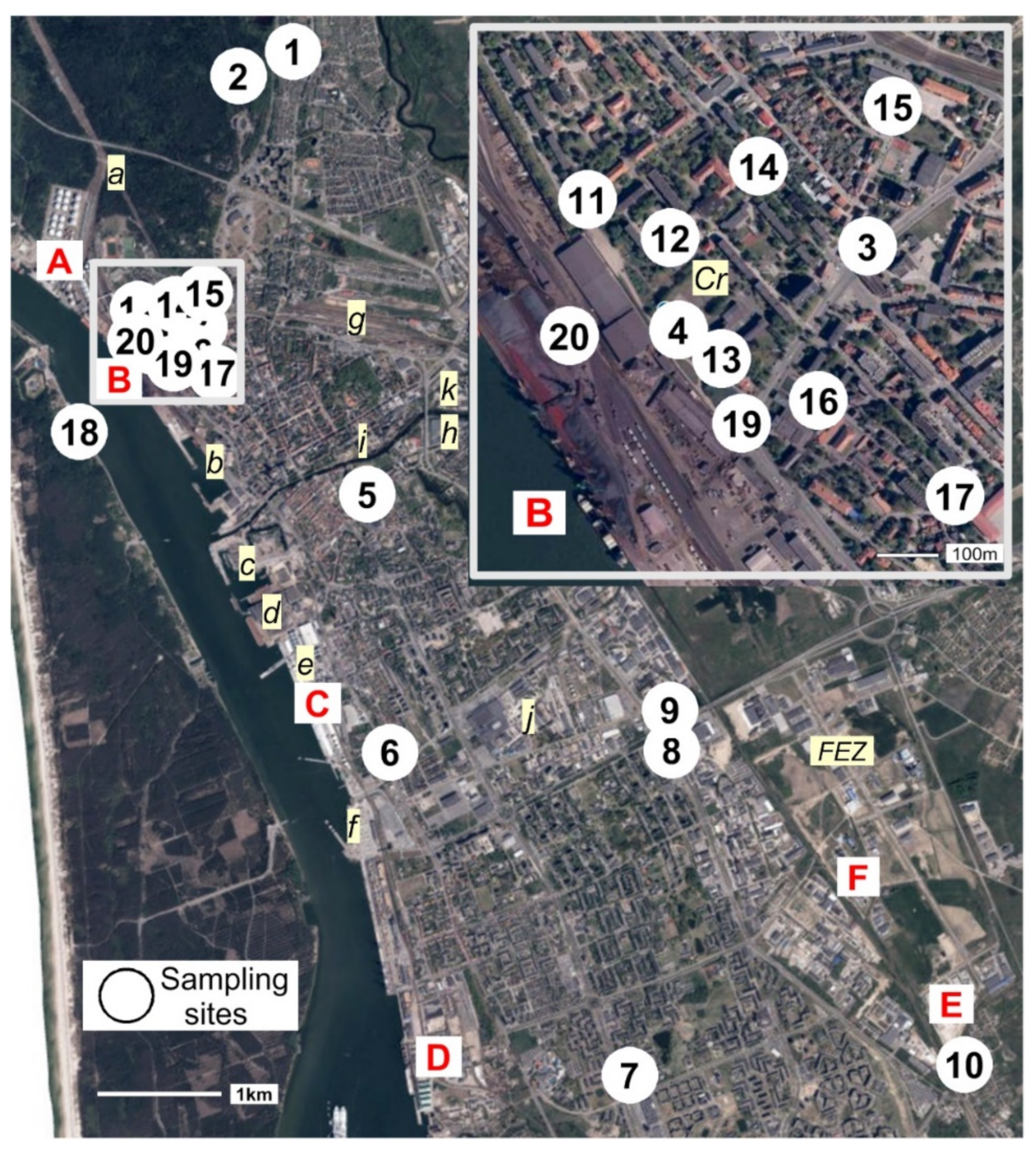
2.1. Study Design

To achieve the main aim of research—i.e., to identify hotspots of contaminants and their emission sources—the following sequence of steps was selected for study design:
(a)
Selection of sampling method of total suspended particles (TSP), samplers, sampling periods, and sampling sites for permanent sampling campaign and extra more dense sampling in sites which are close to iron ore stevedoring (at <1 km distance);
(b)
Sampling of characteristic dust (CD) near the sites of stevedoring particular products. The aim was to obtain information about geochemical composition of products as possible emission sources;
(c)
Analysis of real total contents of selected analytes by EDXRF in accumulated TSP as well as CD, characterizing particular stevedored products;
(d)
Treatment of results by two multivariate statistical methods, i.e., principal component analysis (PCA) and cluster analysis. The tasks were to distinguish specific closely related groups of analytes, to speculate about their possible emission sources basing on findings of other publications, and to compose a list of presumable emission sources for final comparison with real spread of analytes which will be revealed in the last step h via geochemical mapping;
(e)
General ambient air state assessment in Klaipėda with the help geochemical indices (gI) widely used by other researchers in particulate matter (dust) studies. The intention was to find out the possibility of their comparison with respective results of other researchers as well as the usefulness and meaning of their application;
(f)
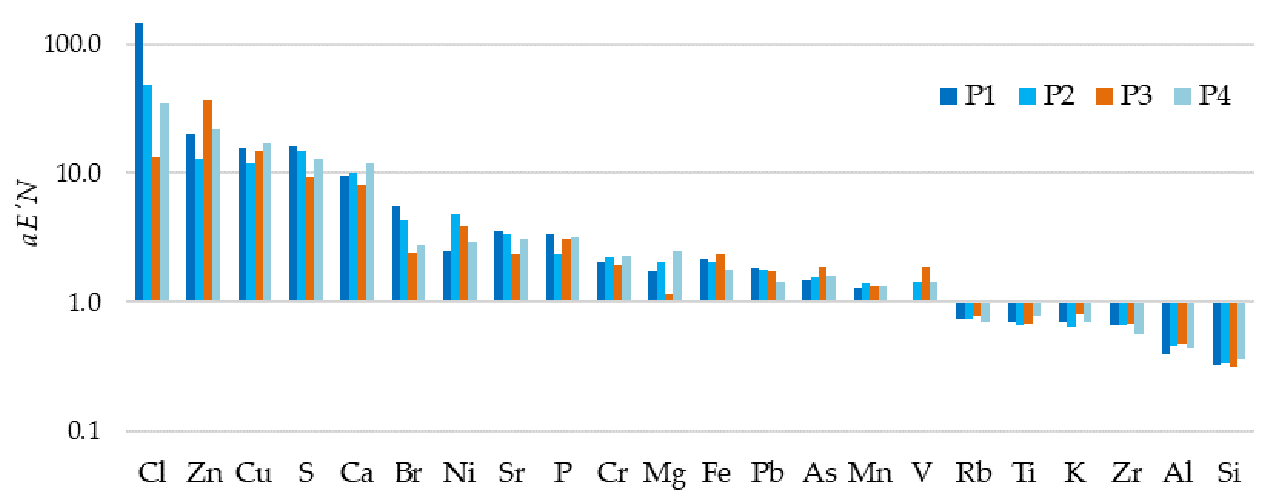
Assessment of temporal variability of the analyte contents during four sampling periods (P1, P2, P3, P4). The purpose was to find out with the help of Friedman ANOVA test the elements which are significantly variable;
(g)
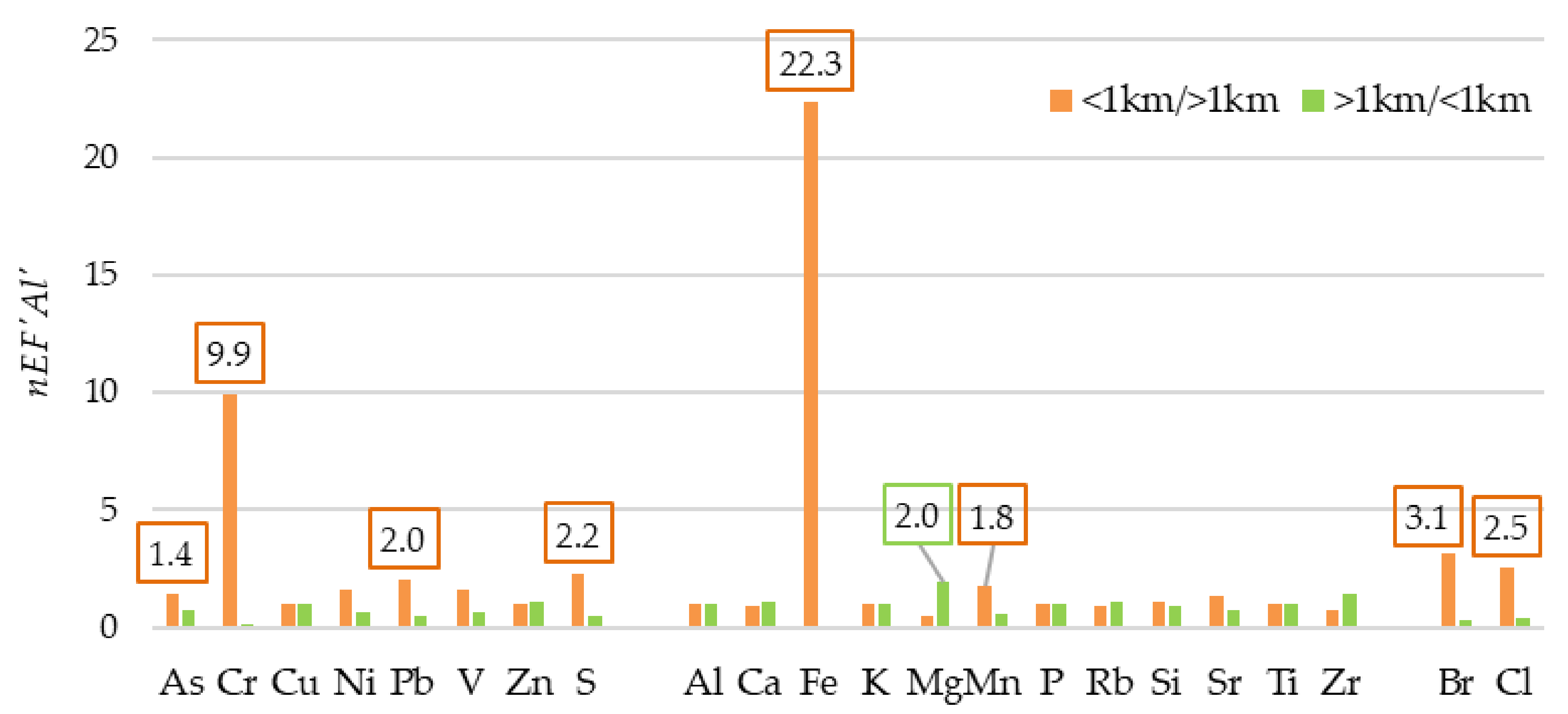
Statistical comparison of gI values in two areas of the city (using nonparametric Mann–Whitney U test): the <1 km area which is close to Fe ore stevedoring and the >1 km area which includes the rest part of the city. The goals were to find out the analytes which have significantly different values in these two areas;
(h)
Mapping of gI values. The purpose was to compare maps with interpretation of multivariate statistical analysis results and data of characteristic dust and to draw conclusions about the reasons of pollutant anomalies.

2.2. Study Area

Klaipėda is an ice-free port city, established in 1252 on the coast of the Curonian Lagoon and the Baltic Sea (55°42′40″ N, 21°7′50″ E). Now it is the third largest city in Lithuania, covers 98 km2, and the population in 2020 was about 150,000. The western industrial zone stretches along the coast of Curonian Lagoon and includes the state seaport with companies involved in stevedoring (having many shipment storehouses), shipbuilding and ship repair; the eastern one includes the “free economic zone” (FEZ) (Figure 1) [21]. The port area covers 540 ha, while FEZ covers 412 ha and has about 100 different companies [22]. Apart from these two large zones, the dense urban structure competes particularly strongly with port and industrial areas. With the growth of the city, some of industrial facilities are already surrounded by residential, commercial, and social zones. An orthophoto map of sampling sites of total suspended particles (TSP) with indicated potential pollution sources is shown in Figure 1.
In Klaipėda, the average annual temperature is +8.5 °C and rainfall is 774 mm; the average monthly temperatures range from −1.4 °C in January to around 19.0 °C in July, while the amount of rainfall is from 41 mm in April to 85 mm in August [23]. The wind parameters during the study periods are presented in Table S1. The study area belongs to Lithuanian Maritime Region with a complicated quaternary geological structure closely related to Baltic Sea development [24]. A simplified scheme of the Quaternary geological map of Klaipėda and discussion on elemental background values levels in topsoil is presented in [25]. According to state departments in 2020 [26], the average concentration of PM10 in Klaipėda was 19.5 µg m−3, while of PM it was 2.5–7.28 µg m−3. However, these values do not address the real state of air quality, especially in the northern part of the city (B locality on the Figure 1).

2.3. Sample Collection

To provide average geochemical composition of urban TSP and its temporal changes, its accumulation was done in the same ten permanent monitoring sites (1–10, Figure 1) by exposing their passive samplers during four sampling periods P1, P2, P3, P4. The exposure of passive samplers during each period in 2020 lasted 6 weeks. The periods were successive: P1—04.03–15.04, P2—16.04–27.05, P3—28.05–08.07, and P4—09.07–19.08. Since sites 1 and 2, 3 and 4, and 8 and 9 are in close proximity, each of these pairs can be treated as one generalized (duplicate) site consisting of two sub-sites; thus, such 7 sites (3 duplicate and 4 single) are evenly distributed in the city. The duplicate sites 3 and 4 are close to iron ore stevedoring. Close to it, an additional 10 sites (11–20, Figure 1) were selected, the location of which around terminal B is denser. In these 10 sites, the accumulation of TSP was done using analogous passive samplers during the same P3 period as in 10 permanent monitoring sites. Therefore, 20 sites were sampled during P3.
Characteristic dust (CD) was collected quite close (“right next door”) at the sites of stevedoring of iron ore, apatite, phosphorite, and potassium fertilizers (analytical data of appropriate samples, named as B’Fe, C’ap, C’ph, and D’KCl will be given in “Results”). Everywhere TSP sampling was done using laboratory-made passive samplers (Figure 2) and only the sample of waste incineration ash (named as F*Wa) was swept from the chimneys.
Samplers were designed with considerations from other research works, with protection from rain and the effects of external factors such as birds or heavy debris. The sampler consisted of a roof (1), a protective net (2), working sections (3), and mounting brackets (4). Disposable Petri dishes were used for sample collection. The area of the single Petri plate was 5674 mm2. Petri dishes were arranged in working sections (3). The Petri dishes were protected from large elements and birds by a net (2). The roof (1) protected the Petri dishes from rain. If water entered the working section, it was collected together with the dust sample using a syringe. The samplers were attached to the electric or light poles at a height of 3 m by means of mounting brackets (4). During the sampling and analysis, extreme caution was ensured in order to avoid contamination of the samples with metallic laboratory tools. Each TSP sample was placed on a microscope slide and a drop of distilled water was added for covering. Photographs were taken using microscope “Nikon Eclipse Ci-L” with a magnification lenses 40×.

2.4. Analysis

Before and after exposition, Petri dishes were dried and weighed. The amount of TSP was determined by the difference in mass. The sampled material was ground to a flour in an agate mortar. From each ground sample, the mixture of 0.5000 g of Licowax binder and 0.1000 g of milled material was prepared, homogenized for 10 min, and a pressed pellet with a 10 mm diameter was made. Each pellet was pressed for ~3 min using 15 KN (Press PP25).
The Wageningen analytical exchange program [27] sample 989 and standards 190 ERM-CZ120, NIST 2702, NIST 2709, NIST 2782, as well DC73022 and DC73317a were prepared pari passu as TSP samples, analyzed, and were used for recalibration. From each of them, three sub-samples were made. The set of all of them was analyzed in triplicate: at the beginning, middle, and end of a series of all studied TSP samples. All pressed pellets were analyzed by energy-dispersive X-ray fluorescence (EDXRF) equipment Spectro Xepos HE (Kleve, Germany) using the TurboQuant (TQ) II for the pressed pellet calibration procedure elaborated by the manufacturers. The TQ method combines different procedures: calculation of the mass attenuation coefficient, using the extended Compton model, and final calibration based on fundamental parameters method. The advantages of polarization and TurboQuant calibration method were described by Schramm and Heckel [28]. The last modification of TQ method, TurboQuant II, intended for Xepos HE, is offered by manufacturers for samples with various matrices [29,30]. Quality control and improving of laboratory results has been performed since 2007 by participation in “International Soil-analytical exchange” (ISE) program organized by Wageningen University [27,31]. From this period, more than 90 ISE reference samples and other certified reference materials were used by current analysis for the recalibration of results.
In this study, Spectro Xepos HE was used to determine the contents of 22 analytes: Mg, Al, Si, P, S, Cl, K, Ca, Fe, Ti, V, Cr, Mn, Ni, Cu, Zn, As, Br, Rb, Sr, Zr, and Pb. For this, each pressed pellet was examined from both sides. The medians of relative standard deviation (%RSD) values of measurements of both sides were <5% for Fe, Sr, Ca, K, V, Rb, Cu, Zn, As, Ni, Zr, Pb, Mn, Br, and S, 5–10% for Cr, P, Ti, Cl, Al, and Si, and 14% for Mg. The minimum determined values of examined analytes in complete dataset of TSP (Table S2) exceeded the lower limits of detection (3 sigma) at least 15,984 for Ca, 4303 times for Fe, 2232 for S, 1154 for Si, 1102 for K, 1093 for Ti, 1030 for Zn, 720 for Mn, 463 for Sr, 247 for P, 133 for Al, 98 for Zr, 94 for Cu, 61 for Br, 42 for Rb, 40 for V, 25 for Cl, 16 for Pb, 5.5 for Cr, 4.7 for As, 2.8 for Ni, and 1.2 times for Mg. The average value of measurements was used for data analysis and statistical treatment, which made it possible to reduce the impact of joint random errors.

2.5. Geochemical Indices

The effectiveness of indices often used by other researchers for general assessment of urban geochemical state and search for potential pollution hotspots and sources will be analyzed. Only indices for calculation of which the natural levels of analytes were taken were examined. The general term “geochemical indices” (gI) was used for them. The indices based on regulatory levels (which are set by legal advices) is not discussed in this study.
To avoid the confusion between indices based on Clarke values (Cv) and those based on native background values (Bn), different letters were used after apostrophe in the abbreviation of each gI: (a) in the first case, the letter was “C” and the source of Cv (for unification) was Rudnick and Gao [32]; (b) in the second case, the letter was “N”.
The following gI was used in this study. The abbreviations in the formulas below are the following: C—the content of selected element in selected site, Cv and Bn are explained above, CAl is the content of Al in site, CvAl is Clarke value of Al, and BnAl is the native background value of Al.
1. Two alternatives of geoaccumulation index Igeo: Igeo’C when Cv is used in the denominator (Equation (1)) and Igeo’N when Bn is in the denominator (Equation (2)).
I g e o = log 2 C / ( 1.5 C v )
I g e o = log 2 C / ( 1.5 B n )
The geoaccumulation index (usual abbreviation Igeo) was introduced by Muller for classification of river sediments according to contamination level [33]. Presently Igeo is widely used by researchers for classification of contamination not only of sediments or soil, but also of dust, e.g., [34,35,36,37] and others. They apply the same rule to distinguish dust contamination level, i.e., seven Igeo-classes earlier used for evaluation of river sediment contamination [38]: 0 (Igeo < 0)—uncontaminated, 1 (Igeo: 0–1)—uncontaminated/moderately contaminated, 2 (Igeo: 1–2)—moderately contaminated, 3 (Igeo: 2–3)—moderately/strongly contaminated, 4 (Igeo: 3–4)—strongly contaminated, 5 (Igeo: 4–5)—strongly/extremely contaminated, 6 (Igeo > 5)—extremely contaminated.
2. Two variants of normalized enrichment factor nEF based on Al as reference element: nEF’Al’C when Cv is used in the denominator (Equation (3)) and nEF’Al’N when Bn is in the denominator (Equation (4)).
n E F A l C = ( C / C A l ) / ( C v / C v A l )
n E F A l N = ( C / C A l ) / ( B n / B n A l )
The term “normalized enrichment factor” (with abbreviation Fxn) was firstly proposed by Rahn [39]. Presently normalized enrichment factor is widely used and usually entitled “enrichment factor” without the word “normalized” and with abbreviation EF. It was used for dust studies by some researchers, e.g., [36,40,41,42] and others. Now this index is sometimes used for dust contamination classification, e.g., [43,44,45], to distinguish five so-called contamination classes (SCC): <2—minimal; 2–5—moderate; 5–20—significant; 20–40—very high; >40—extreme.
However, more often the researchers use nEF index to distinguish the presumable origin of analytes in dust, i.e., natural or anthropogenic. Most commonly the researchers citing previous publications accepted nEF < 1 to indicate significant terrigenous (crustal) origin, while nEF > 10—significant anthropogenic contributions [45,46,47].
3. Index of potential atmogenic enrichment of topsoil aE’N (Equation (5)).
a E N = C / B n
The analogous ratio of aerosol concentration to soil concentration was firstly used in 1971 by Rahn and was entitled as “enrichment factor” (abbreviation Fx) [39]. But since many researchers now use the term “enrichment factor” (abbreviation EF) for another index which was entitled by Rahn “normalized enrichment factor” (abbreviation Fxn) [39], to avoid confusion, we use another title and another abbreviation (instead of previous Fx) in our study: aE’N. The letter “a” means “atmogenic”, the letter “E” means “elemental enrichment” and the term “factor” is changed to “index”. In soil or dust studies, the index aE’N is also sometimes entitled as “elemental concentration coefficient” (KC or KK) [14,48,49,50]. The identical formula (Equation (5)) is used in dust studies to calculate contamination factor CF [51] with the reference to Hakanson as primary source [52]. Although Hakanson used the index for lake sediment classification into four levels of CF, the same classes are used for assessment of dust contamination level [51]: <1—low; 1–3—moderate; 3–6—considerable; >6—very high. First of all, we would like to turn attention to the identity of sites classed based on non-logarithmic aE’N data to SCC with the integers 3 and 6 as thresholds (THR) and classed according to logarithmic Igeo data to SCC with THR values 1 and 2. But there is lack of such correspondence between classification of logarithmic and non-logarithmic data for higher SCC. If the higher THR values for classification of Igeo’N (3, 4 and 5) are back-transformed to integers to be used for classification of non-logarithmic aE’N data, the respective four intervals will be 6–12, 12–24, 24–48 and >48. This classification is more detailed in comparison with that used for aE’N by [51] where the aforementioned four intervals belong to solely one interval >6. The uppermost THR used by [51] for classification of aE’N reduces the sensitivity of this index for recognition of hotspots formed by some analytes. From this point of view, the index Igeo‘N is more useful.
The choice of either Cv or Bn can lead to different general formal conclusion about ambient air state. The resulting uncertainty, when the same name is used for indices based on either Cv or Bn is being addressed by a growing number of researchers such as [36,40,41,42] and others. Therefore, we shall try to compare data classifications according to SCC in discussion, where the effectiveness of search for presumable contamination hotspots and sources will be analyzed.

2.6. Data Treatment and Statistical Analysis

The Bn values used in this study were determined earlier [21] using topsoil analysis data set from the same Klaipėda territory where dust was sampled for this study. Microsoft Excel was used to calculate the main statistical parameters of elemental contents in dust and the values of aforementioned gI, while STATISTICA 9 software to perform other algorithms. They were the following: (1) hierarchical cluster analysis by Ward’s method using 1-rP distance where rP is Pearson’s correlation coefficient; (2) principal component analysis (with varimax normalized rotation); (3) testing of different non-parametric hypotheses by Mann-Whitney U-test and Friedman ANOVA test. U-test helped to reveal significant differences in elemental contents and gI between two areas, while Friedman ANOVA test to study temporal variability of chemical elements during four study periods.
Multiple classed post maps for Igeo’C, Igeo’N, nEF’Al’C and nEF’Al’N indices were prepared using the Surfer Golden Software. Each figure presenting maps consists of three panels (a, b, c), in the first two, the values of each gI index are classified into levels corresponding to so-called contamination classes (SCC), while in the last one (panel c) according to presumable origin. In order to adapt nEF’Al’C and nEF’Al’N indices to the discussion about dominant contribution (crustal or anthropogenic) of each analyte, the main thresholds 1 and 10 in panel c were used.

3. Results

3.1. Reasons of Artificial Passive Samplers Selection

Artificial passive samplers’ choice was a result of attentive review of literature about PM sampling methods. Due to the main advantage of continuous accumulation of sufficient dust for quantitative analysis, it was decided to use artificial passive samplers for the study. Although wide range of PM sampling methods is available worldwide, including biotic accumulators, e.g., lichens, moss, barks, leaves [1,14,53,54,55], and abiotic passive methods, i.e., (i) sampling of dust deposited on snow cover [15,48,56,57,58], (ii) sampling of road dust from pavement using a brush and a scoop [42,43,59,60,61,62,63,64,65], the main advantages of artificial passive samplers are: they are cost friendly, have a known deposition period, measurement of deposition flux, and have the possibility to provide important indicators for local pollution sources [2,65,66,67,68,69,70,71].

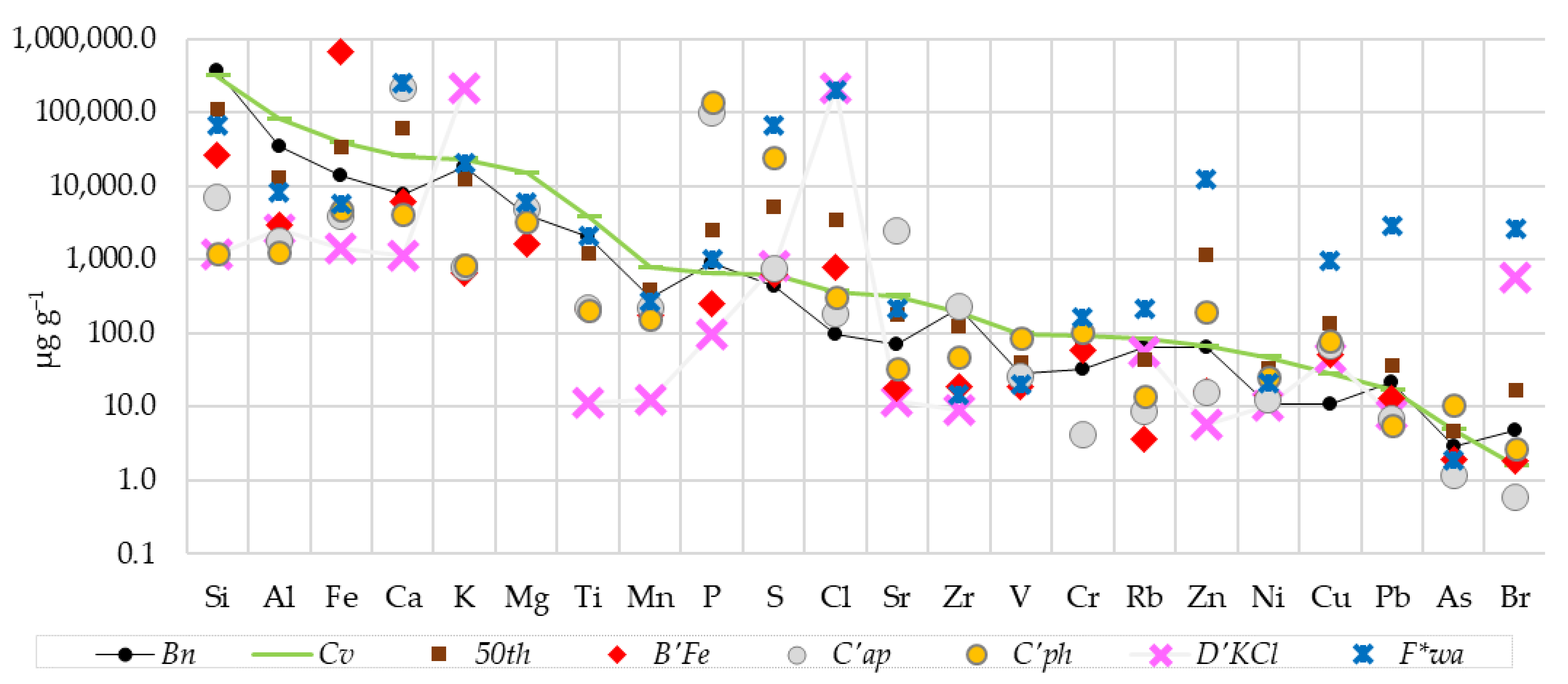
3.2. Main Geochemical Characteristics of Dust

Chemical elements and selected statistical characteristics of their contents in dust (Table S2 and Figure 3) are arranged according to descending Clarke values (Cv), i.e., mean contents for the upper continental crust which were entitled by the name of the first researcher [72] who published such data. Clarke values were taken from data listed in [32]. They represent composition derived from eleven publications, firstly given in [72]. Examination of the native topsoil background values Bn of the study area shows that native topsoil of Klaipėda has only five analytes with mean values exceeding Cv by more than 13%, i.e., Si, P, Zr, Pb, and Br, while the contents of other 17 analyzed elements are lower: Zn by 6.3%, Al, Fe, Ca, K, Mg, Mn, S, Cl, Sr, V, Cr, Rb, Ni, Cu, and As by at least 27%.
It should be noted that median content of Fe (29.6%) in the living area dust sampled near stevedoring of iron ore (<1 km) was only 2 times lower than respective content in the characteristic dust of stevedored iron ore (BFe is 65%). Only Soltani et al. [73] reported a 20% Fe content in the outdoor TSP in the environment of Gol-E-Gohar mining and industrial complex.
Comparison of elemental contents in emitted dust of each stevedored production itself with Bn shows that the elements can be arranged in the following sequences of descending aE’N values (we take into account enrichment not lower than 1.3 times): (i) iron ore dust (BFe)—Fe(aE’N = 48) > Cl (7.8) > Cu (4.7) > Cr (1.8) > S (1.5) > Ni (1.3), (ii) apatite dust (Cap)—P (109) > Sr (34) > Ca (27) > Cu (6.4) > Cl (1.9) > S (1.7), (iii) phosphorite dust (Cph)—P (152) > S (56) > Cu (7.4) > As (3.7) > Cl (3.2) > Zn, Cr, V (3.1) > Ni (2.3), (iv) potassium fertilizers dust (D’KCl)—Cl (2118) > Br (119) > K (12) > Cu (4.4) > S (1.9). It should also be noted that waste incineration ash (F*wa) had Cl content exceeding the Bn level 2049 times, Br—556 times, Zn—201, S—150, Pb—136, Cu—92, Ca—31, Cr—5.0, Rb—3.3, Sr—3.0, Ni—1.9, and Mg—1.5. It means that in case of uncontrolled spread into environment of part of such ash, it will become additional component of contamination. The formal permit given to the waste incineration plant (site F in Figure 1) for emissions of pollutants into ambient air) confirms the possibility that this company can be one of emission sources of Cl, S, and PM with various chemical compositions. But it should be noted that the release of Br has not yet been requested in formal permit, although some studies, e.g., [74], confirm this possibility.

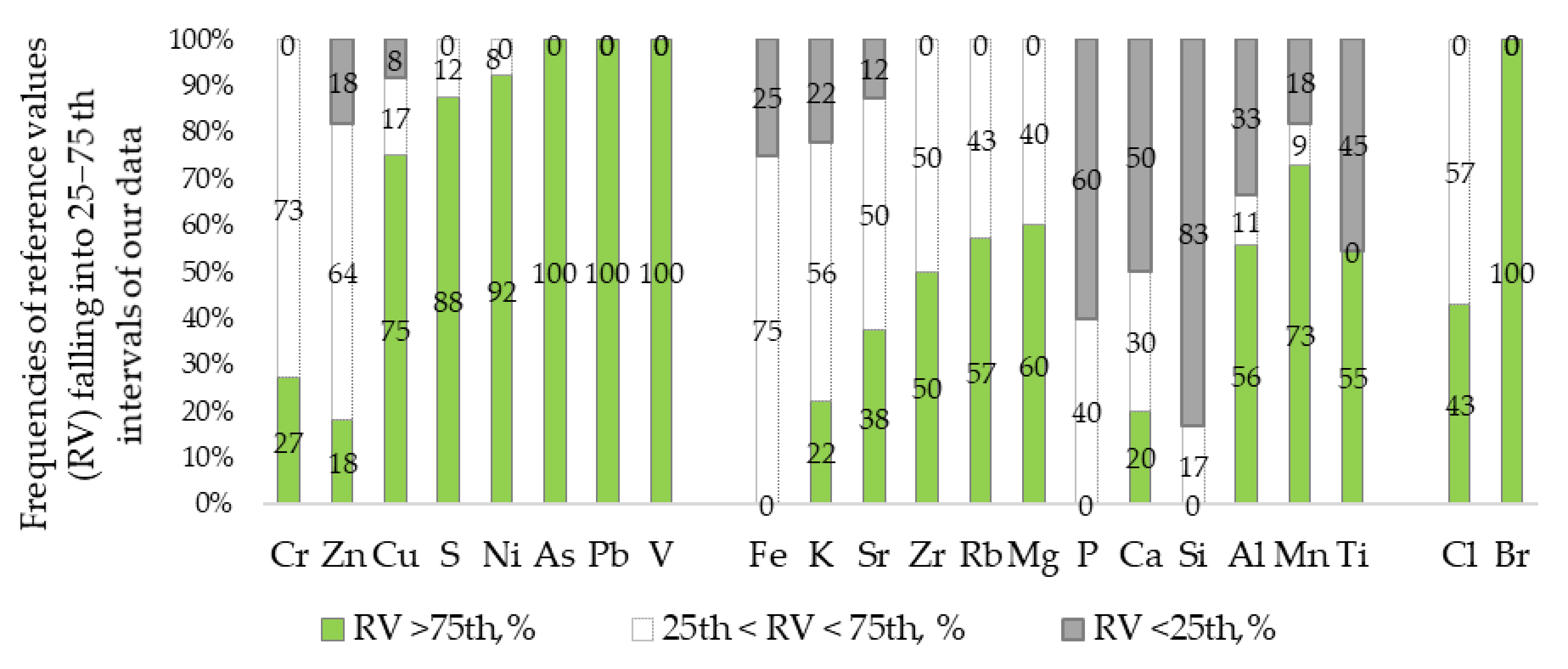
3.3. Our Elemental Contents and the Published Data

To minimize possible temporal differences, we searched only for publications where dust was sampled not more than 15–20 years ago. The next criteria in search of information for comparison with our elemental contents were to avoid data determined by quite different analytical methods and to choose studies with results of the real total contents of elements [31]. If measurements were done not by XRF or INAA (without digestion), but by ICP-ES, ICP-MS or AAS, only the studies where HF (with other acids) was used to digest the samples were selected (Table S3). The third criterion was dust particle size. As we have shown (Figure 4), only in exceptionally rare cases did the dust particles sampled in Klaipėda fall into the interval 50–100 μm or exceed it.
Therefore, the data of studies where road dust researchers consider <250 μm fraction [60] or even larger particles, e.g., <500, <1000, or <2000 μm [75,76], as dust were not chosen for comparison. Moreover, we refused with great regret from publications with some other strange data: (i) where the given mean contents of several analytes, for example, Ti and Cr in mg kg−1 are only 0.024–0.02 and 0.023–0.02 [77], since they are below the detection limits of XRF; (ii) where the sum of the contents of studied chemical elements is 100% and in one case is even 128% [78]. We also could not access the required data from some publications, e.g., [79], because only the volume concentrations (ng m−3) of analytes were presented without indicating the concentration of dust (μg m−3), therefore their re-calculation to mass concentrations was impossible.
According to the aforementioned selection criteria, some publications such as [66,80,81] seemed to be appropriate information sources for comparison with our TSP data (Table S3). We also present for comparison the elemental results of dust: (i) collected from the snow cover [56,57], (ii) caught by pumping PM10 and PM2.5 from air above the ground [18,82,83,84], (iii) “inhalable road dust particles sucked directly” from the pavement [8,35].
A review of the selected publications revealed that the differences in elemental contents may be determined not only by objective factors such as anthropogenic or natural specificity of research area, but also by subjective features of sampling, sample preparation and conditions of analysis. Sampling alone depends on (Table S3): (i) sampling time, e.g., year, season, prevailing momentary meteorological conditions; (ii) specific location of sampling site and certain height above the ground (for unknown reasons, the height is even not indicated in some studies); (iii) sampled particle size and sampling tools. Therefore, the comparison of such data has uncertainty. With this in mind, for each element, the correspondence (%) between our and selected published data was estimated by percentage of reference values within the 25th–75th percentile interval of our study (Figure 5). The arrangement of PHEs according to descending correspondence is Cr > Zn > Cu > S > Ni. It should be noted that the mean values of PHEs As, Pb, V, as well as of halogen Br given by other researchers exceeded our 75th percentile. The crustal elements were arranged as follows: Fe > K > Sr, Zr > Rb> Mg, P > Ca > Si > Al > Mn. Halogen Cl (57% correspondence) appeared among the analytes (Fe > Cr > Zn > K) with higher than 50% correspondence.
It was found that when choosing the analytes, researchers give priority to PHEs. Nevertheless, the group of elements with most frequent (75–100%) choice for analysis included not only PHEs Ni, Pb, Cu, V, Cr, Zn, but also some crustal elements, i.e., Fe, Mn, Ti, and Ca (Figure 6). The frequency of selection PHEs As and S, crustal elements Al, K, Sr, Rb, and halogen Cl was 50–75%, of Si, Mg, P, and Zr was 25–50%, while of halogen Br was below 25%, i.e., it is analyzed most rarely.

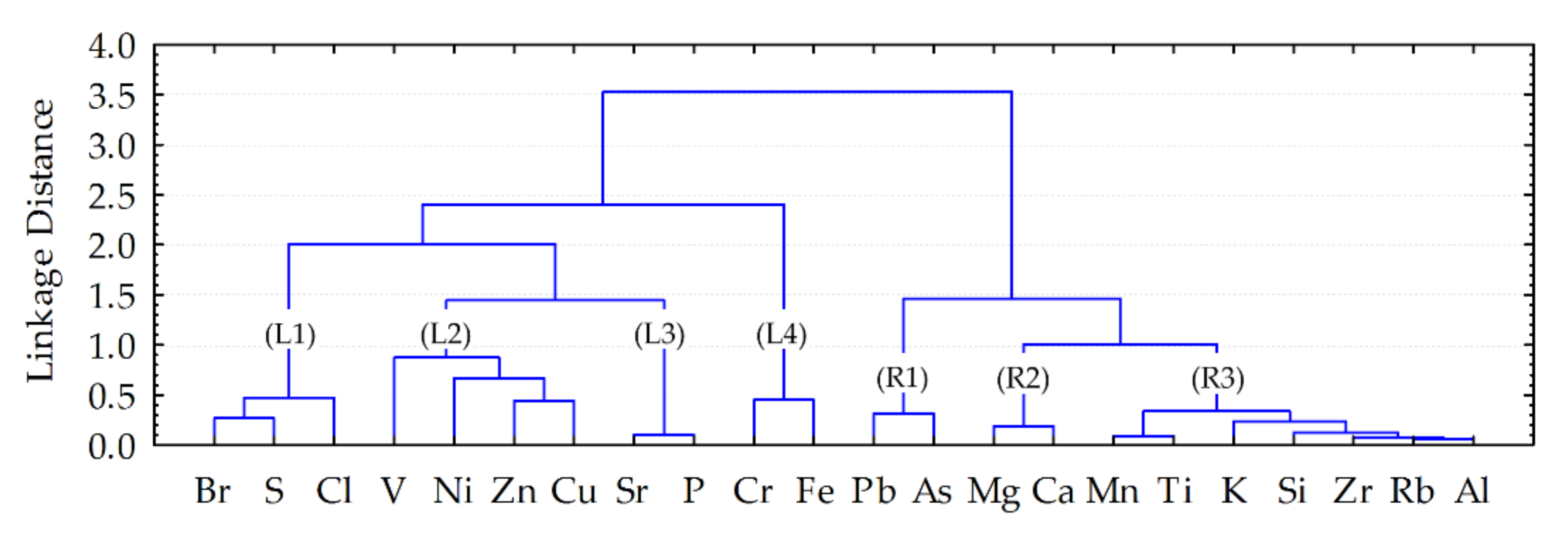
3.4. Factor Analysis and Clustering of Complete Datasets

Five factors explain 79% of total geochemical variance of complete dataset TSP (Table S4) and their loadings significant at p < 0.01 are listed in parentheses: F1TSP (Rb, Al, Si, Zr, K, Mg, Mn, Ti, Ca, Cu, –Cr, –Fe), F2TSP (P, Sr, Ca), F3TSP (Br, S, Cl), F4TSP (Zn, V, Cu, Ti, –Mg), F5TSP (Pb, As, Cr, Mn). Cluster analysis of such dataset demonstrates two main branches of dendrogram joining together at a linkage distance (LD) 3.5 (Figure 7). The left branch consists of four clusters, i.e., (Br–S)–Cl (L1), V–(Ni–(Zn–Cu)) (L2), Sr–P (L3), and Cr–Fe (L4). The right branch is composed of three clusters, i.e., Pb–As (R1), Mg–Ca (R2), and (Mn–Ti)–(K–(Si–(Zr–(Rb–Al)))) (R3). The same nine elements Rb, Al, Si, Zr, K, Mg, Mn, Ti, and Ca which are in clusters R2 and R3 have the highest positive loadings (>0.69) on F1TSP factor. Part of R3 elements, i.e., Al, Rb, Zr, Si, K, show very close association (LD < 0.25) and have the highest (>0.85) loadings on F1TSP (Table S4).
Quite different relationship was revealed in topsoil background sites of Klaipėda (Table S4): Nine elements which determine the variance of factor F1TSP were distributed in the loadings of three factors of background topsoil: F1BT, F2BT, and F3BT. Factor F1BT showed marked antagonism between Si (indicator of sandy soils) and tracers of clayey soils in unpolluted (background) areas Al, Mg, Ti, and Fe. A similar separation of Si from elements clayey component indicators was characteristic of European topsoils and was visible from cluster analysis dendrograms [85]. The variance of factor F2BT was determined by other three of aforementioned nine elements, i.e., Zr, Rb, and K, while of F3BT by remaining Ca and partly (at p < 0.05) also Mg. In background topsoil, factor F1BT was loaded not only by Al, Mg, Ti, Fe, and Cu, but also by Ni, V, and Cr. However, in dust factor F1TSP, Cr as well as Fe were obvious antagonists of Al, Mg, and Ti, while V, Ni and Cu as well as Zn and Ti had positive loadings on F4TSP and were antagonists to Mg.

4. Discussion

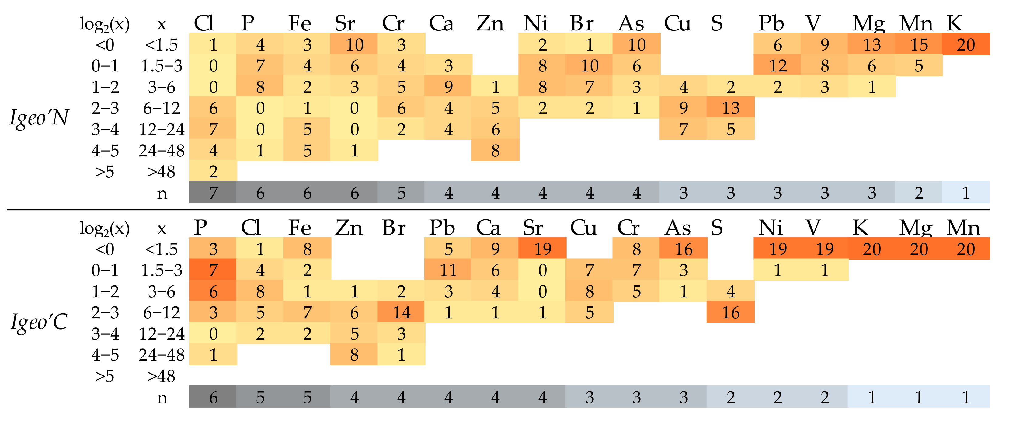
4.1. Geochemical Indices and So-Called Contamination Classes

The mean values of geochemical indices used in this study (gI), i.e., Igeo’C, Igeo’N, nEF’Al’C, nEF’Al’N, and aE’N (Table S5), in seven evenly distributed sampling sites during four periods from 04.03.2020 to 19.08.2020 are discussed, aiming to compare them with respective values from published data. In each from three paired sampling sites 1 and 2, 3 and 4 and 8 and 9 which are close to each other (Figure 1), the results are averaged for each period to obtain more even distribution of gI values in the study territory. The uncertainty of contamination level estimated by Igeo resulting from different Cv or Bn values in the denominator of formula, was demonstrated by e.g., Dytłow and Górka–Kostrubiec [36] and other researchers. It is also obvious for Klaipėda, from comparison of so-called contamination classes (SCC) distinguished according to two alternative Igeo indices. If the mean Igeo’C was selected instead of the mean Igeo’N, the estimated SCC of nine analytes, i.e., Cl, Cu, Ca, As, Fe, Sr, Ni, Cr, V (with asterisks in Figure 8), would be lower, while by Br would be higher. Hence, the choice of Igeo’C would lead to conclusion about cleaner ambient air in Klaipėda. The answer to the question why most analytes in TSP of Klaipėda have higher Igeo’N values in comparison with Igeo’C and there are only five of them (Br, P, Pb, Si and Zr) which have lower Igeo’N values is in the ratio of Cv and Bn: the higher this ratio (Cv/Bn in Table S5), the higher the difference.
When using alternative normalized enrichment factors nEF, the differences in assignment to SCC are also seen. In comparison with nEF’Al’C, the mean nEF’Al’N values of Br, S, P, Pb, K, Zr, Rb, Si, and Ti distinguish lower SCC and the city dust was entitled as less contaminated by them, while the mean nEF’Al’N values of Ca, V, and Sr resulted in higher SCC (Figure 9). Similarly, to Igeo, these differences were determined by Cv and Bn values, but in this case, of two elements: (i) for which the index was calculated; (ii) the reference element used for normalization. In our case, the latter was Al (Formula (4)), therefore for the selected element, the ratio of alternative nEF values nEF’Al’C/nEF’Al’N was a constant value, calculated as follows: (CvAl/BnAl)/(Cv/Bn) (Table S5).
Since the number of possible different SCC for two aforementioned indices is not equal (seven for Igeo and four for nEF), we compared the frequency of attribution of analytes to the SCC which are higher than “moderately contaminated” (Section 2.5), i.e., the number of so-called more strongly contaminating analytes (CA). When using Igeo‘C (when Cv is in the denominator) CA = 4, i.e., Zn > Br > Cl > S, while in case of nEF‘Al‘C, CA = 12, i.e., Zn > Br > Fe > S > Cl > P > Cu > Cr, Pb > Ca > As > Ni. For Igeo‘N (when Bn is in the denominator), CA = 5, i.e., Cl > Zn > Cu > S > Ca, for nEF‘Al‘N, CA = 13 (Fe > Cl > Zn > S > Cu > Cr > Ca > P, Br > Ni > Sr > As > V). Thus, whichever alternative of Igeo index (either Igeo‘C or Igeo‘N) was used for assignment to a specific SCC, the general ambient air state in Klaipėda according to SCC title would seem better than using each of alternative nEF’Al indices.
However, the greatest confusion is caused by generalization of results when the study territories were compared only according to the SCC title. For example, according to As, both dust of Klaipėda (Table S5: mean As is 5.26 µg g−1, so IgeoN = 0.04) and dust of Guilin (IgeoN = 0.13) [86] were attributed to the same SCCuncontaminated to moderately contaminated”. However, soil related Bn value of As used for calculation of this index in Guilin was 20.5 µg g−1, while Bn used in Klaipėda was 2.9 µg g−1. Taking into account the formula (2), we found that the mean value of As in dust of Guilin was 33.6 µg g−1. Let us suppose that such an As content was determined in Klaipėda dust. In this case (Table S2: Bn is 2.9 µg g−1), the SCC for As in Klaipėda became “moderately/strongly contaminated” (Igeo would be 2.95), i.e., formally, dust would be considered as much more contaminated than in Guilin. But does this mean that the residents of Guilin inhale much cleaner ambient air than in Klaipėda, when the detected real content of As in dust of Guilin (33.6 µg g−1) is even 6.4 higher than in Klaipėda (5.26 µg g−1)?
Maybe due to various aforementioned reasons, there are a lack of manuscripts where the researchers provide responsible comparison of SCC distinguished by them using gI of dust with data presented in other publications. After attempts to compare their results with data published by others, Zglobicki et al. [44] politely but aptly notice: “This shows the difficulty of directly comparing results obtained for various cities. The main challenge here is the method of determining the geochemical background that plays a key role in the case of some pollution indices”.
Taking into account the material of this subsection we dared to propose to refuse from using the term “contamination classes”, if they are distinguished according to geochemical indices of dust. Classification into such classes was firstly applied not for dust (Section 2.5). The attempts to adapt gI for dust without changes of terminology often cause confusion, since the assignment to certain SCC is understood in the society as the index of ambient air contamination. However, this assignment is related to subjective factor, i.e., when different values are taken in the denominator (Equations (1)–(4)) during calculation of gI, so manipulations are possible. Even small difference in selected Cv values (the study of Rudnick and Gao [32] contains data of all eleven compilers of Clarke values) or Bn values the problems of selection of which have been described by us [25,87], can determine attribution of sample to different SCC. However, whichever unique Cv or Bn value is chosen, the level of analyte content in ambient air is the same. In general, we do not object to using some of geochemical indices, like Igeo or aE (Kk), for evaluation of dust relative contamination level using the terminology “less”, “more”, or “most” contaminated only within the dataset which is studied. However, the terminology should be selected responsibly and purposefully as much as possible. Having in mind that either soil- or upper continental crust-related values are in denominators of Igeo’ formulas, when using them, the term “enrichment” can be proposed instead of the terms “contamination” or “pollution”. Following Rahn [39], we tried to apply namely such terms (“enrichment”) for aE‘N (Section 2.5). For example, in the case of Igeo‘N, the term “(top)soil-enrichment Igeo index”, while in case of Igeo’C—“Clarke enrichment Igeo index”, or similar alternatives can be used.
In our opinion, normalized enrichment factors cannot be used for naming “contamination classes”. Their purpose is different: help in attempts to find out the origin of presumable contaminant in dust, probably also the emission source of dust and hotspots formed by it. Namely for this aim they are most commonly used, although there is warning about their indiscriminate usage [88,89]. As was noted by Cesari [40], when using normalized enrichment factors, it is especially important to provide the following information: (i) the reference element selected; (ii) publication from which the reference values are taken.

4.2. Weather Changes as a Factor of Dust Elemental Contamination Variability

The magnitudes of median aE’N demonstrate that Cl, Zn, Cu, S, Ca, Br, Ni, Sr, P, Cr, Fe, Mg, Pb, As, V, and Mn have the dominant potential to create their own atmogenic pedogeochemical anomalies in any of the study periods P1, P2, P3, and P4 (Figure 10).
Moreover, variability of Cl, S, Sr, Ni, Br, V, and Zn is significant at p < 0.05 (Table S6). Four of these seven analytes, namely Cl, Br, S, and Sr, have a similar pattern: period P3 is characterized by their lowest median aE’N values compared to other periods P1, P2, and P4. The prevailing wind directions during P1, P2, and P4 were from the sea, since the sums of the frequencies of W, NW, and SW directions were 53%, 61%, and 57%, while during P3, the sum was only 27% and two opposite directions, i.e., NE and E, comprised 49% (Figure 11).
It is possible that higher wet precipitation during P3 (Table S1) brought from the continent diluted the sea sprays and washed out the atmosphere decreasing the content of dust. Such phenomenon has been demonstrated in [90]. It was found that when the winds were blowing from the sea (SW–W–NW sectors), the averages of median aE’N values of all three periods P1, P2, and P4 for Cl, Br, S, and Sr were 17.4, 5.2, 4.7, and 4.2 times higher than the respective contents during P3. The common possible origin of three analytes (Cl, Br, and S) was confirmed by their strong positive loading on factor F2TSP (Table S4) and amalgamation in cluster L1 (Figure 7). Strontium belongs to cluster L3 (Sr–P) which is adjacent to L1. Thus, it seems to us that in the case of Klaipėda, the presence of S together with obvious marine origin indicator Cl and Br [91] should not be surprising: Cl and Br, accompanied by S, are among the main indicators of waste incineration ash and potassium fertilizers stevedoring, while Cl and S are indicators of phosphorite and apatite (Table S2 and Figure 3). The variability of Sr contents can be related with these analytes due to apatite (source of Sr, Cl, and S) and phosphorite (S, Cl) stevedoring simultaneously with potassium fertilizer (Cl, Br, S) operations. Contrary to Cl, Br, S, and Sr, the patterns of Zn and V median aE’N values were similar in reaching maximum in P3 period, while the peak of Ni was in P2. During P3 with prevailing offshore winds, Ni, V, and Zn had 2.7, 2.1, and 1.5 times higher median aE’N values than respective averaged values of median P1, P2, P4 levels. Davulienė et al. [12] state that the western air masses were mainly associated with moderately polluted air flow from Western Europe, particularly from the UK, Denmark and North Poland.

4.3. Inter-Elemental Relationship and Related Groups

In a Belgium study, Al, Si, Ti, Ca, K, Mn, and Fe which have loadings >0.5 on the first factor (see Table 4 in [82]) are interpreted as crustal. In Krakow, the origin of Al, Si, K, Mg, Ca, and Fe which are clustered separately (see Figure 7 in [92]) is interpreted as natural. Separation of a few aforementioned elements can also be found in other publications: e.g., Al, Fe, K, Mg [81], Al, Fe, and Mn [93]. Most of these elements are considered as crustal in review of various studies, too [94]. Iron was always among them, provided it was determined. But in the case of Klaipėda, Fe does not associate with all these crustal elements, and it is distinguished as their strict antagonist (see F1TSP in Table S4). Cluster analysis confirms this, since cluster L4 composed of Fe accompanied by Cr is in the left branch of the dendrogram and is separated from other crustal elements in the right branch (Figure 7). Such separation of Fe from other crustal elements enables us to presume that it has its own emission source. The antagonism between Fe and crustal elements which is expressed in factor F1TSP indicates that significant Fe input notably reduces the re-suspended part of other “traditional” crustal elements. This powerful source of Fe has clearly other origin than diffuse anthropogenic sources of Fe and associated with them elements which in Belgium were interpreted as “traffic and metals” (see the fourth factor in Table 4 [82]). In the dust of Klaipėda, similar Fe sources also exist, but are reflected in another factor, F5TSP, as can be seen from significant at p < 0.05 loadings of Pb, As, Cr, Mn, Fe, and Ni on it. Almost all analytes in this list are also in aforementioned fourth factor, except Ni.
Still, we cannot deny native source of Fe mentioned in all previously cited publications [81,82,92,93] where positive correlation of Fe with other crustal elements has been shown. We can presume partial pedogenic origin of Fe in dust of Klaipėda basing on: (i) conclusions of these researchers, (ii) the fact that L4 cluster in the left branch of the dendrogram is the closest to the right branch and only two connections separate it from clusters R2 and R3 which include crustal elements, (iii) undeniable association of Fe with other crustal elements which is observed in topsoil (see Fe loadings on FTBT and dendrograms in our previous research of topsoil background composition [25,87]) which serves as a source of re-suspension. But presently, Fe ore stevedoring seems to be not essential source of Cr, since the highest loading of Cr is on F5TSP, i.e., it belongs to the group of elements leaded by Pb and As and accompanied by Cr, Mn, Fe, and Ni. Extremely high contents of Cr together with Fe have been observed in topsoil of the northern part of the city near Fe ore stevedoring terminal since 2005 [21,95] up to today [96]. This part of the city has the oldest history and has been influenced by anthropogenic activity for the longest time. Lead was earlier an important traffic-related element because of leaded gasoline [97,98]. The anomalies of Pb are the most conservative compared to other PHEs, i.e., best of all repeat their primary configuration, although the level of Pb in them inevitably decreases [14]. Relatively close to oldest part of the city (site i in Figure 1), one of the greatest factories of galvanic batteries in the former USSR has been operating since 1989, and it polluted the surrounding topsoil with Zn, Cu, As, Ni, Pb, Mn, Sr, and Cr [21]. Therefore, according to our available data, resuspension of formerly contaminated topsoil can be the most probable reason of elemental grouping in F5TSP and R1.
The next factor F2TSP according to percentage of explained variance (12%) is significantly (p < 0.01) loaded by Sr–P–Ca. Two of these three elements, i.e., P and Sr, form their own cluster L3 in the left branch at the lowest distance LD < 0.2. It is known that association Sr–P–Ca is characteristic of apatite-group minerals [99] and phosphorus fertilizers produced from them. High content of Sr can be found in superphosphate, although it depends on raw material: igneous rock phosphates contain more Sr than sedimentary [100]. This difference is also confirmed by our data (Table S2). Having in mind that the chemical industry company “Lifosa” operates in Kėdainiai (Lithuania) is one of the greatest phosphorus fertilizer manufacturers in Europe [101], the production and raw materials of which are stevedored in Klaipėda, successful fixation of its emissions with the help of factor and cluster analysis is quite accurate.
Side-by-side to Sr–P linked up in L3 cluster, there the is ((Cu–Zn)–Ni)–V group which constitutes L2 cluster. Further, amalgamation of both clusters takes place in earlier stage than with other clusters in the left branch of the dendrogram. Factor F4TSP corresponds to L2 cluster. In comparison with Bn, the increased contents of Cu, Zn, Ni, and V are found in the dust of stevedored phosphorites. However, Zn and Cu are distinct indicators of various anthropogenic activity, first of all, urban traffic. Brake wear and exhaust emissions (fuel, lubricating oil, and motor wear) have been shown as responsible for emissions of Cu, Zn, and Pb [102]. Cluster of Zn and Cu with Pb and oil products in the topsoil of the central urban districts of Vilnius also confirms this [48]. Presumably, shipbuilding and ship repair [103] is also one of Zn and Cu sources. Both elements are tracers of waste incineration plants, too [104], and geochemical composition of ash from Klaipėda waste incineration plant does not deny this finding (Table S2). Another two indicators of anthropogenic activity, i.e., Ni and V, are close to pair Zn and Cu. Heavy oil used in boilers [15,94], as well as used in marine engines [18,105,106] has high contents of these elements. These facts enable to presume that part of V and Ni can be transferred to ambient air due to shipping activity. Besides, one should have in mind that the impact of “Mažeikiai Refinery” [107] which is one of the greatest oil refineries in the region and is located only at 110 km northwest from Klaipėda is also possible.
In the next stage, cluster L1 composed of anionic elements Br, S, and Cl link up with joint cluster L3 + L2. The same three elements have significant loadings on respective factor F3TSP. There is usually little doubt that Cl originates from sea salts [82,84,108], meanwhile statements about marine origin of Br [109] and S [110] are rather rare. The latter circumstance can be predetermined by lack of Br measurement data (Figure 6). For example, in the Belgium study [82], Br content was not presented, although the equipment used allowed its reliable determination. Chlorine, S, and Br are sensitive to meteorological conditions (Table S6). This affinity can determine the possibility that some their proportion appears in Klaipėda by long-range atmospheric transfer, dominant from western directions of Europe [12]. The data of S and Br in Table S3 does not deny this. The concentration of S in PM10 of Belgium (value of for “all stations” given Vercauteren et al. in [82] is 2080 ng m−3, after recalculation to mass concentration in dust it is ~70,034 µg g−1) more than 13 times exceeds the median value in TSP of Klaipėda. The explanation of such a difference solely by the capability of finer particles to accumulate pollutants is insufficient, because e.g., Wang et al. [67] have not found significant differences in the contents of S in PM2.5 and TSP. The TSP of Klaipėda has more than 20 times less Br than PM2.5 of Krakow, in which the variations of concentrations of Br and Cl (S data was not included in study data set), also K, Pb, Cu, and Zn are explained by their origin from combustion of coal and/or biomass [83]. The distance between Klaipėda and Krakow is about 630 km, meanwhile from Gdynia and Gdansk (W direction) where sometimes coal combustion is also used is only 220 km. As mentioned, Br is a technogenic tracer of biomass burning, while the sources of S can be oil or coal burning and automotive diesel [94]. However, oil or coal burning for heating is not used for decades in Lithuania. The research of fly ash from waste incinerator plants has revealed high contents of Cl and S [104], while combustion of different types of Br containing plastic wastes is possible source of Br [74]. To this end, it should be mentioned that anomalous high contents of these three elements were determined both in ash of Klaipėda waste incineration plant and in dust of production stevedored in C and D terminals (Table S2). On the other hand, we cannot reject the possibility that when the winds have opposite direction, part of S and accompanying elements V and Ni can be transferred from “Mažeikiai Refinery”.
Strong association of Mg–Ca (cluster R2) which includes the indicators of carbonate rocks (dolomites, marls, limestones, etc.) and the group of the main crustal elements (R3) indicates that part of the contents of Ca and Mg in dust is pedogenic. It is not strange, because after the regression of the sea [24], soil of the seashore was developed on marine quaternary sediments which contain mollusk shells. Some researchers [82] ascribe Mg to sea salt indicators. However, the fact that Mg and Ca in cluster R2 are somewhat separated from “crustal” elements of cluster R3 enables to presume that there are also other Ca and Mg input ways to ambient air. The first way can be related to cement production [94,111] as well as construction industry. The second way is their uplift to ambient air during road construction, since either gravel containing limestone or dolomite crushed stone comprise the floor of the asphalt pavement. Open storage of dolomite crushed stone takes place in southeastern part of the city.

4.4. Differences in Geochemical Pattern of the City Areas

To identify the hotspots and emission sources of contaminants, the indices Igeo’C, Igeo’N, aE’N, nEF’Al’C, and nEF’Al’N were used for comparison of geochemical pattern of two areas: the <1 km area which includes sampling sites located near iron ore stevedoring, i.e., at closer than 1 km distance, and the >1 km area which includes sites from the rest of city, i.e., located further than 1 km from iron ore stevedoring. When searching by the U-test for the differences in geochemical pattern of <1 km (twelve sampling sites: 3, 4, 11–20, Figure 1) and >1 km (six sampling sites: 1 and 2, 5, 6, 7, 8 and 9, 10, in paired sites 1 and 2 and 8 and 9, the data were averaged), the findings of Section 4.2 were taken into account: for Cl, S, Sr, Ni, Br, V, and Zn, only data of period P3 were used, since an additional 10 samples (sites 11–20) at <1 km distance from iron ore stevedoring were taken namely during this period. Comparison of separate objects of investigation, e.g., cities, enterprises, sites from different functional or landscape zones, is common in dust research [8,34,80,82].
Different formulas of Igeo’N and aE’N inevitably lead to different median values in two city areas. Despite this, p-values indicating the significance of the differences between the <1 km and >1 km areas in the values of each of two indices are absolutely the same for 14 analytes (As, Cr, Cu, V, Zn, S, Ca, Fe, K, Mg, Mn, Sr, Zr, and Br) and only slightly differ for the remaining eight analytes (Table S7). Therefore, for each analyte both indices lead to identical conclusions about significant or insignificant differences between the areas: p-values of both Igeo’N and aE’N indicate that dust in the <1 km area is significantly (p < 0.05) enriched in Fe and Cr, while the values of Mg, Ca, Zr, Si, Al, Cu, Rb, Sr, Ti, and K indices are lower in comparison with dust in the rest of the city (>1 km).
We shall use only aE’N for comparison of median values of analytes in two areas (<1 km and >1 km) with the help of their ratio, since the analogous comparison of Igeo’N needs additional more complicated mathematical transformation of log data. We found that the median aE’N values of Fe and Cr in dust from the <1 km area more than 3.5 times exceed respective values from the rest city (>1 km) (Figure 12). On the contrary, the median values of aE’N in dust from the >1 km area which is more distant from Fe ore stevedoring are from 2.0 to 6.2 times higher for K, Sr, Ti, Rb, Cu, Al, Si, Zr, Ca, and Mg.
The indices nEF’Al’C and nEF’Al’N based on normalization by Al (the main indicator of clayey component of soil-forming rocks in the study area), allow to highlight the anthropogenic part of the analyzed analytes by reducing their pedogenic constituent (Table S8). Despite different formulas and different median values for each analyte, both alternative nEF’Al indices have much in common: (a) identical p-values obtained comparing the differences between two areas according to each index, (b) identical ratios of the median values of selected index in the <1 km to the >1 km areas. This is not surprising because in each analysis site, the same unique Cv or Bn value is used in the denominator. Whichever of these two indices is used to reveal the differences between two areas by the U-test, the results are identical: the <1 km area was significantly enriched not only in Fe and Cr, but also in As, Pb, S, Mn, Br, and Cl. Therefore, additional contamination by these elements from the source in this area can be hypothesized (Figure 13).

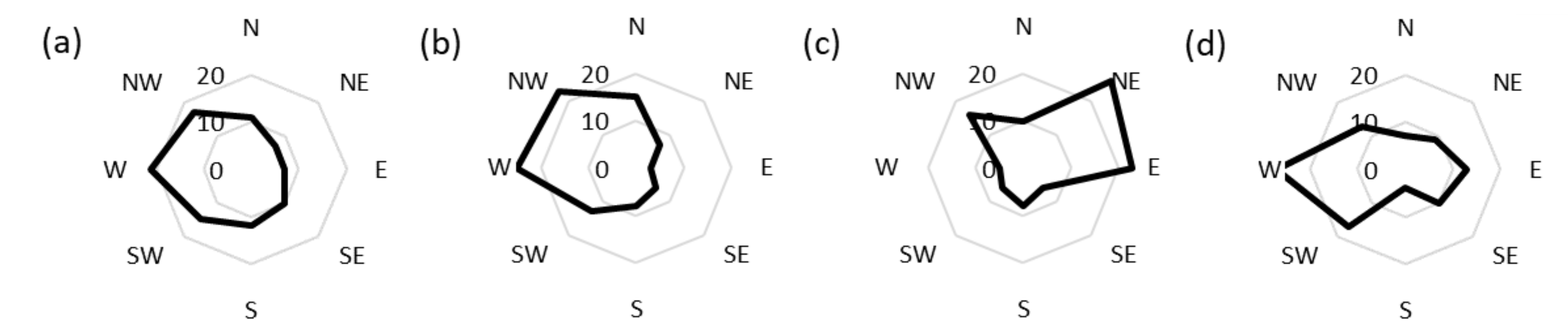
4.5. Tracing of Contamination Hotspots and Presumable Emission Sources via Mapping of gI Values

Taking into account the discussion above, the following 17 analytes are presumed to have at least mixed, i.e., crustal and partially anthropogenic, origin: As, Br, Ca, Cl, Cr, Cu, Fe, K, Mg, Mn, Ni, P, Pb, S, Sr, V, and Zn. Multi-panel figures were prepared for them (Figures S1–S17). Comparison of the distributions of Igeo‘N and Igeo‘C values of different analytes among different SCC is given in Figure 14: the higher the value of n, the better the index for revealing hotspots.
It seems that from two alternative Igeo indices, Igeo‘N was the better choice to reveal hotspots, since respective n values of As, Cl, Cr, Fe, Mg, Mn, Ni, S, Sr, and V were higher, the only exception being Pb. The wider spread (more SCC intervals) of Igeo‘N distribution was determined by lower Bn values than Cv values (Table S2). For example, for Cl, its Bn = 99 µg g−1 and Igeo‘N was distributed among seven SCC intervals, while its Cv = 370 µg g−1 was higher; therefore, Igeo‘C values were found only in five SCC intervals. The aE’N values found in the interval 1–1.5 enabled us to draw attention to K as possible pollutant. Meanwhile, according to Igeo‘N it could remain unnoticed (Figure S8).
The judgement about prevailing natural, mixed or anthropogenic origin of elements according to nEF indices also depended on THR values. If evaluation was according to nEF’Al’C and the lower TRH was 1, while the upper one was 10, five dust sampling sites according to Mg and one according to Cr would be assigned to those having prevailing natural origin (Figure 15). Meanwhile 14 analytes which can be suspected for significant anthropogenic sources can be arranged in the following sequence according to the number of sites where the index exceeds 10: Br, Cu, S, Zn (20 sites for each) > Ca, P (19) > Cl, Pb (18) > Fe (12) > Cr (11) > As (5) > Ni (4) > Sr, K (1). But if we selected the lower THR equal to 10 which was proposed in [40] for attribution to prevailing crustal origin, the number of analytes with such possible origin would increase from aforementioned two to 13. The analytes can be arranged according to decreasing number of such sites as follows: V, Mn, Mg (20 sites for each) > Sr, K (19) > Ni (16) > As (15) > Cr (9) > Fe (8) > Pb, Cl (2) > Ca, P (1). However, if we take into account the upper THR equal to 20 proposed in [40] for judgement about anthropogenic origin, K will be lost from aforementioned list of 14 elements, while another 13 analytes will be arranged according to decreasing number of such sites as follows: Zn (20) > Br (19) > Cu, S (>18) > P (15) > Cl (14) > Fe (11) > Cr (10) > Pb (8) > Ca, As (3) > Sr, Ni (1).
If evaluation of the analyte origin is done according to nEF’Al’N and the lower THR is 1, while the upper THR is 10 (it is the same according to common publications [45,46,47] and publication of Cesari et al. [40]) Mg in four sites and Cr in one site would be attributed to prevailing natural origin. Meanwhile, the analytes suspected for mainly anthropogenic origin would be arranged in the following sequence: Ca, Cu, Zn (20) > Cl, P (19) > S (18) > Fe, Cr (12) > Ni (11) > Br (8) > As (3) > Pb, Sr (2) > V (1). However, if the lower THR equal to 5 proposed in [40] was selected, the number of analytes with prevailing natural origin would be higher and they would be arranged in the following sequence: K (19) > Mg (16) > Mn (13) > Pb (11) > V (8) > Sr (7) > Cr, Fe (5) > Ni, Br (3).
The contrast of each element urban anomalies is characterized by the ratio (RP) of the 75th percentile to 25th percentile of its geochemical index gI. The size (areas) of hotspots and contrast of elemental anomalies is reflected in the following sequence of respective RP ratios of aE’N index: Fe (11.1) > Mg (6.1) > Zn (4.1) > Cr (3.4) > Sr (2.5) > Cl, Ca (2.4) > As (2.3) > Cu, P (2.2) > K (2.0) > Ni, V (1.9) > Pb (1.8) > Br (1.7) > Mn (1.5) > S (1.4). Meanwhile RP ratios of nEF’Al’N reflect relative anthropogenic part of analytes in dust as well as the variety of their presumable emission sources and their uneven distribution in the city. According to these RP ratios, the elements are arranged as follows: Cu (22.1) > Cr (7.8) > Mn (3.3) > K (3.0) > P (2.7) > Sr (2.5) > Zn (1.9) > Pb (1.8) > Fe (1.7) > V, S (1.6) > Br, Ca (1.5) > Ni (1.7) > As, Cl (1.2) > Mg (1.1). These RP ratios could help to perceive the indices presented in Figures S1–S17, to increase the readability of maps, to highlight the main hotspots of analytes enriching dust, and to find out their dominant emission sources. It is obvious that the main source of Fe is iron ore stevedoring, of Mg is dolomite, and of Sr and P is apatite and phosphorite. The anomalies of Cr can be caused by close distance to iron ore stevedoring and dust re-suspended from former topsoil anomaly in the neighborhood. Hotspots of As and Pb are also at close distance. Meanwhile Zn, Cu, Ni, and V are widely spread in all urban territory. The influence of KCl fertilizers stevedoring is slightly visible from K and Cl spread. Therefore, more detailed research of stevedoring sites is necessary in future, i.e., not only near iron ore stevedoring (B site), but also in other stevedoring sites (C, D, E). The spread of S and halogens Br and Cl is scattered. Actually, their hotspots, as well as hotspots of many other analytes (Mn, V, Ni, etc.) can be masked by high content of iron ore stevedoring dust. It is possible that to reduce this masking, other analytes (e.g., Fe, Mn, or Ti) can be used as reference elements or even complex nEF indices. Examples of such attempts have been shown earlier [25,112].

5. Conclusions

Geochemical exploration methods are useful when using total suspended particles (TSP) to detect hotspots of contaminants and their presumable emission sources in the sites with stevedoring operations. The sequential exploration methodology used in port city Klaipėda included: (a) sampling of TSP with original construction passive samplers as well as the characteristic dust of stevedored material, (b) elemental analysis of a large set (22) of analytes including so-called PHEs, crustal elements, and halogens determined by EDXRF with special sample preparation procedures, (c) multivariate statistical analysis (principal component and cluster analysis) of obtained XRF analysis data to reveal groups of syngenetic inter-correlated analytes, (d) search for reasons to explain temporal variability of geochemical composition of TSP during four monitoring periods, and (e) analysis of obtained analytical data using widely applicable geochemical indices and their mathematical treatment as well geochemical mapping. The conclusions are given below.
The TSP in surroundings of iron ore open stevedoring is greatly enriched with Fe. The aureole of increased Fe contents is spreading from this site to the rest part of the city. Iron is accompanied by Cr. Besides, statistical tests and geochemical mapping of normalized enrichment factors show that As, Pb, S, Mn, Br, Cl, V, and Ni anomalies are also in the same area with these two elements. However, part of Cr can be enriched in TSP due to the input from the former pedogeochemical anomaly as a result of re-suspension from topsoil. In dust near this pedogeochemical anomaly, the contents of As and Pb are also increased. The TSP near stevedoring of phosphorite and apatite raw material and production from them is enriched with Sr and P. Part of Ca is also enriched in this TSP. The stevedoring of dolomite is accompanied by obvious TSP enrichment with Mg which is inevitably related with Ca. The TSP in the part of the city at greater distance from iron ore stevedoring is enriched in so-called crustal elements K, Ti, Rb, Al, Si, Zr, Ca, and Mg as a result of their re-suspension from topsoil. These elements mask the influence of stevedoring operations of KCl fertilizers, but insignificant input of K and Cl can be noticed via geochemical mapping of geochemical indices. The direction of the NW–W–SW winds contributes to enrichment of atmosphere not only with industrial long-range transport pollutants, but also with marine and those coming during stevedoring works. Therefore, local emission sources of S and halogens Br and Cl still remain questionable. Increased contents of these elements as well as Zn and other PHEs were determined in waste incineration plant ash. These elements, except Br, are listed in the application for permit for emissions of this company to the ambient air. The question about emission sources of Br is relevant due to lack of attention to this element: researchers discuss it in less than 20% of publications concerning TSP. Rather little attention (<50% of publications) is also payed to Si, Mg, P, Zr, as well as to As, Al, K, S, Sr, Rb, and Cl (<70% of publications). Both our and other research, e.g., the one performed in [82], demonstrate that when greater number of analytes is determined including the so-called crustal elements, the preliminary emission sources of pollutants can be more precisely revealed using multivariate statistical methods.
It is noted that geochemical composition of TSP can be significantly variable in time due to both weather changes and other reasons, e.g., episodic stevedoring. TSP analysis in Klaipėda during four periods has revealed that such significantly variable analytes are Cl, S, Sr, Ni, Br, V, and Zn. Therefore, it is recommended to compare the contents of analytes in different sites only when sampling there is performed at the same time. Other circumstances which limit the comparability of data published by other researchers as well as lack of expedient information are also mentioned in the study. The ratio of 75th percentile and 25th percentile of geochemical indices is proposed for characterization of elemental spread.
Rather great attention is paid to often irresponsible usage of geochemical indices by some authors for dust classification into so-called “contamination classes”, when the data in the denominators of indices are not related to dust analysis. Taking into account the material of this study we dared to propose to refuse from using the term “contamination classes”, if they are distinguished according to geochemical indices of dust. This assignment is related to subjective factor, i.e., when different values are taken in the denominator during calculation of geochemical indices, so manipulations are possible. We propose careful choice of terminology. For example, in the case of Igeo‘N, the term “(top)soil-enrichment Igeo index“, while in case of Igeo‘C—“Clarke-enrichment Igeo index“ or similar alternatives can be used. In our opinion, normalized enrichment factors cannot be used for naming “contamination classes”.

Supplementary Materials

The following are available online at https://www.mdpi.com/article/10.3390/app112311157/s1, Figure S1: Distribution of As via geochemical indices in TSP of Klaipėda, Figure S2: Distribution of Br via geochemical indices in TSP of Klaipėda, Figure S3: Distribution of Ca via geochemical indices in TSP of Klaipėda, Figure S4: Distribution of Cl via geochemical indices in TSP of Klaipėda, Figure S5: Distribution of Cr via geochemical indices in TSP of Klaipėda, Figure S6: Distribution of Cu via geochemical indices in TSP of Klaipėda, Figure S7: Distribution of Fe via geochemical indices in TSP of Klaipėda, Figure S8: Distribution of K via geochemical indices in TSP of Klaipėda, Figure S9: Distribution of Mg via geochemical indices in TSP of Klaipėda, Figure S10: Distribution of Mn via geochemical indices in TSP of Klaipėda, Figure S11: Distribution of Ni via geochemical indices in TSP of Klaipėda, Figure S12: Distribution of P via geochemical indices in TSP of Klaipėda, Figure S13: Distribution of Pb via geochemical indices in TSP of Klaipėda, Figure S14: Distribution of S via geochemical indices in TSP of Klaipėda, Figure S15: Distribution of Sr via geochemical indices in TSP of Klaipėda, Figure S16: Distribution of V via geochemical indices in TSP of Klaipėda, Figure S17: Distribution of Zn via geochemical indices in TSP of Klaipėda, Table S1: Main meteorological data during the TSP sampling periods, Table S2: Elemental contents (µg g1) in dust of port city Klaipėda, Table S3: The 25th and 75th percentiles of this study and reference values of analytes (μg g1) from selected publications, Table S4: Factor loadings of complete datasets of TSP and background topsoil samples, Table S5: Mean elemental contents (μg g−1) and geochemical indices (gI) in Klaipėda dust during four sampling periods, Table S6: Medians of aE’N during study periods P1, P2, P3 and P4 and significance of variability of elemental contents, Table S7: Medians of Igeo’N and aE’N in dust from two areas and differences between the areas in the values of each index, Table S8: Medians of nEF’Al’C and nEF’Al’N in dust from two areas and differences between the areas in the values of each index.

Author Contributions

Conceptualization: P.R. and R.T. formed main ideas for the research; methodology was developed by P.R. and R.T.; statistical calculation and evaluation of results: R.T. and R.Z.; validation: P.R., R.T. and S.S.; taking and preparations of samples a well as sample analysis: N.L., S.S. and R.T.; investigation of sample analysis results: P.R., N.L. and R.T.; resources for research including manufacturing of passive samplers: P.R.; data curation: P.R. and R.T., writing—original draft preparation: P.R., R.T., R.Z., N.L. and S.S.; writing—review and editing: P.R., R.T. and R.Z.; visualization: R.T.; supervision: P.R. and R.T.; project administration: P.R.; funding acquisition for research: P.R. All authors have read and agreed to the published version of the manuscript.

Funding

This research received no external funding.

Institutional Review Board Statement

Not applicable.

Informed Consent Statement

Not applicable.

Data Availability Statement

Not applicable.

Acknowledgments

The authors are grateful to Senior specialist of the Lithuanian Hydrometeorological Service Judita Navašinskienė for providing meteorological data and support for this research. Authors are grateful to The Environmental Protection Agency for providing data, cooperation and support for our research.

Conflicts of Interest

The authors declare no conflict of interest.

References

  1. Lequy, E.; Siemiatycki, J.; Leblond, S.; Meyer, C.; Zhivin, S.; Vienneau, D.; de Hoogh, K.; Goldberg, M.; Zins, M.; Jacquemin, B. Long-term exposure to atmospheric metals assessed by mosses and mortality in France. Environ. Int. 2019, 129, 145–153. [Google Scholar] [CrossRef] [PubMed]
  2. Canha, N.; Almeida, M.; Do Carmo Freitas, M.; Almeida, S.M.; Wolterbeek, H.T. Seasonal variation of total particulate matter and children respiratory diseases at Lisbon primary schools using passive methods. Procedia Environ. Sci. 2011, 4, 170–183. [Google Scholar] [CrossRef] [Green Version]
  3. Rahman, M.S.; Bhuiyan, S.S.; Ahmed, Z.; Saha, N.; Begum, B.A. Characterization and source apportionment of elemental species in PM2.5 with especial emphasis on seasonal variation in the capital city “Dhaka”, Bangladesh. Urban Clim. 2021, 36, 100804. [Google Scholar] [CrossRef]
  4. Lin, Y.-C.; Hsu, S.-C.; Lin, S.-H.; Huang, Y.-T. Metallic elements emitted from industrial sources in Taiwan: Implications for source identification using airborne PM. Atmos. Pollut. Res. 2020, 11, 766–775. [Google Scholar] [CrossRef]
  5. Abbasi, S.; Keshavarzi, B.; Moore, F.; Hopke, P.K.; Kelly, F.J.; Dominguez, A.O. Elemental and magnetic analyses, source identification, and oxidative potential of airborne, passive, and street dust particles in Asaluyeh County, Iran. Sci. Total Environ. 2020, 707, 136132. [Google Scholar] [CrossRef]
  6. Zhao, J.; Zhang, Y.; Wang, T.; Sun, L.; Yang, Z.; Lin, Y.; Chen, Y.; Mao, H. Characterization of PM 2.5 -bound polycyclic aromatic hydrocarbons and their derivatives (nitro-and oxy-PAHs) emissions from two ship engines under different operating conditions. Chemosphere 2019, 225, 43–52. [Google Scholar] [CrossRef]
  7. Wen, J.; Wang, X.; Zhang, Y.; Zhu, H.; Chen, Q.; Tian, Y.; Shi, X.; Shi, G.; Feng, Y. PM2.5 source profiles and relative heavy metal risk of ship emissions: Source samples from diverse ships, engines, and navigation processes. Atmos. Environ. 2018, 191, 55–63. [Google Scholar] [CrossRef]
  8. Amato, F.; Pandolfi, M.; Moreno, T.; Furger, M.; Pey, J.; Alastuey, A.; Bukowiecki, N.; Prevot, A.S.H.; Baltensperger, U.; Querol, X. Sources and variability of inhalable road dust particles in three European cities. Atmos. Environ. 2011, 45, 6777–6787. [Google Scholar] [CrossRef]
  9. Shen, J.; Feng, X.; Zhuang, K.; Lin, T.; Zhang, Y.; Wang, P. Vertical Distribution of Particulates within the Near-Surface Layer of Dry Bulk Port and Influence Mechanism: A Case Study in China. Sustainability 2019, 11, 7135. [Google Scholar] [CrossRef] [Green Version]
  10. EEA. EMEP/EEA Air Pollutant Emission Inventory Guidebook 2019 2.A.5.c Storage, Handling and Transport of Mineral Products; Publications Office of the European Union: Luxembourg, 2019; ISBN 978-92-9480-098-5.
  11. Tume, P.; King, R.; González, E.; Bustamante, G.; Reverter, F.; Roca, N.; Bech, J. Trace element concentrations in schoolyard soils from the port city of Talcahuano, Chile. J. Geochem. Explor. 2014, 147, 229–236. [Google Scholar] [CrossRef]
  12. Davuliene, L.; Jasineviciene, D.; Garbariene, I.; Andriejauskiene, J.; Ulevicius, V.; Bycenkiene, S. Long-term air pollution trend analysis in the South-eastern Baltic region, 1981–2017. Atmos. Res. 2021, 247, 105191. [Google Scholar] [CrossRef]
  13. Zhao, L.; Wang, L.; Tan, J.; Duan, J.; Ma, X.; Zhang, C.; Ji, S.; Qi, M.; Lu, X.H.; Wang, Y.; et al. Changes of chemical composition and source apportionment of PM 2.5 during 2013–2017 in urban Handan, China. Atmos. Environ. 2019, 206, 119–131. [Google Scholar] [CrossRef]
  14. Taraškevičius, R.; Motiejūnaitė, J.; Zinkutė, R.; Eigminienė, A.; Gedminienė, L.; Stankevičius, Ž. Similarities and differences in geochemical distribution patterns in epiphytic lichens and topsoils from kindergarten grounds in Vilnius. J. Geochem. Explor. 2017, 183, 152–165. [Google Scholar] [CrossRef]
  15. Taraškevičius, R.; Zinkutė, R.; Gedminienė, L.; Stankevičius, Ž. Hair geochemical composition of children from Vilnius kindergartens as an indicator of environmental conditions. Environ. Geochem. Health 2018, 40, 1817–1840. [Google Scholar] [CrossRef]
  16. Baltrenas, P.; Fröhner, K.D.; Pranskevičius, M. Investigation of seaport air dustiness and dust spread. J. Environ. Eng. Landsc. Manag. 2007, 15, 15–23. [Google Scholar] [CrossRef]
  17. Baltrenas, P.; Kvasauskas, M.; Frohner, K.D. Influence of stevedoring operations of liquid and powdery fertilizers at klaipeda state seaport on the ambient air quality. J. Environ. Eng. Landsc. Manag. 2006, 14, 59–68. [Google Scholar] [CrossRef]
  18. Zhao, M.; Zhang, Y.; Ma, W.; Fu, Q.; Yang, X.; Li, C.; Zhou, B.; Yu, Q.; Chen, L. Characteristics and ship traffic source identification of air pollutants in China’s largest port. Atmos. Environ. 2013, 64, 277–286. [Google Scholar] [CrossRef]
  19. Taraškevičius, R. Klaipėdos Miesto Ikimokyklinių Įstaigų, Rekreacinių Ir Visuomeninių Teritorijų Dirvožemio Geocheminė Sudėtis Ir Bendras Miesto Teritorijos Ekogeocheminis Vertinimas (Pagal 2006 Ir 2007 M. Tyrimo Rezultatus) Sudarant Žemėlapius. Available online: http://www.monitor.ku.lt/doc/0%20Virselis%202007.pdf (accessed on 10 August 2021).
  20. Milinis, M. Klaipėdiečių Kantrybė Trūko: Juodos Dulkės Skverbiasi į Būstus, Vaikai Ėmė Kosėti. Available online: https://www.delfi.lt/verslas/verslas/klaipedieciu-kantrybe-truko-juodos-dulkes-skverbiasi-i-bustus-vaikai-eme-koseti.d?id=78829483 (accessed on 12 September 2021).
  21. Taraškevičius, R.; Gulbinskas, S. Pedogeochemical accumulating associations of education and learning institutions and sport stadiums in Klaipeda. In Proceedings of the 15th International Conference on Heavy Metals in the Environment, Gdańsk, Poland, 19–23 September 2010; Department of Analytical Chemistry, Chemical Faculty: Gdansk, Poland, 2010; pp. 781–784. [Google Scholar]
  22. Gaidelys, V.; Benetyte, R. Analysis of the Competitiveness of the Performance of Baltic Ports in the Context of Economic Sustainability. Sustainability 2021, 13, 3267. [Google Scholar] [CrossRef]
  23. Climate Data. Available online: https://en.climate-data.org/europe/lithuania/klaipeda-county/klaipeda-432/ (accessed on 21 August 2021).
  24. Bitinas, A.; Damušyte, A. The littorina sea at the Lithuanian maritime region. Pol. Geol. Inst. Spec. Pap. 2004, 11, 37–46. [Google Scholar]
  25. Zinkutė, R.; Taraškevičius, R.; Jankauskaitė, M.; Stankevičius, Ž. Methodological alternatives for calculation of enrichment factors used for assessment of topsoil contamination. J. Soils Sediments 2017, 17, 440–452. [Google Scholar] [CrossRef]
  26. Air Quality. Available online: https://aaa.lrv.lt/lt/veiklos-sritys/oras/oro-kokybes-statistika-ir-duomenys/metu-oro-kokybes-rodikliai (accessed on 15 May 2021).
  27. Van Dijk, D. Wageningen Evaluating Programmes for Analytical Laboratories (Wepal): A World of Experience. Commun. Soil Sci. Plant Anal. 2002, 33, 2457–2465. [Google Scholar] [CrossRef]
  28. Schramm, R.; Heckel, J. Fast analysis of traces and major elements with ED(P)XRF using polarized X-rays: TURBOQUANT. J. Phys. IV 1998, 8, Pr5-335–Pr5-342. [Google Scholar] [CrossRef]
  29. Introducing a New Era in Analytical Performance. Available online: https://www.spectro.com/products/xrf-spectrometer/xepos-xrf-spectrometer (accessed on 15 May 2021).
  30. Analyzing Trace Elements in Pressed Pellets of Geological Materials Using ED-XRF. Available online: https://extranet.spectro.com/-/media/5C512E72-682D-45D8-AE56-6740529341BC.pdf (accessed on 17 November 2021).
  31. Taraškevičius, R.; Zinkutė, R.; Stakėnienė, R.; Radavičius, M. Case Study of the Relationship between Aqua Regia and Real Total Contents of Harmful Trace Elements in Some European Soils. J. Chem. 2013, 2013, 678140. [Google Scholar] [CrossRef] [Green Version]
  32. Rudnick, R.L.; Gao, S. Composition of the Continental Crust. In Treatise on Geochemistry; Elsevier: Amsterdam, The Netherlands, 2003; pp. 1–64. [Google Scholar]
  33. Muller, G. Schwermetalle in den sediments des Rheins-Veranderungen Seitt. Umschan 1979, 79, 778–783. [Google Scholar]
  34. Sager, M.; Chon, H.-T.; Marton, L. Spatial variation of contaminant elements of roadside dust samples from Budapest (Hungary) and Seoul (Republic of Korea), including Pt, Pd and Ir. Environ. Geochem. Health 2015, 37, 181–193. [Google Scholar] [CrossRef]
  35. Alves, C.A.; Vicente, E.D.; Vicente, A.M.P.; Rienda, I.C.; Tomé, M.; Querol, X.; Amato, F. Loadings, chemical patterns and risks of inhalable road dust particles in an Atlantic city in the north of Portugal. Sci. Total Environ. 2020, 737, 139596. [Google Scholar] [CrossRef]
  36. Dytłow, S.; Górka-Kostrubiec, B. Concentration of heavy metals in street dust: An implication of using different geochemical background data in estimating the level of heavy metal pollution. Environ. Geochem. Health 2021, 43, 521–535. [Google Scholar] [CrossRef]
  37. Chen, L.; Zhou, S.; Wu, S.; Wang, C.; He, D. Concentration, fluxes, risks, and sources of heavy metals in atmospheric deposition in the Lihe River watershed, Taihu region, eastern China. Environ. Pollut. 2019, 255, 113301. [Google Scholar] [CrossRef]
  38. Förstner, U.; Müller, G. Concentrations of heavy metals and polycyclic aromatic hydrocarbons in river sediments: Geochemical background, man’s influence and environmental impact. GeoJournal 1981, 5, 417–432. [Google Scholar] [CrossRef]
  39. Rahn, K.A. Sources of Trace Elements in Aerosols: An Approach to Clean Air; U.S. Atomic Energy Commission: Washington, DC, USA, 1971. [Google Scholar] [CrossRef] [Green Version]
  40. Cesari, D.; Contini, D.; Genga, A.; Siciliano, M.; Elefante, C.; Baglivi, F.; Daniele, L. Analysis of raw soils and their re-suspended PM10 fractions: Characterisation of source profiles and enrichment factors. Appl. Geochem. 2012, 27, 1238–1246. [Google Scholar] [CrossRef]
  41. Megido, L.; Negral, L.; Castrillón, L.; Suárez-Peña, B.; Fernández-Nava, Y.; Marañón, E. Enrichment factors to assess the anthropogenic influence on PM10 in Gijón (Spain). Environ. Sci. Pollut. Res. 2017, 24, 711–724. [Google Scholar] [CrossRef] [PubMed]
  42. Švédová, B.; Matýsek, D.; Raclavská, H.; Kucbel, M.; Kantor, P.; Šafář, M.; Raclavský, K. Variation of the chemical composition of street dust in a highly industrialized city in the interval of ten years. J. Environ. Manag. 2020, 267, 110506. [Google Scholar] [CrossRef] [PubMed]
  43. Marín Sanleandro, P.; Sánchez Navarro, A.; Díaz-Pereira, E.; Bautista Zuñiga, F.; Romero Muñoz, M.; Delgado Iniesta, M.J. Assessment of heavy metals and color as indicators of contamination in street dust of a city in SE Spain: Influence of traffic intensity and sampling location. Sustainability 2018, 10, 4105. [Google Scholar] [CrossRef] [Green Version]
  44. Zgłobicki, W.; Telecka, M.; Skupiński, S.; Pasierbińska, A.; Kozieł, M. Assessment of heavy metal contamination levels of street dust in the city of Lublin, E Poland. Environ. Earth Sci. 2018, 77, 774. [Google Scholar] [CrossRef] [Green Version]
  45. Vlasov, D.; Kosheleva, N.; Kasimov, N. Spatial distribution and sources of potentially toxic elements in road dust and its PM10 fraction of Moscow megacity. Sci. Total Environ. 2020, 5, 143267. [Google Scholar] [CrossRef]
  46. Shi, D.; Lu, X. Accumulation degree and source apportionment of trace metals in smaller than 63 μm road dust from the areas with different land uses: A case study of Xi’an, China. Sci. Total Environ. 2018, 636, 1211–1218. [Google Scholar] [CrossRef]
  47. Wang, Q.; Lu, X.; Pan, H. Analysis of heavy metals in the re-suspended road dusts from different functional areas in Xi’an, China. Environ. Sci. Pollut. Res. 2016, 23, 19838–19846. [Google Scholar] [CrossRef]
  48. Gregorauskienė, V.; Taraškevičius, R.; Kadūnas, V.; Radzevičius, A.; Zinkutė, R. Geochemical Characteristics of Lithuanian Urban Areas. In Mapping the Chemical Environment of Urban Areas; John Wiley & Sons, Ltd.: Chichester, UK, 2011; pp. 393–409. [Google Scholar]
  49. Kumpiene, J.; Brännvall, E.; Taraškevičius, R.; Aksamitauskas, Č.; Zinkutė, R. Spatial variability of topsoil contamination with trace elements in preschools in Vilnius, Lithuania. J. Geochem. Explor. 2011, 108, 15–20. [Google Scholar] [CrossRef]
  50. Sajet, J. Geokimija Okrushajuchei Sredi (Environmental Geochemistry); Nedra: Moscow, Russia, 1990. [Google Scholar]
  51. Naraki, H.; Keshavarzi, B.; Zarei, M.; Moore, F.; Abbasi, S.; Kelly, F.J.; Dominguez, A.O.; Jaafarzadeh, N. Urban street dust in the Middle East oldest oil refinery zone: Oxidative potential, source apportionment and health risk assessment of potentially toxic elements. Chemosphere 2021, 268, 128825. [Google Scholar] [CrossRef]
  52. Hakanson, L. An ecological risk index for aquatic pollution control.a sedimentological approach. Water Res. 1980, 14, 975–1001. [Google Scholar] [CrossRef]
  53. Rincheval, M.; Cohen, D.R.; Hemmings, F.A. Biogeochemical mapping of metal contamination from mine tailings using field-portable XRF. Sci. Total Environ. 2019, 662, 404–413. [Google Scholar] [CrossRef]
  54. Castanheiro, A.; Hofman, J.; Nuyts, G.; Joosen, S.; Spassov, S.; Blust, R.; Lenaerts, S.; De Wael, K.; Samson, R. Leaf accumulation of atmospheric dust: Biomagnetic, morphological and elemental evaluation using SEM, ED-XRF and HR-ICP-MS. Atmos. Environ. 2020, 221, 117082. [Google Scholar] [CrossRef]
  55. Peng, L.; Li, X.; Sun, X.; Yang, T.; Zhang, Y.; Gao, Y.; Zhang, X.; Zhao, Y.; He, A.; Zhou, M.; et al. Comprehensive Urumqi screening for potentially toxic metals in soil-dust-plant total environment and evaluation of children’s (0–6 years) risk-based blood lead levels prediction. Chemosphere 2020, 258, 127342. [Google Scholar] [CrossRef]
  56. Huang, J.; Wu, G.; Zhang, X.; Zhang, C. New insights into particle-bound trace elements in surface snow, Eastern Tien Shan, China. Environ. Pollut. 2020, 267, 115272. [Google Scholar] [CrossRef]
  57. Kasimov, N.S.; Vlasov, D.V.; Kosheleva, N.E. Enrichment of road dust particles and adjacent environments with metals and metalloids in eastern Moscow. Urban Clim. 2020, 32, 100638. [Google Scholar] [CrossRef]
  58. Talovskaya, A.V.; Yazikov, E.G.; Osipova, N.A.; Lyapina, E.E.; Litay, V.V.; Metreveli, G.; Kim, J. Mercury Pollution In Snow Cover Around Thermal Power Plants In Cities (Omsk, Kemerovo, Tomsk Regions, Russia). Geogr. Environ. Sustain. 2019, 12, 132–147. [Google Scholar] [CrossRef] [Green Version]
  59. Fujiwara, F.; Rebagliati, R.J.; Marrero, J.; Gómez, D.; Smichowski, P. Antimony as a traffic-related element in size-fractionated road dust samples collected in Buenos Aires. Microchem. J. 2011, 97, 62–67. [Google Scholar] [CrossRef]
  60. Kariper, A.; Üstündağ, İ.; Deniz, K.; Mülazımoğlu, İ.E.; Erdoğan, M.S.; Kadıoğlu, Y.K. Elemental monitoring of street dusts in Konya in Turkey. Microchem. J. 2019, 148, 338–345. [Google Scholar] [CrossRef]
  61. Koh, B.; Kim, E.A. Comparative analysis of urban road dust compositions in relation to their potential human health impacts. Environ. Pollut. 2019, 255, 113156. [Google Scholar] [CrossRef]
  62. Kolakkandi, V.; Sharma, B.; Rana, A.; Dey, S.; Rawat, P.; Sarkar, S. Spatially resolved distribution, sources and health risks of heavy metals in size-fractionated road dust from 57 sites across megacity Kolkata, India. Sci. Total Environ. 2020, 705, 135805. [Google Scholar] [CrossRef]
  63. Lanzerstorfer, C.; Logiewa, A. The upper size limit of the dust samples in road dust heavy metal studies: Benefits of a combined sieving and air classification sample preparation procedure. Environ. Pollut. 2019, 245, 1079–1085. [Google Scholar] [CrossRef]
  64. Urrutia-Goyes, R.; Hernandez, N.; Carrillo-Gamboa, O.; Nigam, K.D.P.; Ornelas-Soto, N. Street dust from a heavily-populated and industrialized city: Evaluation of spatial distribution, origins, pollution, ecological risks and human health repercussions. Ecotoxicol. Environ. Saf. 2018, 159, 198–204. [Google Scholar] [CrossRef]
  65. Cao, L.; Appel, E.; Hu, S.; Ma, M. An economic passive sampling method to detect particulate pollutants using magnetic measurements. Environ. Pollut. 2015, 205, 97–102. [Google Scholar] [CrossRef]
  66. Luo, N.; An, L.; Nara, A.; Yan, X.; Zhao, W. GIS-based multielement source analysis of dustfall in Beijing: A study of 40 major and trace elements. Chemosphere 2016, 152, 123–131. [Google Scholar] [CrossRef]
  67. Wang, J.; Zhang, X.; Yang, Q.; Zhang, K.; Zheng, Y.; Zhou, G. Pollution characteristics of atmospheric dustfall and heavy metals in a typical inland heavy industry city in China. J. Environ. Sci. 2018, 71, 283–291. [Google Scholar] [CrossRef]
  68. Willem Erisman, J.A.N.; Beier, C.; Draaijers, G.; Lindberg, S. Review of deposition monitoring methods. Tellus B Chem. Phys. Meteorol. 1994, 46, 79–93. [Google Scholar] [CrossRef]
  69. Assael, M.J.; Melas, D.; Kakosimos, K.E. Monitoring particulate matter concentrations with passive samplers: Application to the Greater Thessaloniki area. Water Air Soil Pollut. 2010, 211, 395–408. [Google Scholar] [CrossRef]
  70. Abdulaziz, K.; Al-Nadji, K.; Kadri, A.; Kakosimos, K. Airborne particulate matter passive samplers for indoor and outdoor exposure monitoring: Development and Evaluation. In Proceedings of the XIII International Conference on Air Pollution and Control, Paris, France, February 2015; Available online: https://www.researchgate.net/publication/320015014_Airborne_Particulate_Matter_Passive_Samplers_for_Indoor_and_Outdoor_Exposure_Monitoring_Development_and_Evaluation (accessed on 12 September 2021).
  71. García-Florentino, C.; Maguregui, M.; Carrero, J.A.; Morillas, H.; Arana, G.; Madariaga, J.M. Development of a cost effective passive sampler to quantify the particulate matter depositions on building materials over time. J. Clean. Prod. 2020, 268, 122134. [Google Scholar] [CrossRef]
  72. Clarke, F.W. The Relative Abundance of the Chemical Elements. Bull. Philos. Soc. Wash. 1889, 11, 135–143. [Google Scholar]
  73. Soltani, N.; Keshavarzi, B.; Moore, F.; Cave, M.; Sorooshian, A.; Mahmoudi, M.R.; Ahmadi, M.R.; Golshani, R. In vitro bioaccessibility, phase partitioning, and health risk of potentially toxic elements in dust of an iron mining and industrial complex. Ecotoxicol. Environ. Saf. 2021, 212, 111972. [Google Scholar] [CrossRef]
  74. Vehlow, J.; Bergfeldt, B.; Hunsinger, H.; Scifert, H.; Mark, F.E. Bromine in waste incineration partitioning and influence on metal volatilisation. Environ. Sci. Pollut. Res. 2003, 10, 329–334. [Google Scholar] [CrossRef] [PubMed]
  75. Banerjee, A.D.K. Heavy metal levels and solid phase speciation in street dusts of Delhi, India. Environ. Pollut. 2003, 123, 95–105. [Google Scholar] [CrossRef]
  76. Yang, T.; Liu, Q.; Li, H.; Zeng, Q.; Chan, L. Anthropogenic magnetic particles and heavy metals in the road dust: Magnetic identification and its implications. Atmos. Environ. 2010, 44, 1175–1185. [Google Scholar] [CrossRef]
  77. Fakinle, B.S.; Uzodinma, O.B.; Odekanle, E.L.; Sonibare, J.A. Impact of elemental composition of particulate matter in the airshed of a University Farm on the local air quality. Heliyon 2020, 6, e03216. [Google Scholar] [CrossRef]
  78. Goel, V.; Mishra, S.K.; Pal, P.; Ahlawat, A.; Vijayan, N.; Jain, S.; Sharma, C. Influence of chemical aging on physico-chemical properties of mineral dust particles: A case study of 2016 dust storms over Delhi. Environ. Pollut. 2020, 267, 115338. [Google Scholar] [CrossRef]
  79. Ivošević, T.; Mandić, L.; Orlić, I.; Stelcer, E.; Cohen, D.D. Comparison between XRF and IBA techniques in analysis of fine aerosols collected in Rijeka, Croatia. Nucl. Instrum. Methods Phys. Res. Sect. B Beam Interact. Mater. Atoms 2014, 337, 83–89. [Google Scholar] [CrossRef]
  80. Wang, T.; Rovira, J.; Sierra, J.; Chen, S.-J.; Mai, B.-X.; Schuhmacher, M.; Domingo, J.L. Characterization and risk assessment of total suspended particles (TSP) and fine particles (PM2.5) in a rural transformational e-waste recycling region of Southern China. Sci. Total Environ. 2019, 692, 432–440. [Google Scholar] [CrossRef]
  81. Tang, Y.; Han, G. Characteristics of major elements and heavy metals in atmospheric dust in Beijing, China. J. Geochem. Explor. 2017, 176, 114–119. [Google Scholar] [CrossRef]
  82. Vercauteren, J.; Matheeussen, C.; Wauters, E.; Roekens, E.; van Grieken, R.; Krata, A.; Makarovska, Y.; Maenhaut, W.; Chi, X.; Geypens, B. Chemkar PM10: An extensive look at the local differences in chemical composition of PM10 in Flanders, Belgium. Atmos. Environ. 2011, 45, 108–116. [Google Scholar] [CrossRef]
  83. Samek, L.; Stegowski, Z.; Furman, L.; Fiedor, J. Chemical content and estimated sources of fine fraction of particulate matter collected in Krakow. Air Qual. Atmos. Health 2017, 10, 47–52. [Google Scholar] [CrossRef] [Green Version]
  84. Nayebare, S.R.; Aburizaiza, O.S.; Siddique, A.; Carpenter, D.O.; Hussain, M.M.; Zeb, J.; Aburiziza, A.J.; Khwaja, H.A. Ambient air quality in the holy city of Makkah: A source apportionment with elemental enrichment factors (EFs) and factor analysis (PMF). Environ. Pollut. 2018, 243, 1791–1801. [Google Scholar] [CrossRef]
  85. De Vos, W.; Tarvainen, T.; Salminen, R.; Reeder, S.; De Vivo, B.; Demetriades, A.; Pirc, S.; Batista, M.J.; Marsina, K.; Ottesen, R.T.; et al. Geochemical Atlas of Europe. Part 2, Interpretation of Geochemical Maps, Additional Tables, Figures, Maps, and Related Publications; Geological Survey of Finland: Espoo, Finland, 2006; ISBN 9516909566. [Google Scholar]
  86. Shahab, A.; Zhang, H.; Ullah, H.; Rashid, A.; Rad, S.; Li, J.; Xiao, H. Pollution characteristics and toxicity of potentially toxic elements in road dust of a tourist city, Guilin, China: Ecological and health risk assessment. Environ. Pollut. 2020, 266, 115419. [Google Scholar] [CrossRef]
  87. Zinkutė, R.; Taraškevičius, R.; Jankauskaitė, M.; Kazakauskas, V.; Stankevičius, Ž. Influence of site-classification approach on geochemical background values. Open Chem. 2020, 18, 1391–1411. [Google Scholar] [CrossRef]
  88. Reimann, C.; Caritat, P. de Intrinsic Flaws of Element Enrichment Factors (EFs) in Environmental Geochemistry. Environ. Sci. Technol. 2000, 34, 5084–5091. [Google Scholar] [CrossRef]
  89. Reimann, C.; de Caritat, P. Distinguishing between natural and anthropogenic sources for elements in the environment: Regional geochemical surveys versus enrichment factors. Sci. Total Environ. 2005, 337, 91–107. [Google Scholar] [CrossRef]
  90. Ravindra, K.; Mor, S. Variation in Spatial Pattern of Criteria Air Pollutants before and during Initial Rain of Monsoon. Environ. Monit. Assess. 2003, 87, 143–153. [Google Scholar] [CrossRef]
  91. Lee, D.S.; Garland, J.A.; Fox, A.A. Atmospheric concentrations of trace elements in urban areas of the United Kingdom. Atmos. Environ. 1994, 28, 2691–2713. [Google Scholar] [CrossRef]
  92. Kicińska, A.; Bożęcki, P. Metals and mineral phases of dusts collected in different urban parks of Krakow and their impact on the health of city residents. Environ. Geochem. Health 2018, 40, 473–488. [Google Scholar] [CrossRef] [Green Version]
  93. Gunawardana, C.; Goonetilleke, A.; Egodawatta, P.; Dawes, L.; Kokot, S. Source characterisation of road dust based on chemical and mineralogical composition. Chemosphere 2012, 87, 163–170. [Google Scholar] [CrossRef] [Green Version]
  94. Calvo, A.I.; Alves, C.; Castro, A.; Pont, V.; Vicente, A.M.; Fraile, R. Research on aerosol sources and chemical composition: Past, current and emerging issues. Atmos. Res. 2013, 120–121, 1–28. [Google Scholar] [CrossRef]
  95. Baltrėnas, P.; Vaišis, V. Research into soil contamination by heavy metals in the northern part of the Klaipėda city, Lithuania. Geologija 2006, 55, 1–8. [Google Scholar]
  96. Gregorauskienė, V.; Taraškevičius, R. Chromas Klaipėdos dirvožemyje: Kokiais metodais ir kuriose laboratorijose ieškoti. In Proceedings of the Jūros Ir Krantų Tyrimai 2020, Klaipeda, Lithuania, 7–9 October 2020; Klaipėdos Universiteto Jūros Tyrimų Institutas: Klaipeda, Lithuania, 2020; pp. 62–66. [Google Scholar]
  97. Carrero, J.A.; Arrizabalaga, I.; Bustamante, J.; Goienaga, N.; Arana, G.; Madariaga, J.M. Diagnosing the traffic impact on roadside soils through a multianalytical data analysis of the concentration profiles of traffic-related elements. Sci. Total Environ. 2013, 458–460, 427–434. [Google Scholar] [CrossRef]
  98. Caforio, A. Inquinamento atmosferico da piombo. Inquinamento 1986, 28, 54–57. [Google Scholar]
  99. Rakovan, J.F.; Hughes, J.M. Strontium in the Apatite Structure: Strontian Fluorapatite and Belovite-(Ce). Can. Mineral. 2000, 38, 839–845. [Google Scholar] [CrossRef]
  100. Kratz, S.; Schick, J.; Schnug, E. Trace elements in rock phosphates and P containing mineral and organo-mineral fertilizers sold in Germany. Sci. Total Environ. 2016, 542, 1013–1019. [Google Scholar] [CrossRef] [PubMed]
  101. Eurochem Lifosa. Available online: https://www.lifosa.com/en/products-services/production/167 (accessed on 24 May 2021).
  102. Johansson, L.; Jalkanen, J.P.; Kalli, J.; Kukkonen, J. The evolution of shipping emissions and the costs of regulation changes in the northern EU area. Atmos. Chem. Phys. 2013, 13, 11375–11389. [Google Scholar] [CrossRef] [Green Version]
  103. WSY Western Shipyard BLRT Group. Available online: https://wsy.lt/en/ (accessed on 24 May 2021).
  104. Raclavská, H.; Corsaro, A.; Hartmann-Koval, S.; Juchelková, D. Enrichment and distribution of 24 elements within the sub-sieve particle size distribution ranges of fly ash from wastes incinerator plants. J. Environ. Manag. 2017, 203, 1169–1177. [Google Scholar] [CrossRef] [PubMed]
  105. Hopke, P.K.; Dai, Q.; Li, L.; Feng, Y. Global review of recent source apportionments for airborne particulate matter. Sci. Total Environ. 2020, 740, 140091. [Google Scholar] [CrossRef]
  106. Sorte, S.; Rodrigues, V.; Borrego, C.; Monteiro, A. Impact of harbour activities on local air quality: A review. Environ. Pollut. 2020, 257, 113542. [Google Scholar] [CrossRef]
  107. Orlen Lietuva. Available online: https://www.orlenlietuva.lt/EN/Company/OL/Pages/Refinery.aspx (accessed on 24 May 2021).
  108. Crawford, J.; Cohen, D.D.; Chambers, S.D.; Williams, A.G.; Atanacio, A. Impact of aerosols of sea salt origin in a coastal basin: Sydney, Australia. Atmos. Environ. 2019, 207, 52–62. [Google Scholar] [CrossRef]
  109. Rodríguez, S.; Calzolai, G.; Chiari, M.; Nava, S.; García, M.I.; López-Solano, J.; Marrero, C.; López-Darias, J.; Cuevas, E.; Alonso-Pérez, S.; et al. Rapid changes of dust geochemistry in the Saharan Air Layer linked to sources and meteorology. Atmos. Environ. 2020, 223, 117186. [Google Scholar] [CrossRef]
  110. Foltescu, V.L.; Isakson, J.; Sflin, E.; Stikans, M. Measured fluxes of sulphur, chlorine and some anthropogenic metals to the Swedish west coast. Atmos. Environ. 1994, 28, 2639–2649. [Google Scholar] [CrossRef]
  111. Stravinskienė, V. Pollution of “akmenės cementas” vicinity: Alkalizing microelements in soil, composition of vegetation species and projection coverage/”akmenės cemento“ aplinkos tarša. Dirvožemį šarminantys mikroelementai, augalijos rūšių į vairovė ir projekcinis padeng. J. Environ. Eng. Landsc. Manag. 2011, 19, 130–139. [Google Scholar] [CrossRef]
  112. Stančikaitė, M.; Bliujienė, A.; Kisielienė, D.; Mažeika, J.; Taraškevičius, R.; Messal, S.; Szwarczewski, P.; Kusiak, J.; Stakėnienė, R. Population history and palaeoenvironment in the Skomantai archaeological site, West Lithuania: Two thousand years. Quat. Int. 2013, 308–309, 190–204. [Google Scholar] [CrossRef]
Figure 1. Location of TSP sampling sites (their identification number is in the circle) and potential sources of impact in Klaipėda port city. In the port area, the main stevedoring terminals are: A—bulk products loading (fertilizers: KCl, NH4NO3, (NH2)2CO, etc.; grain: wheat, barley, etc.); B—open loading (iron ore, scrap metal, building materials, etc.); C—bulk products loading (cement, apatite, phosphorites, etc.); D—bulk products loading (KCl fertilizers). Other companies and works: E—open warehousing, handling, transportation of granite, dolomite, mineral powder production by rail and trucks; F—waste incineration plant (70-m-high chimney, power plant burns about 255,000 tons per year); FEZ—works of free economic zone (manufacture of electrical installation, PET, HDPE, metal structures, cement packaging etc.); a—oil terminal; b—winter port; c—yacht port; d—ship repair and shipbuilding; e—paper and cardboard factory; f—ferry terminal; g—railway station; h—manufacture of wood products; i—heat, energy production (natural gas, biofuel), j—production and storage of concrete, building mixtures, etc., k—location of former galvanic batteries factory, Cr—anomaly of contaminated topsoil [21]. 1–20 Sampling locations. Ortophoto map layer data: google maps.
Applsci 11 11157 g001
Figure 2. Passive sampler for particulate matter. Roof (1), protective net (2), collection plates (3), fixing bracket (4).
Applsci 11 11157 g002
Figure 3. Comparison of native topsoil background values (Bn) with: Cv—Clarke values [50]; 50th —median elemental contents in dust of the city; elemental contents in stevedored dust of: B’Fe –iron ore; C’ap—apatite; C’ph—phosphorite, D’KCl—potassium fertilizers; F*wa—elemental contents in waste incineration ash.
Applsci 11 11157 g003
Figure 4. Dust particle size in (a) iron ore handling environment (near site B, Figure 1) and (b) in southeastern part of the city (near site E, Figure 1) (b). Arrows highlight non-ferrous crustal (silicate and other) minerals. Photographs were taken using microscope “Nikon Eclipse Ci-L”. The grid was added using software “imageJ”.
Applsci 11 11157 g004
Figure 5. Correspondence of our analysis data to reference values (RV) given in Table S3. The analytes are sorted according to descending frequency of RV within our 25th–75th percentile interval. These frequencies are in white parts of the columns, the frequencies of RV exceeding our 75th percentile are in green parts, while those below our 25th percentiles are in gray parts.
Applsci 11 11157 g005
Figure 6. Frequency of the presence of analytes in reference publications. PHEs are indicated in yellow, crustal elements in brown, halogens in blue.
Applsci 11 11157 g006
Figure 7. Cluster analysis dendrogram of complete dataset of TSP.
Applsci 11 11157 g007
Figure 8. Mean values of Igeo’C and Igeo’N. The analytes are sorted by decreasing Igeo’C values. *—analytes for which so-called contamination classes of alternative indices are different.
Applsci 11 11157 g008
Figure 9. Mean values of nEF’Al’C and nEF’Al’N. The analytes are sorted by decreasing nEF‘Al’C values. *—analytes for which so-called contamination classes of alternative indices are different.
Applsci 11 11157 g009
Figure 10. Median values of aE’N during study periods P1, P2, P3, and P4.
Applsci 11 11157 g010
Figure 11. Rose diagrams of the frequencies (%) of wind directions during study periods P1 (a), P2 (b), P3 (c), and P4 (d).
Applsci 11 11157 g011
Figure 12. Ratios of median elemental aE’N values in two areas. Legend: <1 km/>1 km (in brown) indicates accumulation of analytes in iron ore stevedoring dust in the <1 km area, while >1 km/<1 km (in green) their accumulation in the rest part of the city. The value of ratio is in outline, if U-test shows significant (p < 0.05) difference between the areas in the values of the index.
Applsci 11 11157 g012
Figure 13. Ratios of median elemental nEF’Al’C or nEF’Al’N values in two areas. Explanation of the legend is in Figure 12.
Applsci 11 11157 g013
Figure 14. The frequency distribution of elemental Igeo’N and Igeo’C values of twenty TSP sampling sites in seven so-called contamination classes SCC. Explanation: log2(x) column indicates the threshold values of SCC intervals for logarithmic data, while x column shows respective values for non-logarithmic data. n is the total number of SCC, in which the scatter of occurrences was found.
Applsci 11 11157 g014
Figure 15. The frequency of elemental nEF’Al’C and nEF’Al’N values of twenty TSP sampling sites in three levels indicating possible origin of emission source of analytes. Explanation: mcu are intervals when the thresholds are selected taking into account common publications [45,46,47], crs are those when thresholds suggested in [40] are selected. The red color shows the intervals where the presumable origin of analytes is anthropogenic, green color when it is crustal, while yellow color when it is mixed.
Applsci 11 11157 g015
Publisher’s Note: MDPI stays neutral with regard to jurisdictional claims in published maps and institutional affiliations.

