
Usefulness of Compiled Geophysical Prospecting Surveys in Groundwater Research in the Metropolitan District of Quito in Northern Ecuador


Abstract
1. Introduction
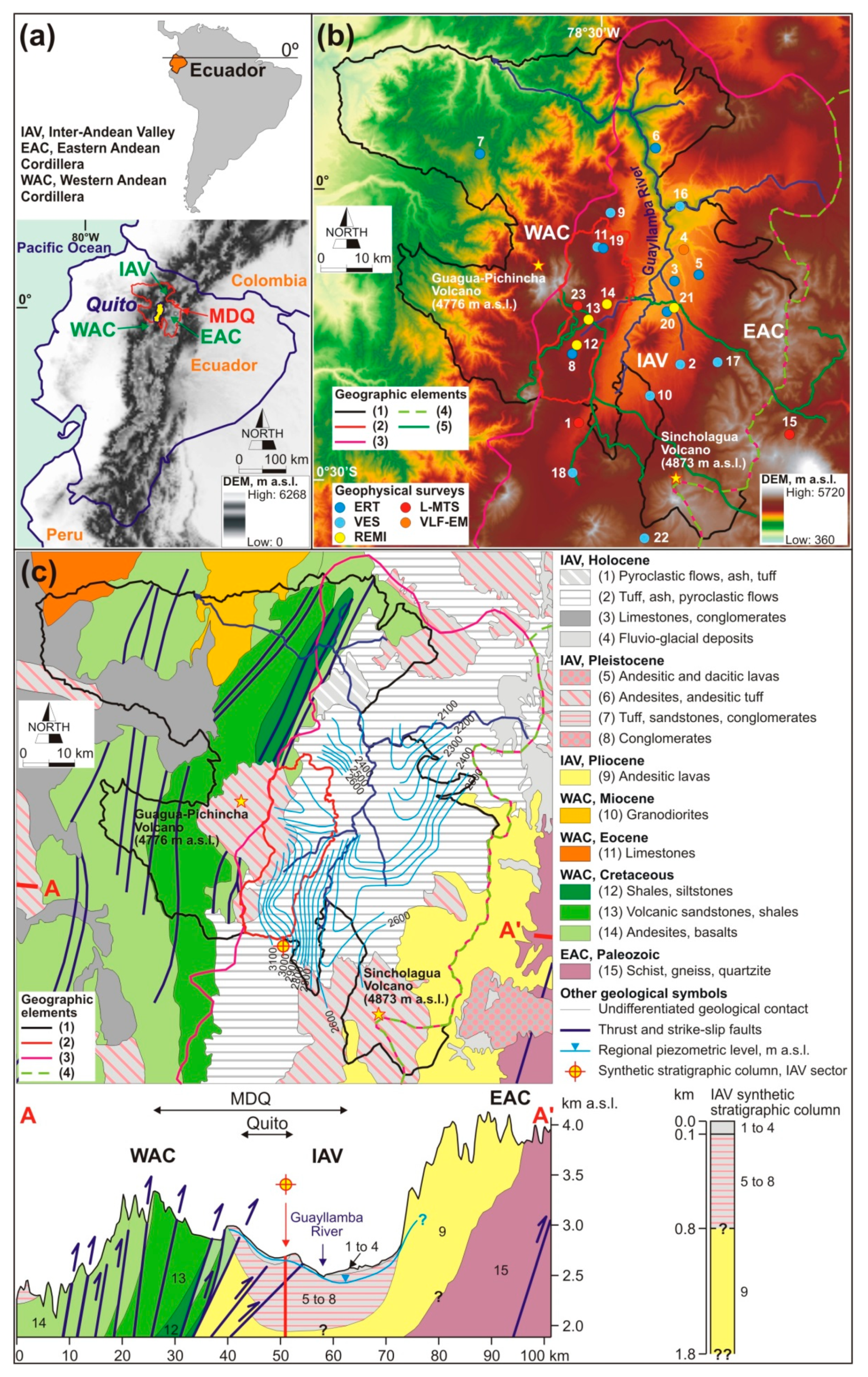
2. Study Area
2.1. Location and Climate
2.2. Geology and Hydrogeology
2.3. Urban Water Demand
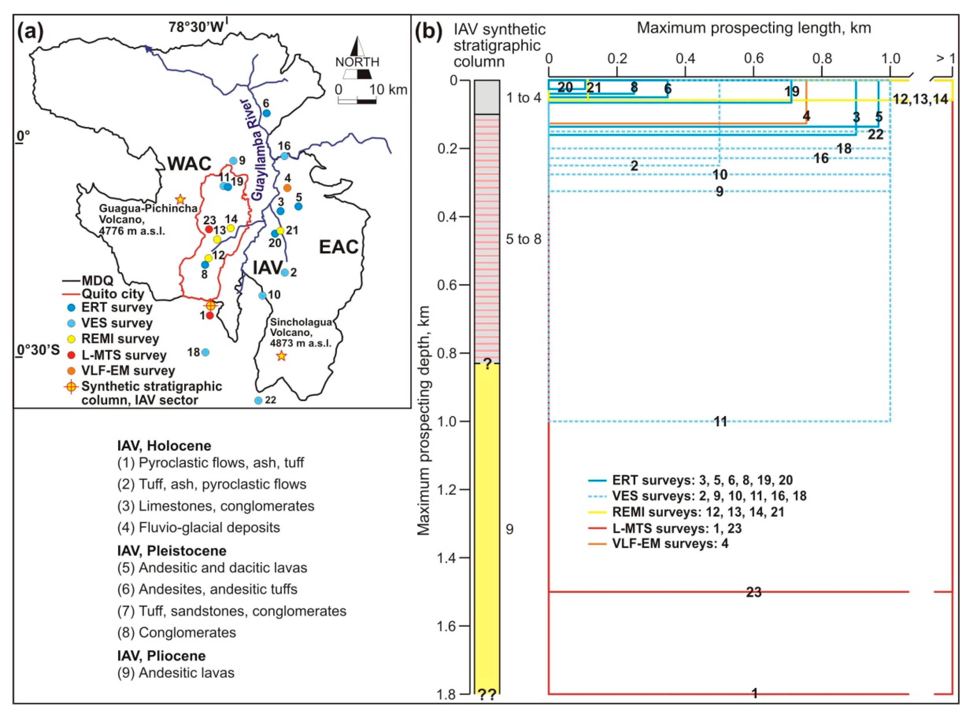
3. Data Compilation
4. Results
4.1. Near-Surface Electrical Surveys
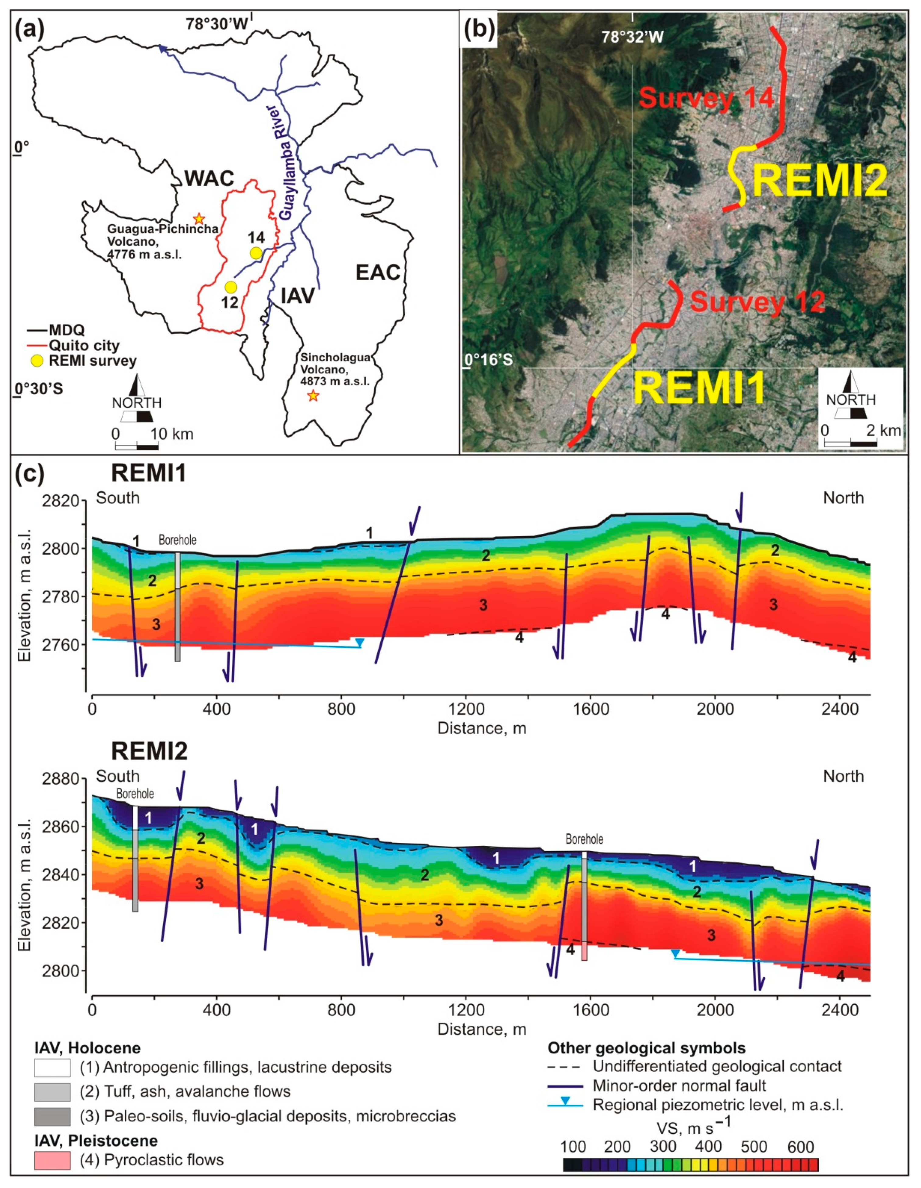
4.2. Near-Surface Seismic Surveys
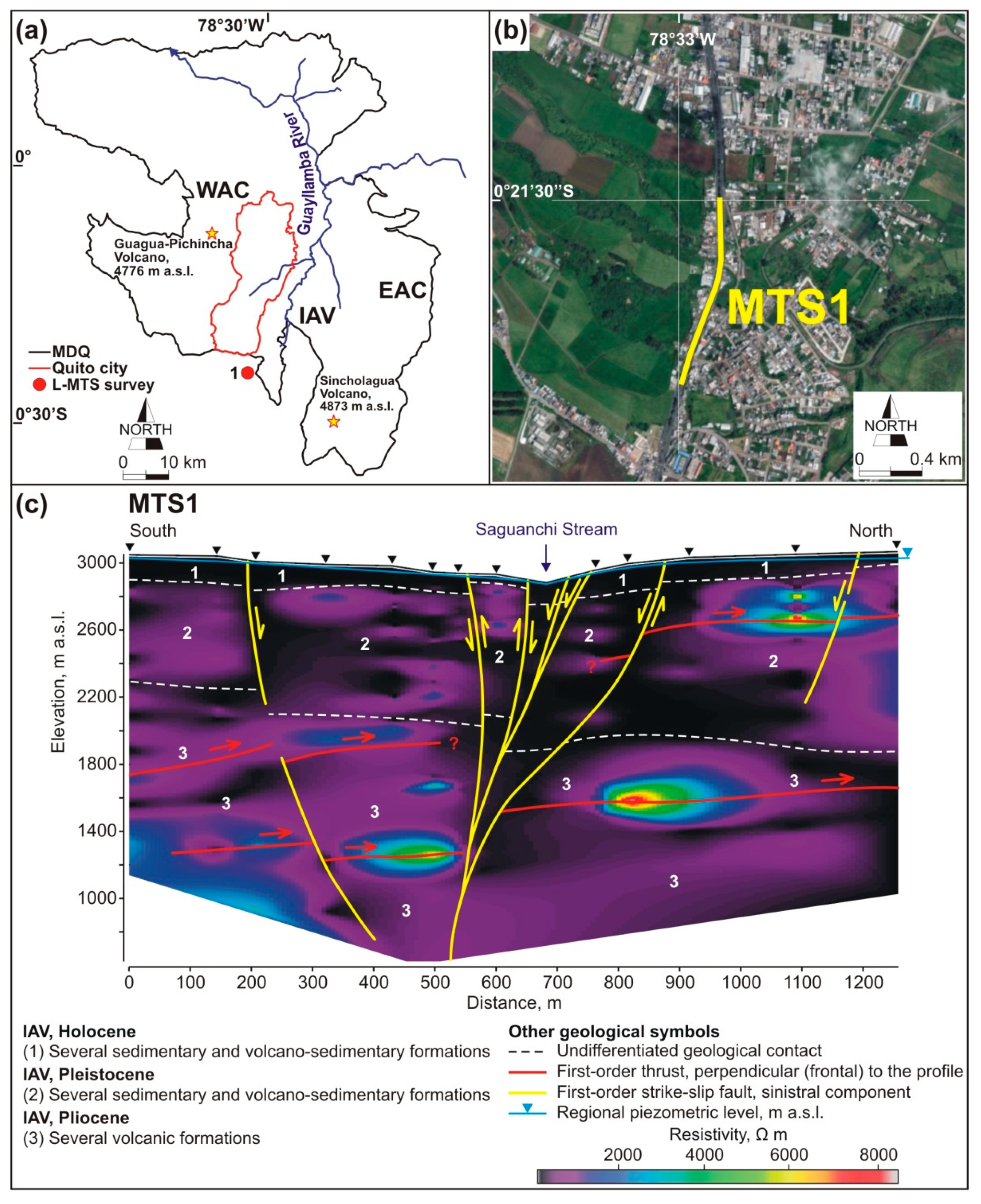
4.3. Electromagnetic Surveys
5. Discussion
6. Conclusions
Author Contributions
Funding
Institutional Review Board Statement
Informed Consent Statement
Data Availability Statement
Acknowledgments
Conflicts of Interest
References
- Barnett, T.P.; Adam, J.C.; Lettenmaier, D.P. Potential impacts of a warming climate on water availability in snow-dominated regions. Nature 2005, 438, 303–309. [Google Scholar] [CrossRef]
- Bradley, R.S.; Vuille, M.; Diaz, H.F.; Vergara, W. Threats to water supplies in the Tropical Andes. Science 2006, 312, 1755–1756. [Google Scholar] [CrossRef] [PubMed]
- Viviroli, D.; Archer, D.R.; Buytaert, W.; Fowler, H.J.; Greenwood, G.B.; Hamlet, A.F.; Huang, Y.; Koboltschning, G.; Litaor, M.L.; López-Moreno, J.L.; et al. Climate change and mountain water resources: Overview and recommendations for research, management and policy. Hydrol. Earth Syst. Sci. 2011, 15, 471–504. [Google Scholar] [CrossRef]
- Buytaert, W.; Célleri, R.; De Bièvre, B.; Cisneros, F.; Wyseure, G.; Deckers, J.; Hofstede, R. Human impact on the hydrology of the Andean páramos. Earth-Sci. Rev. 2006, 79, 53–72. [Google Scholar] [CrossRef]
- Buytaert, W.; Vuille, M.; Dewulf, A.; Urrutia, R.; Karmalkar, A.; Célleri, R. Uncertainties in climate change projections and regional downscaling in the tropical Andes: Implications for water resources management. Hydrol. Earth Syst. Sci. 2010, 14, 1247–1258. [Google Scholar] [CrossRef]
- López, S.; Wright, C.; Costanza, P. Environmental change in the equatorial Andes: Linking climate, land use, and land cover transformations. Remote Sens. 2017, 8, 291–303. [Google Scholar] [CrossRef]
- Flores-López, F.; Galaitsi, S.E.; Escobar, M.; Purkey, D. Modeling of Andean Páramo ecosystems hydrological response to environmental change. Water 2016, 8, 94–111. [Google Scholar] [CrossRef]
- Gonzales-Zeas, D.; Erazo, B.; Lloret, P.; De Biѐvre, D.; Steinchneider, S.; Dangles, O. Linking global climate change to local water availability: Limitations and prospects for a tropical mountain watershed. Sci. Total Environ. 2019, 650, 2577–2586. [Google Scholar] [CrossRef]
- Alcalá, F.J.; Toapanta, J.; Peñafiel, L.; Barragán, E.; Yánez, W.; Buenaño, M.; Larrea, O. First data on atmospheric chloride mass balance components in the Andean páramo in central Ecuador: Implications to project climate scenarios of net aquifer recharge and potential groundwater chemical baseline. In 43rd IAH Congress: Groundwater and Society; IAH: Montpellier, France, 2016; pp. 851–852. [Google Scholar]
- Minga-Leon, S.; Gómez-Albores, M.A.; Bâ, K.M.; Balcázar, L.; Manzano-Solis, L.R.; Cuervo-Robayo, A.P.; Mastachi-Loza, C.A. Estimation of water yield in the hydrographic basin of southern Ecuador. Hydrol. Earth Syst. Sci. Discuss. 2018, Preprint. [Google Scholar] [CrossRef]
- Peñafiel, L.; Alcalá, F.J.; Barragán, E.; Larrea, O. Evaluación del balance hídrico en un área vulcano-sedimentaria de alta montaña poco monitorizada en la Cordillera de los Andes: Acuífero del río Pita, norte de Ecuador. Rev. Lat. Hidrogeol. 2016, 10, 502–508. [Google Scholar]
- Peñafiel, L.; Alcalá, F.J.; Barragán, E.; Toro-Espitia, L.; Larrea, O. Uso de trazadores químicos e isotópicos para deducir el funcionamiento del acuífero del río Pita, Cordillera de los Andes, norte de Ecuador. Rev. Lat. Hidrogeol. 2016, 10, 495–501. [Google Scholar]
- Paz, C.; Alcalá, F.J.; Carvalho, J.M.; Ribeiro, L. Current uses of ground penetrating radar in groundwater-dependent ecosystems research. Sci. Total Environ. 2017, 595, 868–885. [Google Scholar] [CrossRef]
- Monteiro Santos, F.A.; Sultan, S.A.; Represas, P.; El Sorady, A.L. Joint inversion of gravity and geoelectric data for groundwater and structural investigation: Application to the northwestern part of Sinai, Egypt. Geophys. J. Int. 2006, 165, 705–718. [Google Scholar] [CrossRef]
- Alam, K.; Ahmad, N. Determination of aquifer geometry through geophysical methods: A case study from Quetta Valley, Pakistan. Acta Geophys. 2014, 62, 142–163. [Google Scholar] [CrossRef]
- Binley, A.; Hubbard, S.S.; Huisman, J.A.; Revil, A.; Robinson, D.A.; Singha, K.; Slater, L.D. The emergence of hydrogeophysics for improved understanding of subsurface processes over multiple scales. Water Resour. Res. 2015, 51, 3837–3866. [Google Scholar] [CrossRef] [PubMed]
- Uhlemann, S.S.; Sorensen, J.P.R.; House, A.R.; Wilkinson, P.B.; Roberts, C.; Gooddy, D.C.; Binley, A.M.; Chambers, J.E. Integrated time-lapse geoelectrical imaging of wetland hydrological processes. Water Resour. Res. 2016, 52, 3. [Google Scholar] [CrossRef]
- Peñafiel, L.; Reyes, P.S.B.; Alcalá, F.J.; Ramírez, M.R.; Cabero, A. Fold-axis parallel extension along the southern ending of the Quito (Ecuadorian Andes) fault system: Implications in river network and aquifer geometry. Geotectonics 2020, 54, 256–265. [Google Scholar] [CrossRef]
- Bendix, J. Precipitation dynamics in Ecuador and northern Peru during the 1991/92 El Nino: A remote sensing perspective. Int. J. Remote Sens. 2000, 21, 533–548. [Google Scholar] [CrossRef]
- Bendix, J.; Rollenbeck, R.; Palacios, W.E. Cloud detection in the Tropics–a suitable tool for climate-ecological studies in the high mountains of Ecuador. Int. J. Remote Sens. 2004, 25, 4521–4540. [Google Scholar] [CrossRef]
- Van der Hammen, T.; Hooghiemstra, H. Neogene and Quaternary history of vegetation, climate, and plant diversity in Amazonia. Quat. Sci. Rev. 2000, 19, 725–742. [Google Scholar] [CrossRef]
- Garreaud, R.; Falvey, M. The coastal winds off western subtropical South America in future climate scenarios. Int. J. Climatol. 2009, 29, 543–554. [Google Scholar] [CrossRef]
- Rollenbeck, R.; Fabian, P.; Bendix, J. Precipitation dynamics and chemical properties in the mountain forests of Ecuador. Adv. Geosci. 2006, 6, 73–76. [Google Scholar] [CrossRef][Green Version]
- Burbano, N.; Becerra, S.; Pasquel, E. Introduction to the Hydrogeology of Ecuador; Memory and Appendices; National Institute for Meteorology and Hydrology: Quito, Ecuador, 2015; pp. 1–121. [Google Scholar]
- PETROECUADOR. Updated Mapping of Hydrogeological Units and Hydrographic Basins of Ecuador Referenced to the Hydrocarbon Sector Infrastructures (scale 1:1,000,000); Memory and Appendices; Government of Ecuador: Quito, Ecuador, 2005. [Google Scholar]
- EPMAPS. Hydrogeological Map of the Metropolitan District of Quito (scale 1:250,000); International Association of Hydrogeologists-Ecuadorian Group: Quito, Ecuador, 2012; Volume 2, pp. 25–30. [Google Scholar]
- Trenkamp, R.; Kellogg, J.N.; Freymueller, J.T.; Mora, P. Wide plate margin deformation, southern Central America and northwestern South America, CASA GPS observations. J. South Am. Earth Sci. 2002, 15, 157–171. [Google Scholar] [CrossRef]
- Tamay, J.; Galindo-Zaldívar, J.; Ruano, P.; Soto, J.; Lamas, F.; Azañón, J.M. New insight on the recent tectonic evolution and uplift of the southern Ecuadorian Andes from gravity and structural analysis of the Neogene-Quaternary intramontane basins. J. S. Am. Earth Sci. 2016, 70, 340–352. [Google Scholar] [CrossRef]
- Hughes, R.A.; Pilatasig, L.F. Cretaceous and Tertiary terrane accretion in the Cordillera Occidental of the Ecuadorian Andes. Tectonophysics 2002, 345, 29–48. [Google Scholar] [CrossRef]
- Litherland, M.; Aspden, J.; Jemielita, R.A. The Metamorphic Belts of Ecuador. Nottingham; British Geological Survey: Keyworth, UK, 1994; pp. 1–147. [Google Scholar]
- Feininger, T.; Seguin, M.K. Simple Bouguer gravity anomaly field and the inferred crustal structure of continental Ecuador. Geology 1983, 11, 40–44. [Google Scholar] [CrossRef]
- Villagómez, D. Evolución Geológica Plio-Cuaternaria del Valle Interandino Central en Ecuador (Zona de Quito–Guayllabamba–San Antonio). Master’s Thesis, National Polytechnic School, Quito, Ecuador, 2003. [Google Scholar]
- EPMAPS. CAP-1 Borehole Drilling Report: The Pita Aquifer; EPMAPS Repository: Quito, Ecuador, 2016. [Google Scholar]
- EPMAPS. CAP-2 Borehole Drilling Report: The Pita Aquifer; EPMAPS Repository: Quito, Ecuador, 2016. [Google Scholar]
- Muñoz, T. Contributions of Glacier Melting to the Upper Watershed of the Pita River, Ecuador. Master’s Thesis, Michigan Technological University, Houghton, MI, USA, 2016. [Google Scholar]
- Peñafiel, L. Geology and Analysis of the Groundwater Resource in the Southern Quito Subbasin. Master’s Thesis, National Polytechnic School, Quito, Ecuador, 2009. [Google Scholar]
- Larrea, O. Los Acuíferos de Quito, Una Reserva Estratégica; EPMAPS Repository: Quito, Ecuador, 2016. [Google Scholar]
- Vaca, W.; Molano, M.; Heredia, G. Estudio Geológico, Geofísico e Hidráulico en la Zona Industrial de Itulcachi; Memory and Appendices; EPMAPS Repository: Quito, Ecuador, 2012. [Google Scholar]
- Rios-Sanchez, M. A Remote Sensing Approach to Characterize the Hydrogeology of Mountainous Areas: Application to the Quito Aquifer System (QAS), Ecuador. Ph.D. Thesis, Michigan Technological University, Houghton, MI, USA, 2012. [Google Scholar]
- Guachamín, A.; Vaca, W.; Naranjo, F.; Guzmán, G. Elaboración de un Estudio de Tomografías Eléctricas en el Distrito Metropolitano de Quito (DMQ) y Análisis de Conductividades en Pozos; Memory and Appendices; EPMAPS Repository: Quito, Ecuador, 2012. [Google Scholar]
- Guerrero, M. Informe Técnico Agencia Sur del Registro Civil; Secretaría Nacional de Gestión de Riesgos: Quito, Ecuador, 2013; pp. 1–43. [Google Scholar]
- Espinosa, V. Investigaciones de Resistividad Eléctrica en la Exploración de Aguas Subterráneas: Pusuquí-San Antonio y Valle de Los Chillos; Memory and Appendices; EPMAPS Repository: Quito, Ecuador, 2005. [Google Scholar]
- Heredia, H. Investigaciones Hidrogeológicas en el Acuífero de Quito, Sector El Condado; Memory and Appendices; EPMAPS Repository: Quito, Ecuador, 2011. [Google Scholar]
- Cataldi, A. Estudio de Caracterización de Ruta con Métodos Geofísicos no Invasivos: Primera Línea del Metro de Quito; Consorcio GRIFFMETAL–TRX Consulting: Quito, Ecuador, 2011; pp. 1–46. [Google Scholar]
- Beate, B. Estudio de Prefactibilidad Para Elaborar el Modelo Geotérmico Conceptual del Proyecto Chacana; Memory and Appendices; Servicios y Remediación Serviremediación: Quito, Ecuador, 2012; pp. 1–183. [Google Scholar]
- Espinosa, V. Investigaciones Geofísicas de Resistividad Eléctrica en la Exploración de Aguas Subterráneas en el Proyecto El Quinche-Guayllabamba; Memory and Appendices; EPMAPS Repository: Quito, Ecuador, 2007. [Google Scholar]
- Hidalgo, J. Proyecto de Agua Potable Ríos Orientales Portal de Salida del Túnel Papallacta–El Conde: Investigaciones Geofísicas; Memory and Appendices; EPMAPS Repository: Quito, Ecuador, 2005. [Google Scholar]
- Torres, A. Actualización de Los Diseños del Proyecto de Agua Potable Tesalia; Memory and Appendices; EPMAPS Repository: Quito, Ecuador, 2005. [Google Scholar]
- Yautibug, G.; Herrera, F. Investigaciones Mediante Métodos Geofísicos en la Avenida Córdova Galarza; Memory and Appendices; EPMAPS Repository: Quito, Ecuador, 2016. [Google Scholar]
- Vendramini, M.; Bermúdez, R.; Nionelli, P.; Erazo, M. Diseño Definitivo Línea de Transmisión Paluguillo -Bellavista; Memory and Appendices; EPMAPS Repository: Quito, Ecuador, 2017. [Google Scholar]
- Beltrán, E. Estudios de Prospección Geofísica Mediante Sondeos Eléctricos Verticales Realizados en la Cuenca Alta del Río Pita, Provincia de Pichincha; Memory and Appendices; EPMAPS Repository: Quito, Ecuador, 2006. [Google Scholar]
- Reyes, P.S.B.; Ramírez, M.R.; Cajas, M.I. Detecting a master thrust system by magnetotelluric sounding along the western Andean Piedmont of Quito, Ecuador. Terra Nova 2020, 32, 458–467. [Google Scholar] [CrossRef]
- Hayley, K.; Bentley, L.R.; Gharibi, M.; Nightingale, M. Low temperature dependence of electrical resistivity: Implications for near surface geophysical monitoring. Geophys. Res. Lett. 2007, 34, L18402. [Google Scholar] [CrossRef]
- Steelman, C.M.; Kennedy, C.S.; Capes, D.C.; Parker, B.L. Electrical resistivity dynamics beneath a fractured sedimentary bedrock riverbed in response to temperature and groundwater–surface water exchange. Hydrol. Earth Syst. Sci. 2017, 21, 3105–3123. [Google Scholar] [CrossRef]
- Telford, W.M.; Geldart, L.P.; Sheriff, R.E. Applied Geophysics, 2nd ed.; Cambridge University Press: New York, NY, USA, 1990. [Google Scholar]
- Ward, S.H. Resistivity and Induced Polarization Methods. In Geotechnical and Environmental Geophysics, 2nd ed.; Ward, S.H., Ed.; Society of Exploration Geophysicists: Tulsa, OK, USA, 1990; pp. 147–190. [Google Scholar]
- Xia, J.; Miller, R.D.; Park, C.B. Estimation of near-surface shear-wave velocity by inversion of Rayleigh wave. Geophysics 1999, 64, 691–700. [Google Scholar] [CrossRef]
- Xia, J.; Miller, R.D.; Park, C.B.; Hunter, J.A.; Harris, J.B.; Ivanov, J. Comparing shear-wave velocity profiles inverted from multichannel surface wave with borehole measurements. Soil Dyn. Earthq. Eng. 2002, 22, 181–190. [Google Scholar] [CrossRef]
- Park, C.B.; Miller, R.D.; Xia, J. Multi-channel analysis of surface waves. Geophysics 1999, 64, 800–808. [Google Scholar] [CrossRef]
- Park, C.B.; Miller, R.D.; Xia, J.; Ivanov, J. Multichannel analysis of surface waves (MASW)—Active and passive methods. Lead Edge 2007, 26, 60–64. [Google Scholar] [CrossRef]
- Louie, J. Faster, better: Shear-wave velocity to 100 meters depth from refraction microtremor arrays. Bull Seismol. Soc. Am. 2001, 91, 347–364. [Google Scholar] [CrossRef]
- Raines, M.G.; Gunn, D.A.; Morgan, D.J.R.; Williams, G.; Williams, J.D.O.; Caunt, S. Refraction microtremor (ReMi) to determine the shear-wave velocity structure of the near surface and its application to aid detection of a backfilled mineshaft. Q. J. Eng. Geol. Hydrogeol. 2011, 44, 211–220. [Google Scholar] [CrossRef]
- Paz, M.C.; Alcalá, F.J.; Medeiros, A.; Martínez-Pagán, P.; Pérez-Cuevas, J.; Ribeiro, L. Integrated MASW and ERT imaging for geological definition of an unconfined alluvial aquifer sustaining a coastal groundwater-dependent ecosystem in southwest Portugal. Appl. Sci. 2020, 10, 5905. [Google Scholar] [CrossRef]
- Alcalá, F.J.; Martínez-Pagán, P.; Paz, M.C.; Navarro, M.; Pérez-Cuevas, J.; Domingo, F. Combining of MASW and GPR Imaging and Hydrogeological Surveys for the Groundwater Resource Evaluation in a Coastal Urban Area in Southern Spain. Appl. Sci. 2021, 11, 3154. [Google Scholar] [CrossRef]
- García-Jerez, A.; Navarro, M.; Alcalá, F.J.; Luzón, F.; Pérez-Ruiz, J.A.; Enomoto, T.; Vidal, F.; Ocaña, E. Shallow velocity structure using joint inversion of array and h/v spectral ratio of ambient noise: The case of Mula town (SE of Spain). Soil Dyn. Earthq. Eng. 2007, 27, 907–919. [Google Scholar] [CrossRef]
- Mitchell, J.K.; Soga, K. Fundamentals of Soil Behaviour, 3rd ed.; Wiley: London, UK, 2005; pp. 1–592. [Google Scholar]
- Zimmer, M.A.; Prasad, M.; Mavko, G.; Nur, A. Seismic velocities of unconsolidated sands: Part 1—Pressure trends from 0.1 to 20 MPa. Geophysics 2007, 72, E1–E13. [Google Scholar] [CrossRef]
- McGann, C.R.; Bradley, B.A.; Cubrinovski, M. Investigation of shear wave velocity depth variability, site classification, and liquefaction vulnerability identification using a near-surface Vs model of Christchurch, New Zealand. Soil Dyn. Earthq. Eng. 2017, 92, 692–705. [Google Scholar] [CrossRef]
- Alcalá, F.J.; Espinosa, J.; Navarro, M.; Sánchez, F.J. Propuesta de división geológica de la localidad de Adra (provincia de Almería). Aplicación a la zonación sísmica. Rev. Soc. Geológica España 2002, 15, 55–66. [Google Scholar]
- Martínez-Pagán, P.; Navarro, M.; Pérez-Cuevas, J.; Alcalá, F.J.; García-Jerez, A.; Sandoval-Castaño, S. Shear-wave velocity based seismic microzonation of Lorca city (SE Spain) from MASW analysis. Near Surf. Geophys. 2014, 12, 739–749. [Google Scholar] [CrossRef]
- Martínez-Pagán, P.; Navarro, M.; Pérez-Cuevas, J.; Alcalá, F.J.; García-Jerez, A.; Vidal, F. Shear-wave velocity structure from MASW and SPAC methods. The case of Adra town, SE Spain. Near Surf. Geophys. 2018, 16, 356–371. [Google Scholar] [CrossRef]
- Vanorio, T.; Prasad, M.; Patella, D.; Nur, A. Ultrasonic velocity measurements in volcanic rocks: Correlation with microtexture. Geophys. J. Int. 2002, 149, 22–36. [Google Scholar] [CrossRef]
- Unsworth, M.; Soyer, W.; Tuncer, V.; Wagner, A.; Barnes, D. Hydrogeologic assessment of the Amchitka Island nuclear test site (Alaska) with magnetotellurics. Geophysics 2007, 72, B47–B57. [Google Scholar] [CrossRef]
- Chave, A.D.; Jones, A.G. The Magnetotelluric Method: Theory and Practice; Cambridge University Press: New York, NY, USA, 2012; pp. 1–584. [Google Scholar]
- McPhee, D.K.; Chuchel, B.A.; Pellerin, L. Audiomagnetotelluric Data from Spring, Cave, and Coyote Spring Valleys, Nevada; No. 2006-1164; US Geological Survey: Menlo Park, CA, USA, 2006; pp. 1–43. [Google Scholar]
- Zonge, K.L.; Hughes, L.J. Controlled source audio-frequency magnetotellurics. In Electromagnetic Methods in Applied Geophysics, Volume 2: Application, Parts A and B; Nabighian, M.N., Ed.; Society of Exploration Geophysics: McLean, VA, USA, 1991; pp. 713–810. [Google Scholar]
- Geometrics, Inc. Operation Manual for Stratagem Systems Running IMAGEM Ver. 2.19; Geometrics, Inc.: San Jose, CA, USA, 2007. [Google Scholar]
- Buytaert, W.; De Bièvre, B. Water for cities: The impacts of climate change and demographic growth in the tropical Andes. Water Resour. Res. 2012, 48, W08503. [Google Scholar] [CrossRef]


| Lithology | Age | MDQ Sector 1 | Permeability 2 | Effective Porosity 3 | Reference | |
|---|---|---|---|---|---|---|
| Magnitude | Type | |||||
| Metapelites | Paleozoic | EAC | 10−4–10−2 (nd) | fr,fi | nd | [25,26] |
| Andesites and basalts | Cretaceous | WAC | 10−4–10−2 (nd) | fr,fi | nd | [25] |
| Sandstones and siltstones | Cretaceous | WAC | 10−2–10−1 (nd) | fr,fi | nd | [25] |
| Andesitic lavas | early Pleistocene | IAV | 10−2–10−1 (0.04) | fr,fi | nd | [26] |
| Andesitic lavas | middle Pleistocene | IAV | 10−2–10−1 (0.04) | fr,fi | 0.02–0.08 | [26,33,34] |
| Pyroclastic flows | middle Pleistocene | IAV | 0.13–0.86 (nd) | fr,fi | nd | [25,26] |
| Ash | middle Pleistocene | IAV | 10−3–10−1 (0.01) | fr,fi | nd | [25,26] |
| Ash | late Pleistocene | IAV | 10−3–10−1 (0.01) | fr,fi | ˂0.01 | [26,33,34] |
| Fluvio-glacial deposits | late Pleistocene | IAV | 0.05–10 (1.02) | fi,ip | 0.01–0.03 | [25,26] |
| Ash | Holocene | IAV | 10−3–10−1 (nd) | fr,fi | nd | [25,26] |
| Avalanche flows | Holocene | IAV | 10−2–10−1 (nd) | fr,fi | nd | [25,26] |
| Lahar | Holocene | IAV | 10−3–10−2 (0.01) | fr,fi | 0.01–0.06 | [26,33,34] |
| Alluvial | Holocene | IAV | 0.05–0.18 (0.12) | ip | 0.05–0.12 | [25,26] |
| Glacier and moraines | Holocene | IAV | 0.05–0.15 (0.09) | ip | 0.05–0.15 | [25,26] |
| ID | Coordinates | Elevation, m a.s.l. | Geophysical Technique 1 | Geological Environment 2 | Research Interest 3 | Additional Technical Information 4 | Reference | |||||||||||||||
|---|---|---|---|---|---|---|---|---|---|---|---|---|---|---|---|---|---|---|---|---|---|---|
| T1 | T2 | T3 | G1 | G2 | G3 | G4 | G5 | G6 | R1 | R2 | R3 | Variable | AQF | AQT | Profiles | PL | PD | |||||
| 1 | 78°32′ W | 0°24′ S | 3046 | b | a,b | a,b,c | a,b,c | c | a | a,b | b | a | ER, Ω m | 10–210 | 220–8010 | 1 | 1300 | 1800 | [18] | |||
| 2 | 78°22′ W | 0°18′ S | 2644 | a | a,b | a,b | a,b,c | a | a | b | b | ER, Ω m | 62–170 | 10 | 400–500 | 250 | [38] | |||||
| 3 | 78°22′ W | 0°09′ S | 2379 | b | b | a,b,c | a,b,c | a | a | b | b | ER, Ω m | 80–150 | 7 | 504–855 | 70–160 | [39] | |||||
| 4 | 78°21′ W | 0°06′ S | 2350 | a | b | a,b,c | a,b,c | a | a | b | b | ER, Ω m | 15–195 | 210–280 | 13 | 160–750 | 130 | [39] | ||||
| 5 | 78°20′ W | 0°09′ S | 2484 | b | b | a,b,c | a,b,c | a | a | b | a,b | ER, Ω m | 30–75 | 210–250 | 2 | 880 | 137 | [40] | ||||
| 6 | 78°24′ W | 0°04′ N | 2064 | b | b | a,b,c | b,c | a | a,b | a | a,b | ER, Ω m | 10–50 | 2 | 303–358 | 50 | [40] | |||||
| 7 | 78°42′ W | 0°03′ N | 1823 | b | a,b | a,b | b,c | a | a | a | a,b | ER, Ω m | 17–198 | 210–315 | 1 | 715 | 120 | [40] | ||||
| 8 | 78°33′ W | 0°17′ S | 2860 | b | a,b | a,b,c | a,b | a | a | c | ER, Ω m | 3–210 | 215–300 | 9 | 250 | 40 | [41] | |||||
| 9 | 78°29′ W | 0°00′ N | 2736 | a | a,b | a,b | b,c | c | a | b | a | ER, Ω m | 20–40 | 9 | 600–1000 | 322 | [42] | |||||
| 10 | 78°25′ W | 0°21′ S | 2690 | a | a | a,b,c | a,b,c | a | a | a,b | ER, Ω m | 17–28 | 215–345 | 9 | 600–1000 | 271 | [42] | |||||
| 11 | 78°30′ W | 0°06′ S | 2722 | a | a,b | a,b,c | a,b,c | a,b,c | b | b | a,b | ER, Ω m | 30–98 | 11 | 400–1000 | 200–500 | [43] | |||||
| 12 | 78°32′ W | 0°16′ S | 2849 | a | a,b | a,b,c | a,b,c | a | a | c | VS, m s–1 | 95–680 | 95–680 | 171 | 8600 | 40–55 | [44] | |||||
| 13 | 78°31′ W | 0°13′ S | 2826 | a | a,b | a,b,c | c | b | b | c | VS, m s–1 | 135–1050 | 135–1050 | 15 | 3200 | 120 | [44] | |||||
| 14 | 78°29′ W | 0°12′ S | 2777 | a | a,b | a,b,c | a,b,c | a | b | c | VS, m s–1 | 125–710 | 125–710 | 171 | 10,330 | 40–55 | [44] | |||||
| 15 | 78°11′ W | 0°25′ S | 4184 | b | a,b | c | c | a | b | b | b | d | ER, Ω m | 30–215 | 230–3190 | 130 | 15,000 | 4000 | [45] | |||
| 16 | 78°22′ W | 0°02′ S | 2145 | a | a | a,b,c | a | a | b | a | ER, Ω m | 50–170 | 218–457 | 23 | 600–1000 | 230 | [46] | |||||
| 17 | 78°18′ W | 0°18′ S | 3260 | a | a | a,b | c | c | a | b | b | a | ER, Ω m | 28–56 | 3 | 600–800 | 180 | [47] | ||||
| 18 | 78°33′ W | 0°29′ S | 2835 | a | a,b | a,b,c | a | a,b,c | a | b | b | b | ER, Ω m | 45–150 | 255–400 | 16 | 1000 | 200 | [48] | |||
| 19 | 78°29′ W | 0°06′ S | 2693 | b | a,b | a,b | a,b | a | a | a,b | ER, Ω m | 40–100 | 220–320 | 3 | 715 | 60 | [49] | |||||
| 20 | 78°22′ W | 0°12′ S | 2280 | b | a | a,b,c | a | a | c | ER, Ω m | 20–150 | 3 | 110 | 25 | [50] | |||||||
| 21 | 78°22′ W | 0°12′ S | 2400 | a | a | a,b,c | a | a | c | VS, m s–1 | 720–945 | 7 | 120 | 60 | [50] | |||||||
| 22 | 78°25′ W | 0°35′ S | 3743 | a | a,b,c | c | a | b | a | a | ER, Ω m | 56–203 | 225–850 | 20 | 1000 | 150 | [51] | |||||
| 23 | 78°30′ W | 0°12′ S | 2800 | b | a | a,b,c | b,c | c | a | a | b | b | a | ER, Ω m | 22–230 | 235–27,100 | 3 | 17,000 | 1500 | [52] | ||
Publisher’s Note: MDPI stays neutral with regard to jurisdictional claims in published maps and institutional affiliations. |
© 2021 by the authors. Licensee MDPI, Basel, Switzerland. This article is an open access article distributed under the terms and conditions of the Creative Commons Attribution (CC BY) license (https://creativecommons.org/licenses/by/4.0/).
Share and Cite
Peñafiel, L.; Alcalá, F.J.; Senent-Aparicio, J. Usefulness of Compiled Geophysical Prospecting Surveys in Groundwater Research in the Metropolitan District of Quito in Northern Ecuador. Appl. Sci. 2021, 11, 11144. https://doi.org/10.3390/app112311144
Peñafiel L, Alcalá FJ, Senent-Aparicio J. Usefulness of Compiled Geophysical Prospecting Surveys in Groundwater Research in the Metropolitan District of Quito in Northern Ecuador. Applied Sciences. 2021; 11(23):11144. https://doi.org/10.3390/app112311144
Chicago/Turabian StylePeñafiel, Lilia, Francisco Javier Alcalá, and Javier Senent-Aparicio. 2021. "Usefulness of Compiled Geophysical Prospecting Surveys in Groundwater Research in the Metropolitan District of Quito in Northern Ecuador" Applied Sciences 11, no. 23: 11144. https://doi.org/10.3390/app112311144
APA StylePeñafiel, L., Alcalá, F. J., & Senent-Aparicio, J. (2021). Usefulness of Compiled Geophysical Prospecting Surveys in Groundwater Research in the Metropolitan District of Quito in Northern Ecuador. Applied Sciences, 11(23), 11144. https://doi.org/10.3390/app112311144