
Underexposed Vision-Based Sensors’ Image Enhancement for Feature Identification in Close-Range Photogrammetry and Structural Health Monitoring


Abstract
:Featured Application
Abstract
1. Introduction
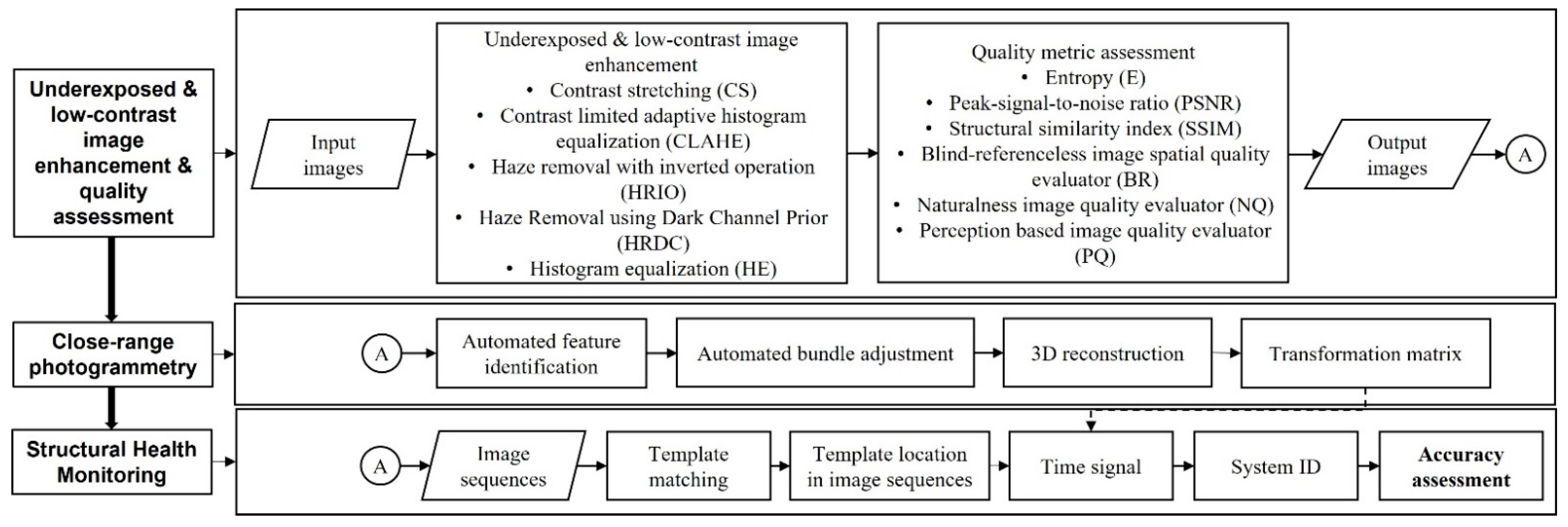
2. Methods
2.1. Feature Detection Problems in Low-Light Setting and Dark Environment
2.2. Image Enhancement Algorithms
2.3. Image Quality Assessment
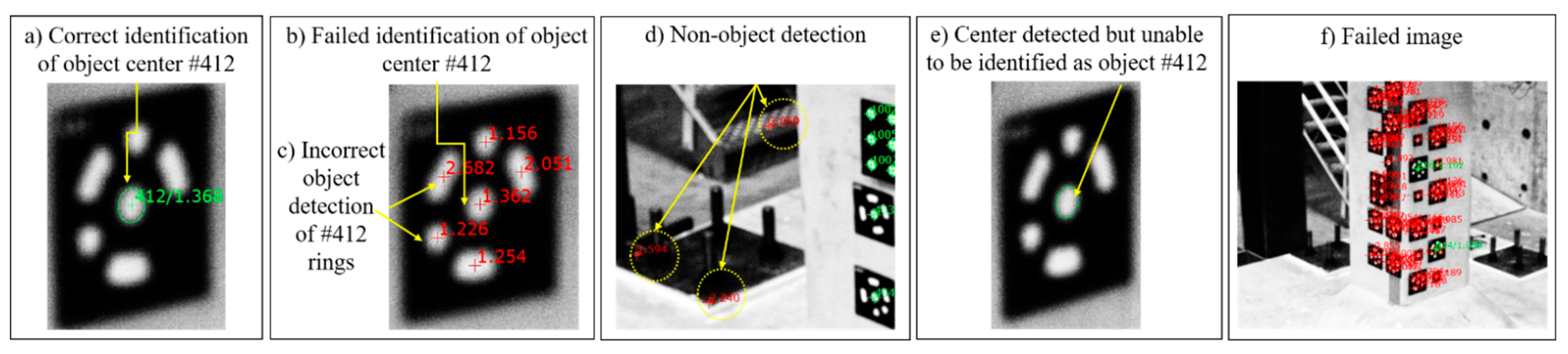
2.4. Automated Identification of Object Features and Significance in Close-Range Photogrammetry and SHM Procedures
3. Implementation and Validation of the Proposed Framework through a One-Inch Block Experiment
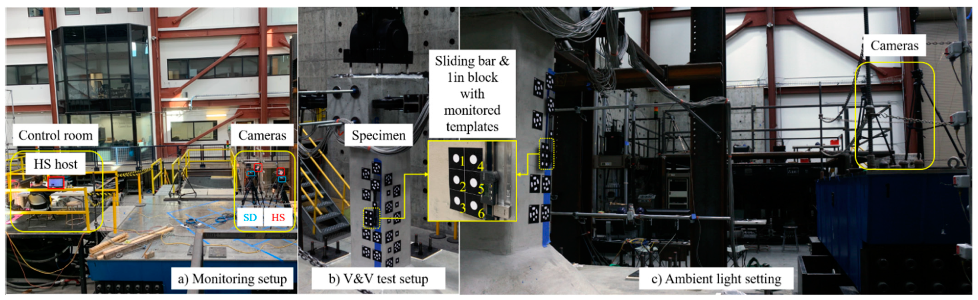
3.1. Experimental Setup
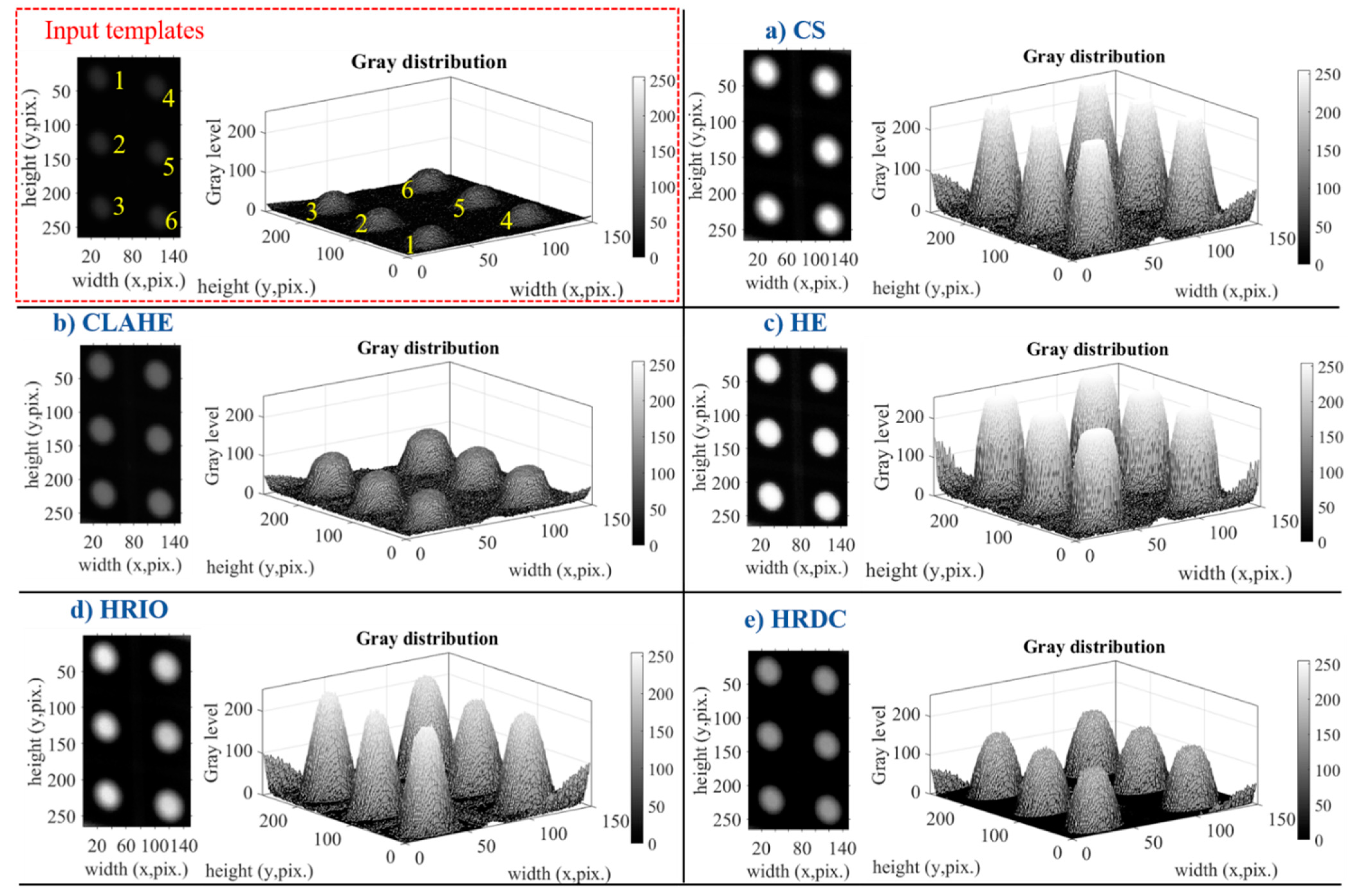
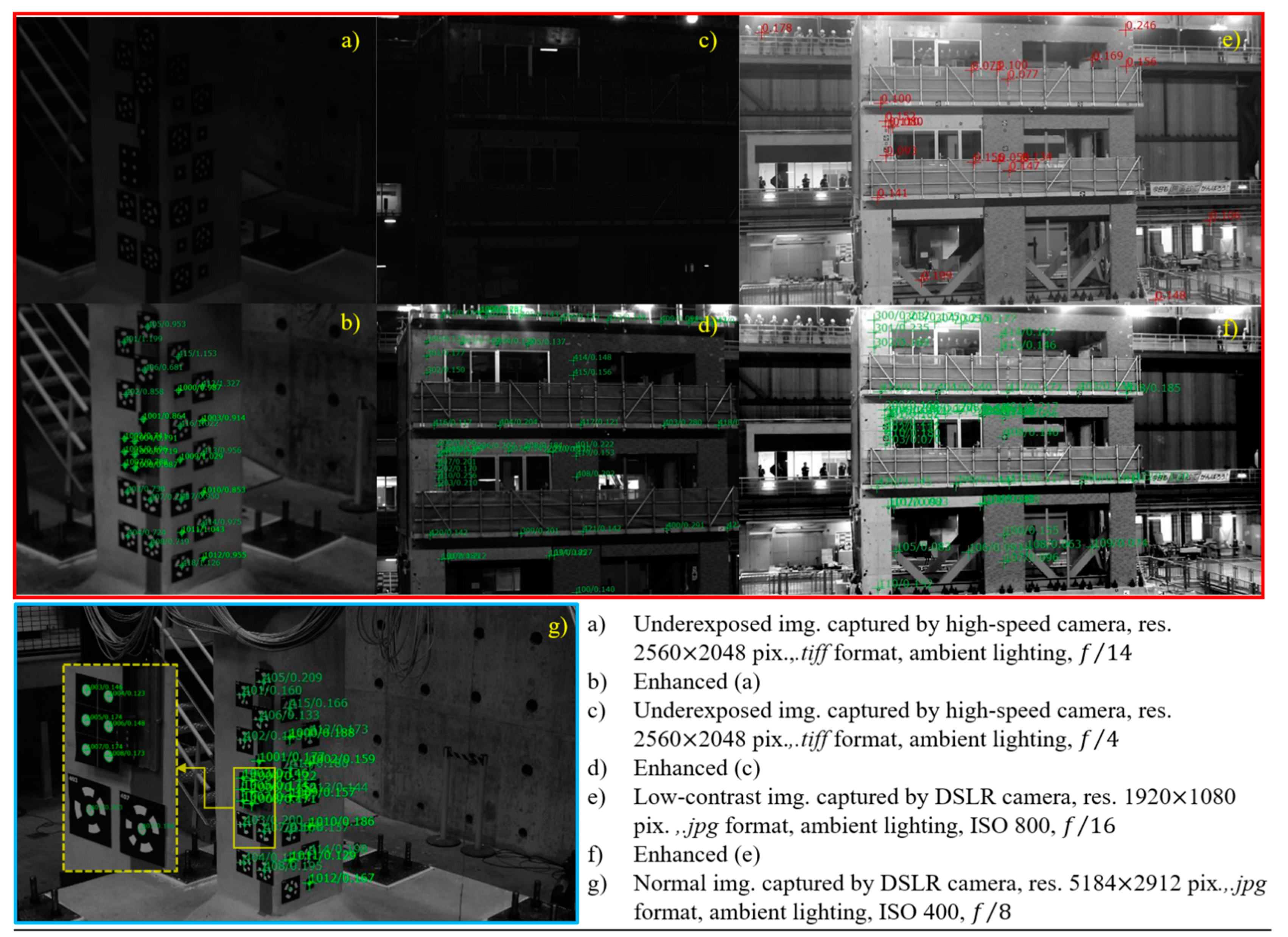
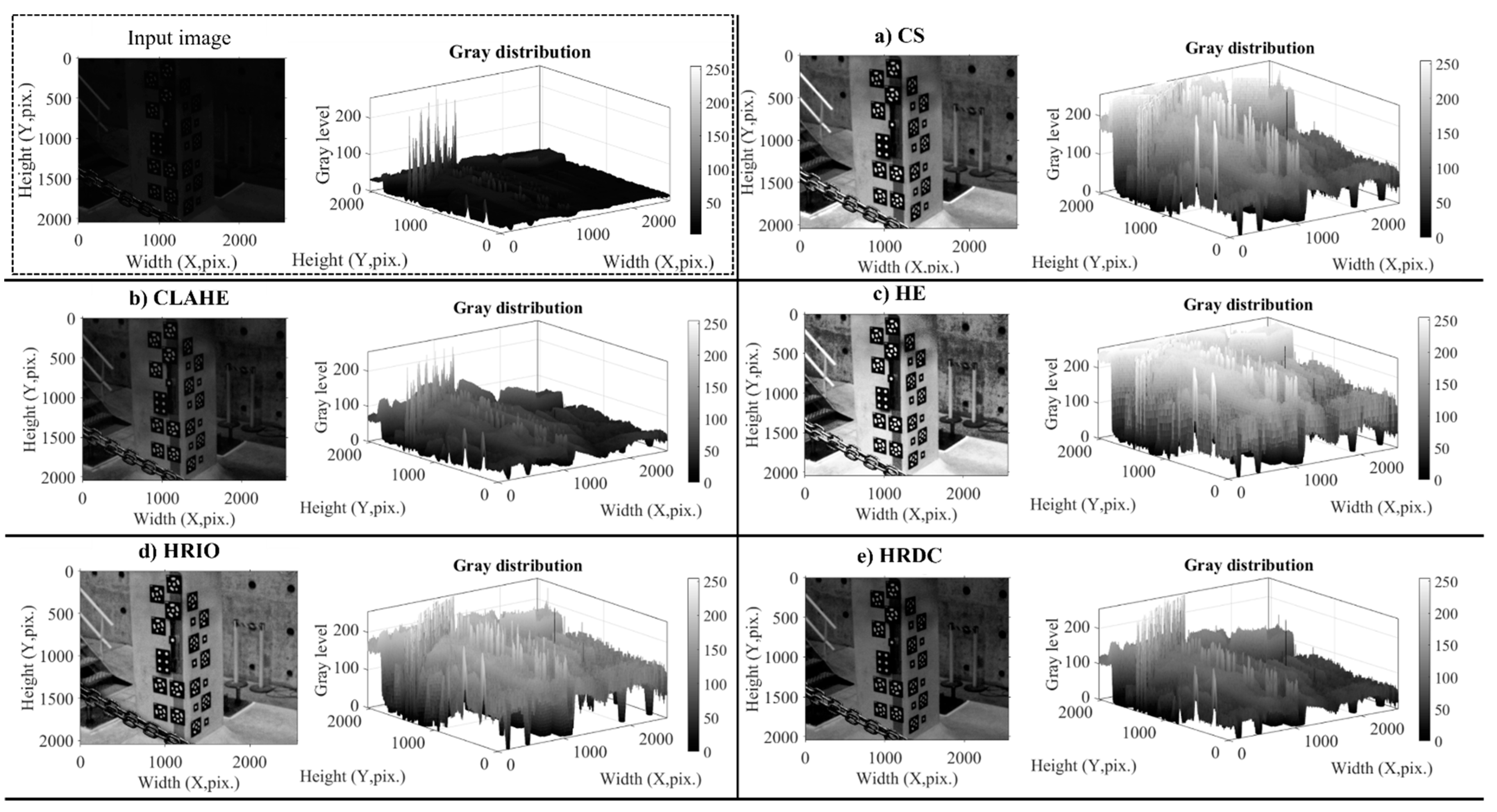
3.2. Output Object Visualization
3.3. Image Quality Assessment
3.4. Effect of Image Enhancement on the Object Identification in the Close-Range Photogrammetry
3.5. Effect of Image Enhancement on the Vision System Measurement Accuracy
4. Implementation in Seismic Monitoring of a Large-Scale Building Using Two Vision-Based Systems
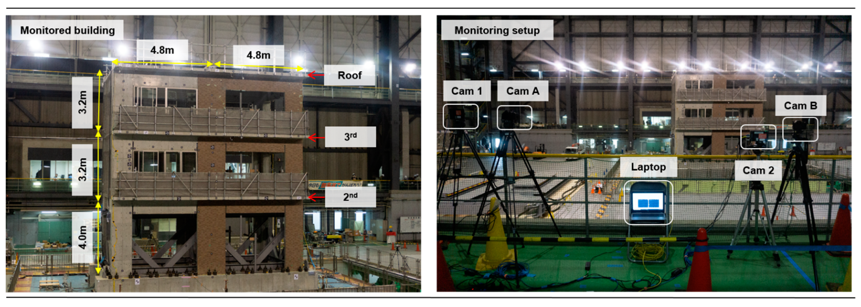
4.1. Monitoring Setup and Building Description
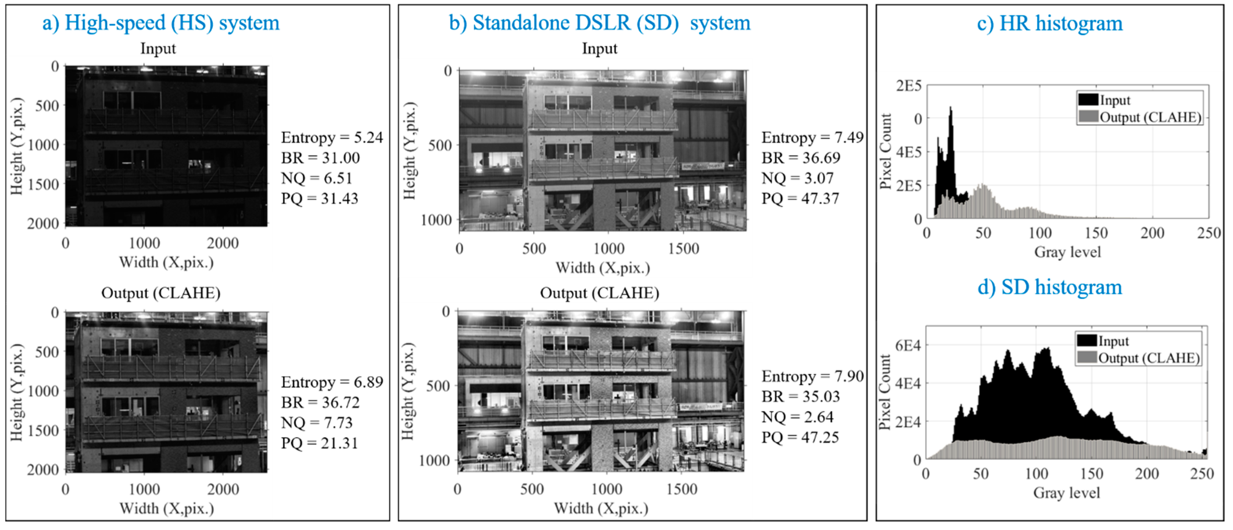
4.2. Output of Image Enhancement
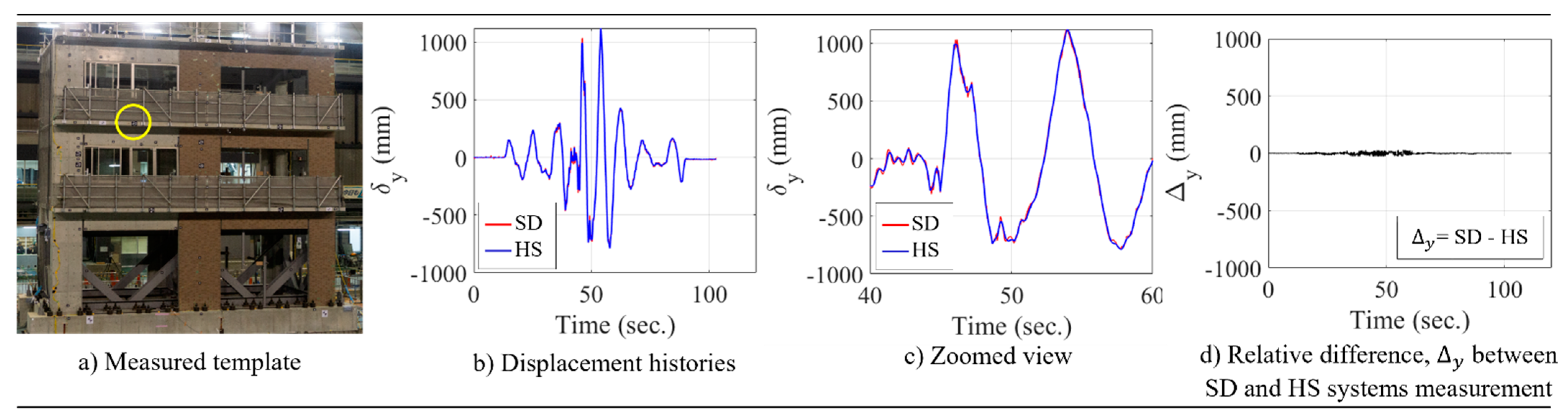
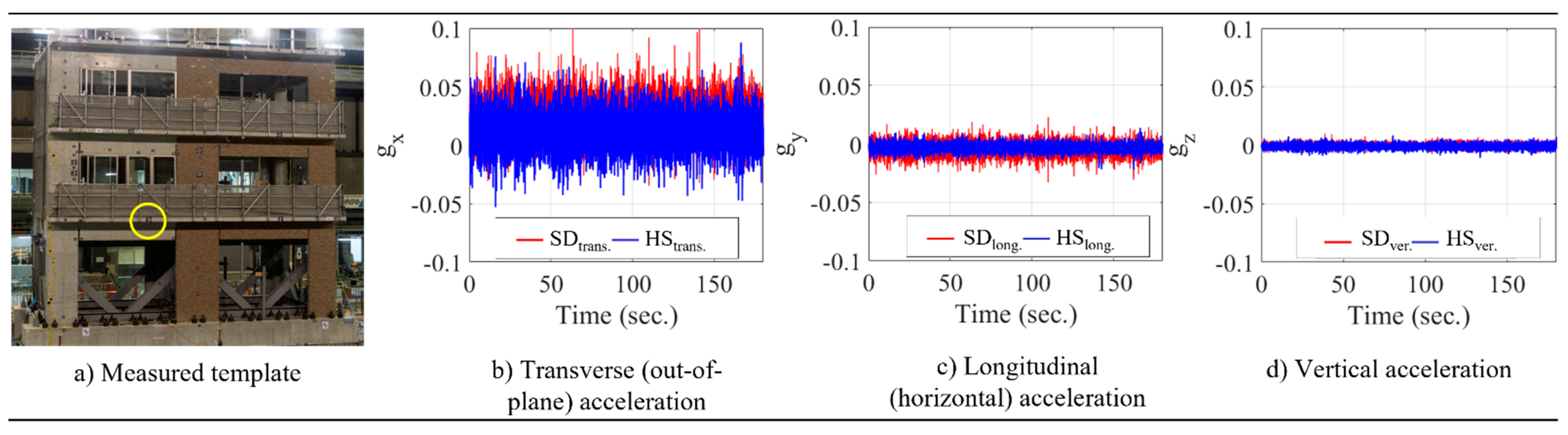
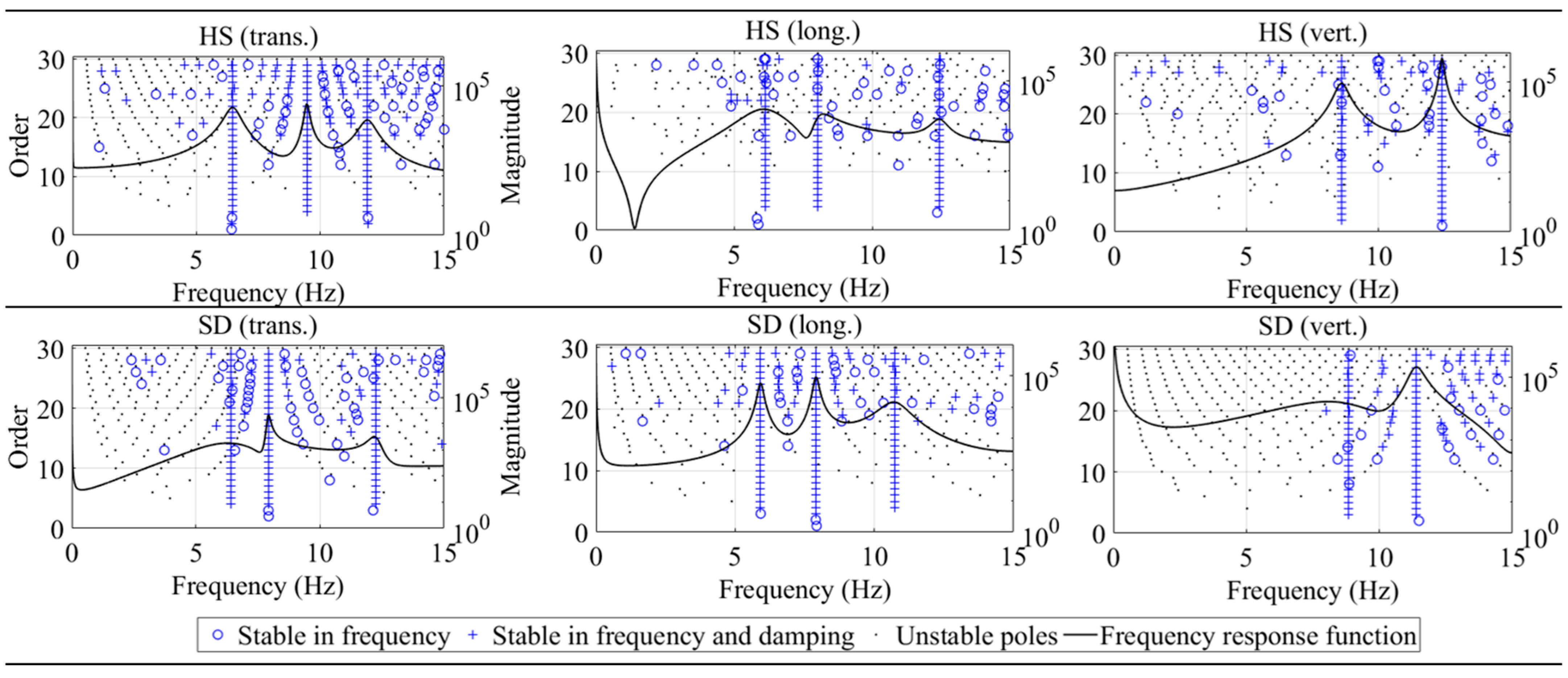
4.3. Seismic Behavior and System Identification of the Three-Story Building
5. Conclusions
- Image enhancement efficiently improves the quality of image data collected from vision-based sensors and needs to be adopted more often in infrastructure and large-scale SHM applications. The proposed algorithms can modify the underexposed and low-contrast input images captured by high-speed or commercial DSLR cameras, thus allowing automatic feature identification. Their efficiency can be estimated through the classical image quality metrics, and their output quality can be assessed by more advanced blind image quality metrics.
- The precision of the enhanced images in measuring static displacement shows a very high accuracy as observed by the two vision systems in the one-inch block test. Comparable results from both systems were also assessed in measuring high-amplitude displacement from the large-scale seismic tests, and in estimating structural modal properties through the system identification procedure.
- Overall, it is concluded that image enhancement does have a significant effect on feature identification and implications for the close-range photogrammetry and SHM accuracy. The applied enhancement algorithms were shown to be computationally effective and are recommended for vision-based SHM image enhancement applications.
- On a specific note, automatic feature detection in enhanced images may be a limitation of this method. Thus, future users are cautioned against selecting the search window and the threshold options for enabling automatic detection of the features on the output images when the global enhancement algorithms are implemented. Instead, a careful check is recommended of the number of obsolete objects identified within each enhanced image plane to allow the bundle adjustment to converge in the photogrammetry process. Measurement accuracy seems to slightly deteriorate when more failed images are identified from the bundle adjustment procedures. With due care, successful monitoring using underexposed and low-contrast images is still possible, not only for different vision system hardware, but also for a wide range of experimental works, through a proper selection of the image enhancement algorithm.
Author Contributions
Funding
Institutional Review Board Statement
Informed Consent Statement
Data Availability Statement
Acknowledgments
Conflicts of Interest
References
- Ngeljaratan, L.; Moustafa, M.A. Structural Health Monitoring and Seismic Response Assessment of Bridge Structures using Target-Tracking Digital Image Correlation. In Engineering Structures; Elsevier: Amsterdam, The Netherlands, 2020; Volume 213, p. 110551. [Google Scholar]
- Ngeljaratan, L.; Moustafa, M.A. System Identification of Large-Scale Bridge Model using Digital Image Correlation from Monochrome and Color Cameras. In Proceedings of the 12th International Workshop on Structural Health Monitoring, Stanford, CA, USA, 10–12 September 2019; DEStech Publications: Pennsylvania, PA, USA, 2019; Volume 2019. [Google Scholar]
- Ngeljaratan, L.; Moustafa, M.A. System Identification of Large-Scale Bridges using Target-Tracking Digital Image Correlation. Front. Built Environ. 2019, 5, 85. [Google Scholar] [CrossRef] [Green Version]
- Ngeljaratan, L.; Moustafa, M.A. Novel Digital Image Correlation Instrumentation for Large-Scale Shake Table Tests. In Proceedings of the 11th NCEE, Los Angeles, CA, USA, 25–29 June 2018; pp. 25–29. [Google Scholar]
- Ngeljaratan, L.; Moustafa, M.A. Digital Image Correlation for Dynamic Shake Table Test Measurement. In Proceedings of the 7th AESE, Pavia, Italy, 6–8 September 2017; pp. 6–8. [Google Scholar]
- Feng, D.; Feng, M.Q. Computer Vision for Structural Dynamics and Health Monitoring; John Wiley & Sons: Hoboken, NJ, USA, 2020. [Google Scholar]
- Feng, D.; Feng, M.Q. Experimental Validation of Cost-Effective Vision-Based Structural Health Monitoring. In Mechanical Systems and Signal Processing; Elsevier: Amsterdam, The Netherlands, 2017; Volume 88, pp. 199–211. [Google Scholar]
- Feng, D.; Feng, M.Q. Vision-based multipoint displacement measurement for structural health monitoring. In Structural Control and Health Monitoring; Wiley Online Library: Hoboken, NJ, USA, 2016; Volume 23, pp. 876–890. [Google Scholar]
- Feng, D. Cable Tension Force Estimate Using Novel Noncontact Vision-Based Sensor. In Measurement; Elsevier: Amsterdam, The Netherlands, 2017; Volume 99, pp. 44–52. [Google Scholar]
- Brownjohn, J.M.W.; Xu, Y.; Hester, D. Vision-Based Bridge Deformation Monitoring. Front. Built Environ. 2017, 3, 23. [Google Scholar] [CrossRef] [Green Version]
- Dong, C.-Z.; Catbas, F.N. A Review of Computer Vision–Based Structural Health Monitoring at Local and Global Levels. In Structural Health Monitoring; SAGE Publications Sage UK: London, UK, 2020. [Google Scholar]
- Ribeiro, D. Non-contact measurement of the dynamic displacement of railway bridges using an advanced video-based system. Eng. Struct. 2014, 75, 164–180. [Google Scholar] [CrossRef]
- Ji, Y.F.; Zhang, O.W. A novel image-based approach for structural displacement measurement. In Proceedings of the Sixth International IABMAS Conference, Lake Maggiore, Italy, 8–12 July 2012; pp. 407–414. [Google Scholar]
- Lee, J.J. Evaluation of bridge load carrying capacity based on dynamic displacement measurement using real-time image processing techniques. Int. J. Steel Struct. 2006, 6, 377–385. [Google Scholar]
- Lee, J.J.; Shinozuka, M. A vision-based system for remote sensing of bridge displacement. Ndt. E Int. 2006, 39, 425–431. [Google Scholar] [CrossRef]
- Olaszek, P. Investigation of the dynamic characteristic of bridge structures using a computer vision method. Measurement 1999, 25, 227–236. [Google Scholar] [CrossRef]
- Ngeljaratan, L.; Moustafa, M.A.; Pekcan, G. A compressive sensing method for processing and improving vision-based target-tracking signals for structural health monitoring. In Computer-Aided Civil and Infrastructure Engineering; Wiley: Hoboken, NJ, USA, 2021; Volume 36, pp. 1203–1223. [Google Scholar]
- Li, J.; Xie, B.; Zhao, X. Measuring the interstory drift of buildings by a smartphone using a feature point matching algorithm. In Structural Control and Health Monitoring; Wiley Online Library: Hoboken, NJ, USA, 2020; Volume 27, p. 2492. [Google Scholar]
- Kim, S.-W. Stay cable tension estimation using a vision-based monitoring system under various weather conditions. J. Civ. Struct. Health Monit. 2017, 7, 343–357. [Google Scholar] [CrossRef]
- Li, J.; Xie, B.; Zhao, X. A Method of Interstory Drift Monitoring Using a Smartphone and a Laser Device. Sensors 2020, 20, 1777. [Google Scholar] [CrossRef] [PubMed] [Green Version]
- Choi, I.; Kim, J.; Jang, J. Development of marker-free night-vision displacement sensor system by using image convex hull optimization. Sensors 2018, 18, 4151. [Google Scholar] [CrossRef] [Green Version]
- Feng, M.Q. Nontarget vision sensor for remote measurement of bridge dynamic response. J. Bridge Eng. 2015, 20, 04015023. [Google Scholar] [CrossRef]
- Yu, Z.; Bajaj, C. A fast and adaptive method for image contrast enhancement. In Proceedings of the 2004 International Conference on Image Processing, Singapore, 24–27 October 2004; Volume 2, pp. 1001–1004. [Google Scholar]
- Thomas, G.; Flores-Tapia, D.; Pistorius, S. Histogram specification: A fast and flexible method to process digital images. IEEE Trans. Instrum. Meas. 2011, 60, 1565–1578. [Google Scholar] [CrossRef]
- Xu, Y. Building crack monitoring based on digital image processing. Frat. Ed Integrità Strutturale 2020, 14, 1–8. [Google Scholar]
- Omar, T.; Nehdi, M.L. Remote sensing of concrete bridge decks using unmanned aerial vehicle infrared thermography. Autom. Constr. 2017, 83, 360–371. [Google Scholar] [CrossRef]
- Russo, F. An image enhancement technique combining sharpening and noise reduction. IEEE Trans. Instrum. Meas. 2002, 51, 824–828. [Google Scholar] [CrossRef]
- Rong, Z.; Jun, W.L. Improved wavelet transform algorithm for single image dehazing. Optik 2014, 125, 3064–3066. [Google Scholar] [CrossRef]
- Abdel-Qader, I.; Abudayyeh, O.; Kelly, M.E. Analysis of edge-detection techniques for crack identification in bridges. J. Comput. Civ. Eng. 2003, 17, 255–263. [Google Scholar] [CrossRef]
- Zhang, R. Automatic Detection of Earthquake-Damaged Buildings by Integrating UAV Oblique Photography and Infrared Thermal Imaging. Remote Sens. 2020, 12, 2621. [Google Scholar] [CrossRef]
- Andreaus, U. Experimental damage evaluation of open and fatigue cracks of multi-cracked beams by using wavelet transform of static response via image analysis. Struct. Control. Health Monit. 2017, 24, e1902. [Google Scholar] [CrossRef]
- Song, Y.-Z. Virtual visual sensors and their application in structural health monitoring. Struct. Health Monit. 2014, 13, 251–264. [Google Scholar] [CrossRef] [Green Version]
- Cha, Y.J. Autonomous structural visual inspection using region-based deep learning for detecting multiple damage types. Comput.-Aided Civ. Infrastruct. Eng. 2018, 33, 731–747. [Google Scholar] [CrossRef]
- Zollini, S. UAV Photogrammetry for Concrete Bridge Inspection Using Object-Based Image Analysis (OBIA). Remote Sens. 2020, 12, 3180. [Google Scholar] [CrossRef]
- Ablin, R.; Sulochana, C.H.; Prabin, G. An investigation in satellite images based on image enhancement techniques. Eur. J. Remote Sens. 2020, 53, 86–94. [Google Scholar] [CrossRef] [Green Version]
- Sidike, P. Adaptive trigonometric transformation function with image contrast and color enhancement: Application to unmanned aerial system imagery. IEEE Geosci. Remote Sens. Lett. 2018, 15, 404–408. [Google Scholar] [CrossRef]
- Brunelli, R. Template Matching Techniques in Computer Vision: Theory and Practice; John Wiley & Sons: Hoboken, NJ, USA, 2009. [Google Scholar]
- Cowan, C.K.; Modayur, B.; DeCurtins, J.L. Automatic Light-Source Placement for Detecting Object Features; International Society for Optics and Photonics: Bellingham, DC, USA, 1992; Volume 1826, pp. 397–408. [Google Scholar]
- Kopparapu, S.K. Lighting design for machine vision application. Image Vis. Comput. 2006, 24, 720–726. [Google Scholar] [CrossRef]
- Luo, L.; Feng, M.Q. Edge-enhanced matching for gradient-based computer vision displacement measurement. Comput.-Aided Civ. Infrastruct. Eng. 2018, 33, 1019–1040. [Google Scholar] [CrossRef]
- Xu, Y.; Brownjohn, J.M.W. Vision-based systems for structural deformation measurement: Case studies. In Proceedings of the Institution of Civil Engineers-Structures and Buildings; Thomas Telford Ltd.: London, UK, 2018; Volume 171, pp. 917–930. [Google Scholar]
- Morgenthal, G.; Hallermann, N. Quality assessment of unmanned aerial vehicle (UAV) based visual inspection of structures. Adv. Struct. Eng. 2014, 17, 289–302. [Google Scholar] [CrossRef]
- Zhu, C. Error estimation of 3D reconstruction in 3D digital image correlation. Meas. Sci. Technol. 2019, 30, 025204. [Google Scholar] [CrossRef]
- Acikgoz, S.; DeJong, M.J.; Soga, K. Sensing dynamic displacements in masonry rail bridges using 2D digital image correlation. Struct. Control. Health Monit. 2018, 25, e2187. [Google Scholar] [CrossRef] [Green Version]
- Poozesh, P. A Multiple Stereo-Vision Approach Using Three Dimensional Digital Image Correlation for Utility-Scale Wind Turbine Blades. In Proceedings of the IMAC XXXVI, Orlando, FL, USA, 12–15 February 2018; SEM: Orlando, FL, USA; Volume 12. [Google Scholar]
- Niezrecki, C.; Baqersad, J.; Sabato, A. Digital image correlation techniques for NDE and SHM. In Handbook of Advanced Non-Destructive Evaluation; Springer: Berlin/Heidelberg, Germany, 2018; pp. 1–46. [Google Scholar]
- Sutton, M.A. Effects of subpixel image restoration on digital correlation error estimates. Opt. Eng. 1988, 27, 271070. [Google Scholar] [CrossRef]
- Wattrisse, B. Analysis of strain localization during tensile tests by digital image correlation. Exp. Mech. 2001, 41, 29–39. [Google Scholar] [CrossRef]
- Bing, P. Performance of sub-pixel registration algorithms in digital image correlation. Meas. Sci. Technol. 2006, 17, 1615. [Google Scholar] [CrossRef]
- Gruen, A. Development and status of image matching in photogrammetry. Photogramm. Rec. 2012, 27, 36–57. [Google Scholar] [CrossRef]
- Bruck, H.A. Digital image correlation using Newton-Raphson method of partial differential correction. Exp. Mech. 1989, 29, 261–267. [Google Scholar] [CrossRef]
- Schreier, H.W.; Braasch, J.R.; Sutton, M.A. Systematic errors in digital image correlation caused by intensity interpolation. Opt. Eng. 2000, 39, 2915–2921. [Google Scholar] [CrossRef]
- Lu, H.; Cary, P.D. Deformation measurements by digital image correlation: Implementation of a second-order displacement gradient. Exp. Mech. 2000, 40, 393–400. [Google Scholar] [CrossRef]
- Zhou, P.; Goodson, K.E. Subpixel displacement and deformation gradient measurement using digital image/speckle correlation. Opt. Eng. 2001, 40, 1613–1621. [Google Scholar] [CrossRef]
- Zhang, J. Application of an improved subpixel registration algorithm on digital speckle correlation measurement. Opt. Laser Technol. 2003, 35, 533–542. [Google Scholar] [CrossRef]
- Luo, L.; Feng, M.Q.; Wu, Z.Y. Robust vision sensor for multi-point displacement monitoring of bridges in the field. Eng. Struct. 2018, 163, 255–266. [Google Scholar] [CrossRef]
- Tian, Y.; Zhang, J.; Yu, S. Vision-based structural scaling factor and flexibility identification through mobile impact testing. Mech. Syst. Signal Process. 2019, 122, 387–402. [Google Scholar] [CrossRef]
- Pilch, A.; Mahajan, A.; Chu, T. Measurement of whole-field surface displacements and strain using a genetic algorithm based intelligent image correlation method. J. Dyn. Syst. Meas. Control 2004, 126, 479–488. [Google Scholar] [CrossRef]
- Jin, H.; Bruck, H.A. Pointwise digital image correlation using genetic algorithms. Exp. Tech. 2005, 29, 36–39. [Google Scholar] [CrossRef]
- Jin, H.; Bruck, H.A. Theoretical development for pointwise digital image correlation. Opt. Eng. 2005, 44, 067003. [Google Scholar] [CrossRef]
- Pitter, M.C.; See, C.W.; Somekh, M.G. Fast Subpixel Digital Image Correlation Using Artificial Neural Networks; IEEE: Piscataway, NJ, USA, 2001; Volume 2, pp. 901–904. [Google Scholar]
- Pitter, M.C.; See, C.W.; Somekh, M.G. Subpixel microscopic deformation analysis using correlation and artificial neural networks. Opt. Express 2001, 8, 322–327. [Google Scholar] [CrossRef] [PubMed]
- Wu, R.-T.; Jahanshahi, M.R. Deep convolutional neural network for structural dynamic response estimation and system identification. J. Eng. Mech. 2019, 145, 04018125. [Google Scholar] [CrossRef]
- Zhang, Y. Autonomous bolt loosening detection using deep learning. Struct. Health Monit. 2020, 19, 105–122. [Google Scholar] [CrossRef]
- Chen, S. UAV bridge inspection through evaluated 3D reconstructions. J. Bridge Eng. 2019, 24, 05019001. [Google Scholar] [CrossRef] [Green Version]
- Yin, Z.; Wu, C.; Chen, G. Concrete crack detection through full-field displacement and curvature measurements by visual mark tracking: A proof-of-concept study. Struct. Health Monit. 2014, 13, 205–218. [Google Scholar] [CrossRef]
- Schneider, C.T. 3-D Vermessung von Oberflächen und Bauteilen durch Photogrammetrie und Bildverarbeitung. Proc. IDENT/VISION 1991, 91, 14–17. [Google Scholar]
- Lindeberg, T. Feature detection with automatic scale selection. Int. J. Comput. Vis. 1998, 30, 79–116. [Google Scholar] [CrossRef]
- Lindeberg, T. Edge detection and ridge detection with automatic scale selection. Int. J. Comput. Vis. 1998, 30, 117–156. [Google Scholar] [CrossRef]
- Pathak, S.S.; Dahiwale, P.; Padole, G. A Combined Effect of Local and Global Method for Contrast Image Enhancement; IEEE: Piscataway, NJ, USA, 2015; pp. 1–5. [Google Scholar]
- Jain, A.K. Fundamentals of Digital Image Processing; Prentice-Hall: Hoboken, NJ, USA, 1989. [Google Scholar]
- Lidong, H. Combination of contrast limited adaptive histogram equalisation and discrete wavelet transform for image enhancement. IET Image Process. 2015, 9, 908–915. [Google Scholar] [CrossRef]
- Dong, X. Fast Efficient Algorithm for Enhancement of Low Lighting Video; IEEE: Piscataway, NJ, USA, 2011; pp. 1–6. [Google Scholar]
- He, K.; Sun, J.; Tang, X. Single image haze removal using dark channel prior. IEEE Trans. Pattern Anal. Mach. Intell. 2010, 33, 2341–2353. [Google Scholar] [PubMed]
- Mittal, A.; Moorthy, A.K.; Bovik, A.C. Blind/Referenceless Image Spatial Quality Evaluator; IEEE: Piscataway, NJ, USA, 2011; pp. 723–727. [Google Scholar]
- Mittal, A.; Soundararajan, R.; Bovik, A.C. Making a “completely blind” image quality analyzer. IEEE Signal Process. Lett. 2012, 20, 209–212. [Google Scholar] [CrossRef]
- Venkatanath, N. Blind Image Quality Evaluation Using Perception Based Features; IEEE: Piscataway, NJ, USA, 2015; pp. 1–6. [Google Scholar]
- Stephen, G.A.; Brownjohn, J.M.W.; Taylor, C.A. Measurements of static and dynamic displacement from visual monitoring of the Humber Bridge. Eng. Struct. 1993, 15, 197–208. [Google Scholar] [CrossRef] [Green Version]
- Yeow, T.Z.; Kusunoki, K.; Nakamura, I.; Hibino, Y.; Fukai, S.; Safi, W.A. E-Defense Shake-table Test of a Building Designed for Post-disaster Functionality. J. Earthq. Eng. 2021, 2, 1–22. [Google Scholar] [CrossRef]


| Camera Type | High-Speed (HS) | Standalone DSLR (SD) |
|---|---|---|
| Standalone | No | Yes |
| Sensor | CMOS | CMOS |
| Color | Monochrome | Monochrome |
| Depth, | 8 | 8 |
| Input image size, (pixel) | 2560 2048 | 5184 2912 |
| f-stop number | ||
| Shutter speed | ||
| File type | .tiff | .jpg |
| Point | 1 | 2 | 3 | 4 | 5 | 6 | 1 | 2 | 3 | 4 | 5 | 6 | ||
|---|---|---|---|---|---|---|---|---|---|---|---|---|---|---|
| CS (a) | 19.09 | 19.18 | 18.75 | 19.3 | 19.32 | 19.38 | 2.41 | 15.95 | 15.91 | 15.19 | 16.24 | 16.41 | 16.31 | 5.56 |
| CLAHE (b) | 19.81 | 19.73 | 19.69 | 20.33 | 20.46 | 20.28 | 3.42 | 16.59 | 16.2 | 17.17 | 17.4 | 17.4 | 17.19 | 5.75 |
| HE (c) | 20.89 | 21 | 20.7 | 20.97 | 20.94 | 20.99 | 1.08 | 17.65 | 17.57 | 17.01 | 17.71 | 17.78 | 17.63 | 3.17 |
| HRIO (d) | 19.1 | 18.55 | 18.58 | 20.39 | 20.68 | 20.96 | 11.08 | 16.1 | 15.41 | 15.2 | 17.26 | 17.62 | 17.88 | 14.00 |
| HRDC (e) | 20.73 | 20.98 | 20.66 | 20.85 | 21.07 | 20.93 | 1.48 | 17.44 | 17.51 | 17.02 | 17.59 | 17.8 | 17.61 | 3.00 |
| 4.33 | 5.48 | 5.13 | 3.24 | 3.40 | 3.40 | 4.60 | 5.89 | 6.29 | 3.39 | 3.32 | 3.57 | |||
| Method | Index | Method | Index | ||||||||
|---|---|---|---|---|---|---|---|---|---|---|---|
| CS | 2.74 | 8.08 | 11.01 | 1.78 | 5.04 (b) | 5.19 (a) | CS | 0.96 | 4.96 | 12.66 | 89.31 |
| CLAHE | 0.86 (b) | 2.62 (b) | 4.43 (b) | 1.96 | 6.02 | 4.46 | CLAHE | 23.46 | 12.43 (a) | 8.90 (b) | 17.04 (b) |
| HE | 2.71 | 2.75 | 14.90 | 2.07 | 5.93 | 4.45 | HE | 0.19 (b) | 4.72 (b) | 10.40 | 87.04 |
| HRIO | 1.61 | 5.73 | 7.44 | 1.65 (b) | 6.61 | 1.74 (b) | HRIO | 37.88 (a) | 6.37 | 10.78 | 103.62 (a) |
| HRDC | 6.10 (a) | 15.36 (a) | 15.18 (a) | 5.25 (a) | 9.41 (a) | 3.35 | HRDC | 22.31 | 5.75 | 14.16 (a) | 83.58 |
| Method | Total | Correct | % | Incorrect | % | Non-Object | % | Unidentified | % | Failed Images (Out of 50) |
|---|---|---|---|---|---|---|---|---|---|---|
| CS | 1963 | 1233 | 62.81 | 668 | 34.03 | 68 | 3.46 | −6 | −0.30 | 0 |
| CLAHE | 1897 | 1215 | 64.05 | 636 | 33.53 | 49 | 2.58 | −3 | −0.16 | 0 |
| HE | 2040 | 1278 | 62.65 | 678 | 33.24 | 85 | 4.17 | −1 | −0.05 | 0 |
| HRIO | 1466 | 1174 | 80.08 | 201 | 13.71 | 91 | 6.21 | 0 | 0 | 1 |
| HRDC | 1178 | 965 | 81.92 | 178 | 15.11 | 35 | 2.97 | 0 | 0 | 10 |
| Method | (pix.) | (pix.) | (pix.) |
|---|---|---|---|
| CS | 7135.09 | −35.01 | −7.06 |
| CLAHE | 7154.47 | −24.22 | −8.28 |
| HE | 7156.03 | −28.39 | −9.81 |
| HRIO | 7181.46 | −31.85 | −12.01 |
| HRDC | 7160.54 | −38.92 | −12.95 |
| (%) | 0.23 | −18.00 | −24.64 |
| Measurement | Point | Measurement | Point | ||||||||||||
|---|---|---|---|---|---|---|---|---|---|---|---|---|---|---|---|
| 1 | 2 | 3 | 4 | 5 | 6 | 1 | 2 | 3 | 4 | 5 | 6 | ||||
| (1) | (mm) | 25.83 | 24.92 | 25.35 | 25.47 | 25.79 | 25.32 | (4) | (mm) | 24.70 | 24.96 | 25.18 | 25.40 | 25.48 | 25.43 |
| (%) | 1.71 | 1.89 | 0.18 | 0.27 | 1.55 | 0.31 | (%) | 2.76 | 1.75 | 0.85 | 0.01 | 0.30 | 0.14 | ||
| (%) | 0.98 | (%) | 0.97 | ||||||||||||
| (2) | (mm) | 24.95 | 25.02 | 25.20 | 25.56 | 25.59 | 25.41 | (5) | (mm) | 25.81 | 24.91 | 25.14 | 25.65 | 25.82 | 25.14 |
| (%) | 1.79 | 1.50 | 0.78 | 0.65 | 0.74 | 0.06 | (%) | 1.63 | 1.94 | 1.02 | 1.00 | 1.64 | 1.01 | ||
| (%) | 0.92 | (%) | 1.37 | ||||||||||||
| (3) | (mm) | 24.83 | 25.01 | 25.20 | 25.44 | 25.58 | 25.51 | (6) | (mm) | 25.06 | 25.03 | 25.14 | 25.22 | 25.15 | 25.51 |
| (%) | 2.26 | 1.53 | 0.78 | 0.18 | 0.71 | 0.45 | (%) | 1.34 | 1.46 | 1.02 | 0.71 | 0.98 | 0.43 | ||
| (%) | 0.98 | (%) | 0.99 | ||||||||||||
| Type | High-Speed (HS) | Standalone DSLR (SD) |
|---|---|---|
| Color | Monochrome | Monochrome |
| Format | .tiff | .jpg |
| Input image size (pixel) | 2560 2048 | 1920 1080 |
| Sampling rates, (frame-per-second) | 32 | 30 |
| Seismic record duration (s) | 120 | 120 |
| White noise record duration (s) | 180 | 180 |
| System | (mm) | (mm) | System | (mm) | (mm) | ||
|---|---|---|---|---|---|---|---|
| (mm) | (%) | ||||||
| HS | 1118.3 | −787.4 | SD | 1113.3 | −779.2 | −28.57 | 3.63 |
| Transverse Mode | |||||||||
| System | (Hz) | System | (Hz) | (%) | System | (%) | System | (%) | (%) |
| HS | 6.47 | SD | 6.44 | 0.46 | HS | 4.65 | SD | 4.51 | 3.01 |
| Longitudinal Mode | |||||||||
| System | (Hz) | System | (Hz) | (%) | System | (%) | System | (%) | (%) |
| HS | 6.12 | SD | 5.91 | 3.43 | HS | 2.53 | SD | 2.61 | 3.16 |
| Vertical Mode | |||||||||
| System | (Hz) | System | (Hz) | (%) | System | (%) | System | (%) | (%) |
| HS | 8.59 | SD | 8.84 | 2.91 | HS | 2.70 | SD | 2.62 | 2.96 |
Publisher’s Note: MDPI stays neutral with regard to jurisdictional claims in published maps and institutional affiliations. |
© 2021 by the authors. Licensee MDPI, Basel, Switzerland. This article is an open access article distributed under the terms and conditions of the Creative Commons Attribution (CC BY) license (https://creativecommons.org/licenses/by/4.0/).
Share and Cite
Ngeljaratan, L.; Moustafa, M.A. Underexposed Vision-Based Sensors’ Image Enhancement for Feature Identification in Close-Range Photogrammetry and Structural Health Monitoring. Appl. Sci. 2021, 11, 11086. https://doi.org/10.3390/app112311086
Ngeljaratan L, Moustafa MA. Underexposed Vision-Based Sensors’ Image Enhancement for Feature Identification in Close-Range Photogrammetry and Structural Health Monitoring. Applied Sciences. 2021; 11(23):11086. https://doi.org/10.3390/app112311086
Chicago/Turabian StyleNgeljaratan, Luna, and Mohamed A. Moustafa. 2021. "Underexposed Vision-Based Sensors’ Image Enhancement for Feature Identification in Close-Range Photogrammetry and Structural Health Monitoring" Applied Sciences 11, no. 23: 11086. https://doi.org/10.3390/app112311086
APA StyleNgeljaratan, L., & Moustafa, M. A. (2021). Underexposed Vision-Based Sensors’ Image Enhancement for Feature Identification in Close-Range Photogrammetry and Structural Health Monitoring. Applied Sciences, 11(23), 11086. https://doi.org/10.3390/app112311086