Leveraging Expert Knowledge for Label Noise Mitigation in Machine Learning

Abstract

In training-based Machine Learning applications, the training data are frequently labeled by non-experts and expose substantial label noise which greatly alters the training models. In this work, a novel method for reducing the effect of label noise is introduced. The rules are created from expert knowledge to identify the incorrect non-expert training data. Using the gradient descent algorithm, the violating data samples are weighted less to mitigate their effects during model training. The proposed method is applied to the image classification problem using Manga109 and CIFAR-10 dataset. The experiments show that when the noise level is up to 50% our proposed method significantly increases the accuracy of the model compared to conventional learning methods.

1. Introduction

Machine learning algorithms have been extensively applied in various fields and achieved substantial success. However, there are various issues when machine learning is operated in real-world applications as many practical issues arise. The label noise issue is one of the problems that drastically reduces the supervised machine learning algorithms’ accuracy [1,2].

Label noise appears when the label for training is incorrectly assigned to instances in the training set. This often occurs due to the use of non-experts for labeling, especially when labels are made with crowd-sourcing methods [3]. It is difficult to completely prevent label noise because labeling is performed by humans and the data set required for machine learning is very large. It is very expensive to sort label noise from such a huge amount of data manually. Therefore, label noise can be considered the biggest challenge in supervised machine learning [4].

1.1. Related Works

Some considerable solutions have been proposed to overcome the label noise problem. The solutions can be categorized into three main approaches. The first approach relies on the fact that some algorithms are more robust to noise data than the others. In many works, by adjusting the training processes and loss functions, the models themselves are modified for improving robustness to label noise. For example, a smooth loss like hinge loss, squared loss, exponential loss, and log-loss can be easily affected by label noise than hard loss [5,6]. Ref. [7] has modified the training procedure of neural networks to reduce the effect of label noise. Refs. [8,9] use ensemble methods like boosting to make the model more robust with label noise; and Dietterich [10] concludes that boosting is less effective than bagging to deal with this problem. Refs. [11,12] detect label noise based on their change of the classification of other samples in a leave-one-out framework. Furthermore, probabilistic models with a novel form have been used and also improve the performance of the classifier [13,14].

The second approach is called “filter framework” and the algorithms consist of two separated parts. First, the label noise detection detects the label noise in the training dataset. Second, the label noise processing part uses a technique to mitigate the label noise effect. The most beneficial advantage of this framework is that it facilitates to create new algorithms that combine the strength of each part. Outlier detection based algorithms detect if the label noise sample is corresponding to an outlier sample, whose anomaly score exceeds a predefined threshold [15,16]. Many algorithms use a model that trained from the original training set to classify the training set itself to detect the label noise [17,18]. This method might suffer from the egg–chicken dilemma, as the model is trained using the training set with label noise and it may lead to bad performance, causing bad prediction of label noise as well as bad overall performance. To avoid this problem, the ensembles method is used to detect label noise more precisely [19,20]. K-fold cross-validation is used to group K different pairs of training and validation sets, and each pair is used to train m different models using m different algorithms. After that, each instance in the corresponding validation set is classified by m models to detect the label noise. After label noise is detected, the simplest solution is to remove it from the training set, and retrain the model from the data set with label noise removed. However, this may lead to removing a lot of data resulting in bad training performance. A more complex algorithm is to weight the samples in the training set, which comes from the fact that the effect of each sample on the model can be different. Refs. [21,22] down-weight the data samples that are likely label noise and train the model from the weighted data set.

The third approach exploits expert knowledge and put it into the learning process. Ref. [23] converts knowledge into first-order logic (FOL) as constraints and then optimizes loss function subjected to those conditions. The deep-learning network in [23] is modified for integrating the FOL into the system. Although the performance of the modified deep-learning algorithm is good, it requires the change of the network structure which may cause difficulty in practical implementation.

1.2. Contributions

In this work, to deal with Noise Not At Random (NNAR), we propose a new method derived from the filter framework with the expert knowledge being used in the label noise detection part. By incorporating the advantages of the second and third approaches, not only expert knowledge about the training dataset is exploited, but the method can also be combined with other algorithms for label noise processing part to maximize the effect of removing label noise. In detail, our method leverages expert knowledge about the training dataset to detect label noise samples in the label-noise-detection part of the filter framework. Unlike the previous works, the proposed method is applicable for every learning algorithm, and does not require any change in the main model structure, thereby shortening the project implementation time and cost. For evaluating our algorithm, conventional training algorithm, and two other related works are used in the image classification problem on Manga109 [24,25] and CIFAR-10 [26] dataset. The experimental results show that, when level of label noise is high, our method achieves higher accuracy than the related works and conventional learning.

Our contributions are summarized as follows:

• We have established a new method that leverages the experts’ knowledge for enhancing the learning model in the presence of label noise without changing the model structure. The proposed method is simple, intuitive, explainable, applicable for every learning algorithm, and can combine with other algorithms.
• The proposed method is realized as two algorithms: “Rule-Weight” algorithm weights the data sample differently to partially alleviate the bad effect in the sample; “Rule-Remove” algorithm excludes the bad sample from the training model. The performance comparison with the algorithms in [27] show that the Rule-Weight is the best even when the level of label noise in the dataset is as high as 50%.
• The experiments on image processing problem confirm that the label noise can be detected by simple pre-defined rules created from the expert knowledge.

1.3. Organization

The rest of the manuscript is organized as follows. In Section 2, the proposed methodology is introduced. Section 3 describes the dataset, the implementation of algorithm in this dataset and experimental setup. The simulation results are described and analyzed in Section 4 and Section 5 conclude the work.

2. Materials & Methods

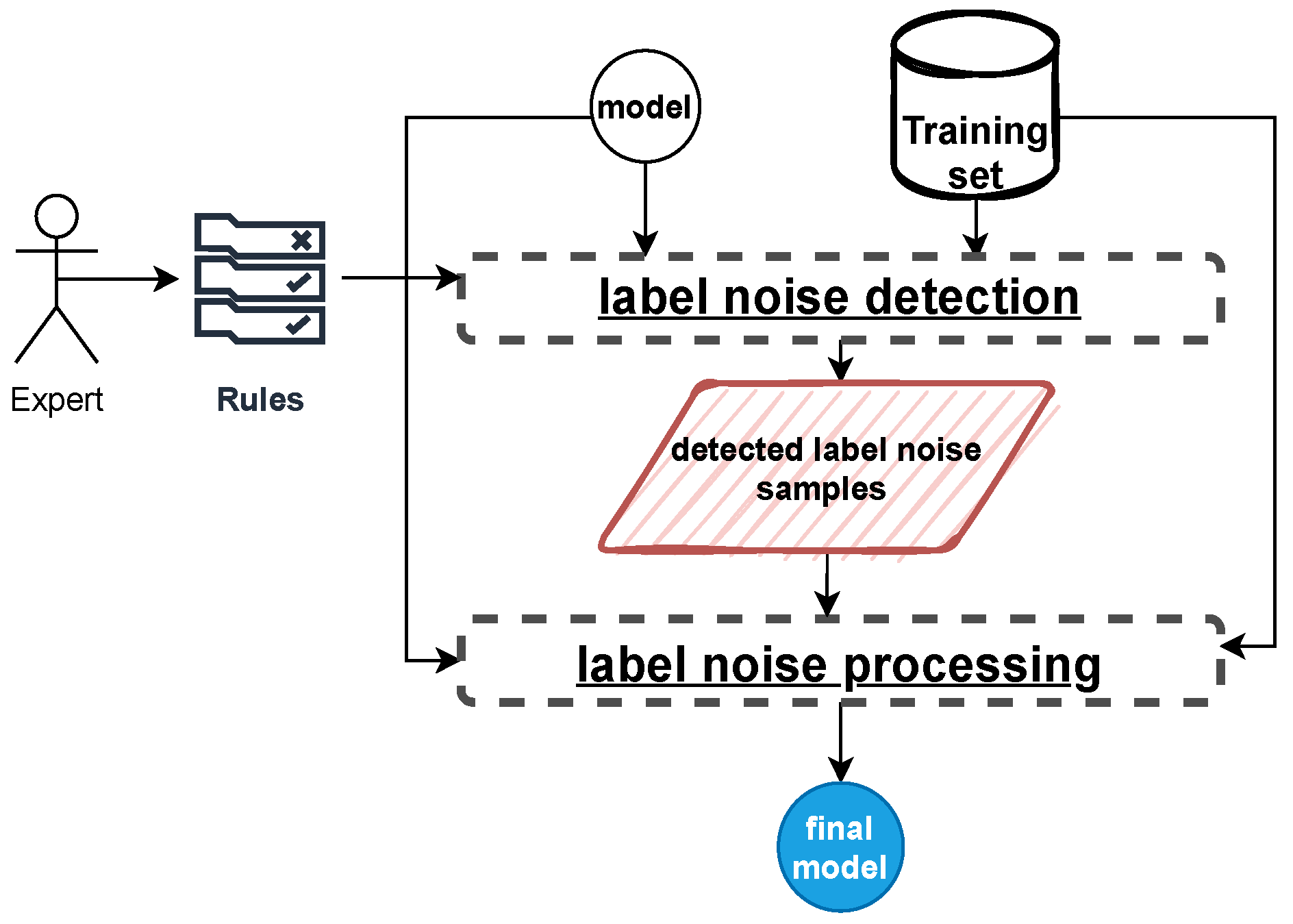
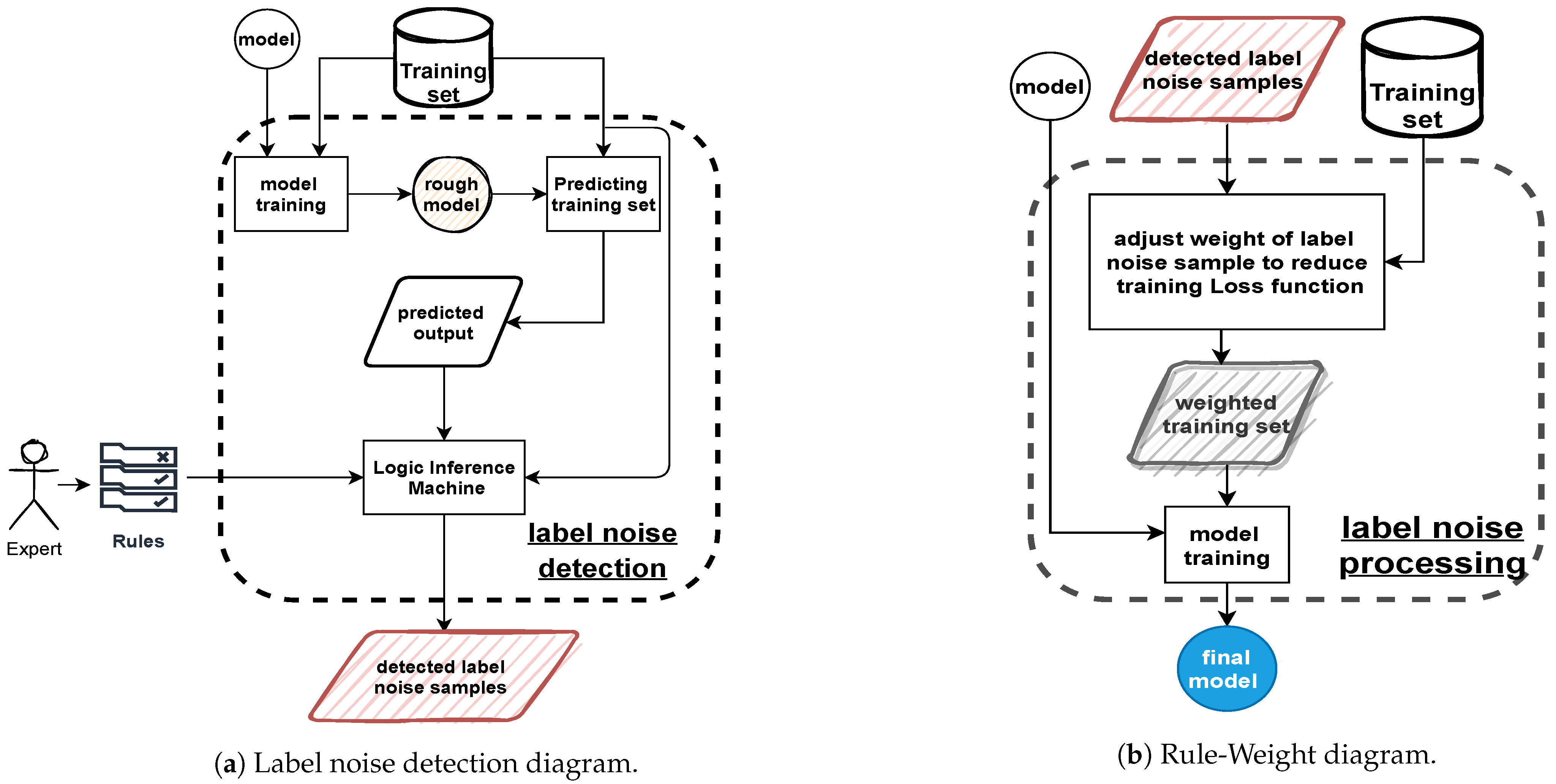
2.1. Methodology Overview

We propose a methodology derived from the filter framework consisting of label noise detection part and label noise processing part, as shown in Figure 1. Unlike the aforementioned traditional approaches, where only training data are used to train the model, rules created by experts are added to this framework to first detect the label noise samples. The label noise detector utilizes the rules, the non-expert training set, and the learning model created by the training set. The detected data samples are used as input of the label noise processor to train a better model than when the only non-expert training set is available.

The detail of the proposed label noise detector is shown in Figure 2a. First, a machine learning model is trained from the non-expert training data, and then that model is used to predict the non-expert training data. An assumption here is that this model still has good enough performance, despite suffering from the label noise. The main reason people wrongly assign labels is that data samples are quite similar to other data in the different class. Consequently, these label noise samples are misclassified with high probability. Hence, based on the rules derived from expert knowledge, a Logic Inference Machine detects a set of data with a predicted output that violates the rules and differs from the label. Most of the label noise is included in this set, and this set is considered the detected label noise set. Unlike traditional methods [28,29], the rules derived from expert knowledge are added to detect the label noise more precisely. A data sample is considered as label noise not only its predicted output differs from the label, but also violates the rules. This reduces the number of normal data samples that are wrongly detected as label noise.

The label noise processing part can be any algorithms to treat with detected label noise to train a better model. Consequently, the output model suffers less from label noise, and the effect of label noise in the output training set is mitigated.

Based on that method, two algorithms are proposed: Rule-Remove and Rule-Weight. The label noise processing part of Rule-Remove completely remove the detected label noise data samples, and train the model from the removed label noise data set. On the other hand, the label noise processing part of Rule-Weight weight the detected label noise data samples, and train the model from the weighted data set. Rule-Remove algorithm can be considered as a special case of Rule-Weight when weight is set to zero at the detected label noise samples. Therefore, only the Rule-Weight algorithm is described in detail in this section.

2.2. Rule-Weight Algorithm

The label noise processing part of the Rule-Weight algorithm is shown in Figure 2b. First, the detected label noise samples are weighted to reduce the bad influence of the data to the model training. Then the model is retrained with weighted data. As such, the loss function for model training is less affected by label noise data samples. Therefore, the model is more accurate.

Algorithm 1 shows the procedure for updating the weight, and training the model in Rule-Weight algorithm. To speed up the training process, the training set is split into smaller mini-batches and the loss function is calculated for each mini-batch. The update process is executed for each mini-batch data sample and stops after a predefined number of loops T. First of all, a $roughModel$ is trained from an initial model $model$ using the training algorithm $trainAlgo\left(\right)$ with whole training set $TrainingSet$. Let $j(Y,Label)$ be the distance between the label $Label$ of all samples in $TrainingSet$ and its predicted output Y and $ϵ$ is the weight vector for each data sample in $TrainingSet$, the loss function is defined as $\overline{L}(ϵ\odot j(Y,Label))$, where ⊙ is the element-wise dot product. At the beginning, all elements of $ϵ$ are 1, i.e., all the data samples are treated equally. The model is trained according to weighted data samples at every step. Therefore, a temporary variable $Mode{l}_t$ is declared to store the temporary model at every step t and at initialization step $Mode{l}_0$ is assigned to $model$. At loop t, a mini-batch data sample $X_t$ and the corresponding label $Labe{l}_t$ is randomly drawn from training set by the function $SampleMiniBatch\left(\right)$. After that, the $roughModel$ is used to predict the output $Y_t$ of the mini-batch data sample $X_t$. The logical inference machine $RuleCheck\left(\right)$ checks if the predicted output $Y_t$ of the input $X_t$ violates the given rules and differs from the label $Labe{l}_t$. In other words, a data sample is considered as a correct label if its predicted output is equal to its label or the relationships between that data sample and its predicted output satisfy all given rules. The violating data samples are put in the label noise set $D_t$. Most of the label noise are in $D_t$ and should be weighted less than the non-violating data to reduce their effect. The optimal weight can be found by applying the gradient descent algorithm for the mini-batch data. This optimal weight is used to train the temporary model $Mode{l}_t$ later. To do that, the loss of model $Mode{l}_t$ for the $j^{th}$ data sample of $D_t$ is calculated using $Los{s}_j\left(\right)$. The gradient $g_t$ is calculated over all data samples in the set $D_t$ using the calculated loss. The weight ${ϵ}_{t+1}$ for each data sample in $X_t$ is updated based on the gradient $g_t$ with learning rate $\alpha$. Initially, all elements of ${ϵ}_0$ are 1. After obtaining the proper weight, a weighted mini-batch data $WeightedM{B}_t$ is formed by updating these weights for $X_t$ at $Weight\left(\right)$ function. $WeightedMB$ = [${ϵ}_{t+1}$,$X_t$,$Labe{l}_t$]. $WeightedMB$ is then used to train $Mode{l}_t$ which should be more accurate than the previous one. The loss function in the training algorithm $trainAlgo\left(\right)$ is $\overline{L_t}({ϵ}_{t+1}\odot j(Y_t,Labe{l}_t))$. The $FinalModel$ is the $Mode{l}_t$ after T times training with the weighted mini-batch data sample.

Algorithm 1 Rule-Weight.

Require:TrainingSet, trainAlgo(),model, α, T

Ensure:FinalModel

roughModel ⇐ trainAlgo(model, TrainingSet)

Model0 ⇐ model

for t = 0 to T do

Xt, Labelt ⇐ SampleMiniBatch(TrainingSet)

Yt ⇐ roughModel(Xt)

Dt ⇐ RuleCheck(Xt, Yt, Labelt)

gt ⇐ $\frac{ə}{ə{ϵ}_t}\frac{1}{\left|D_t\right|}{\sum }_{j∊D_t}$ Lossj(Modelt, Yt, Labelt)

ϵt+1 ⇐ max(ϵt − α.gt, 0)

WeightedMBt ⇐ Weight(Xt, Labelt, Dt, ϵt+1)

Modelt+1 ⇐ trainAlgo(Modelt,WeightedMBt)

end for

FinalModel ⇐ ModelT

2.3. Rule-Remove Algorithm

Algorithm 2 shows the pseudo code of the Rule-Remove algorithm. In general, it is similar to the Rule-Weight algorithm, except that the violating data are removed instead of weighted. In other words, the Rule-Remove algorithm is the Rule-Weight algorithm with the violating data samples being weighted zeros. In detail, after detecting the label noise set $D_t$, a mini-batch data $WeightedMB$ is formed by removing $D_t$ from $X_t$. In other words, the coefficient of the violating data samples in $D_t$ are set to zero in $X_t$. After that, $WeightedMB$ is used to train $Mode{l}_t$. Unlike the traditional approach, if the $roughModel$ is not well trained, a lot of data samples are removed, leading to bad performance of $FinalModel$. However, the proposed algorithm is able to avoid this problem because a data sample is considered to be label noise not only when its predicted output $Y_t$ differs from the label $Labe{l}_t$ but also when $Y_t$ violates the given rules. Thanks to the removal of the violating data samples, the running time of the Rule-Remove algorithm is faster than the Rule-Weight algorithm. Both algorithms are evaluated in Section 3.

Algorithm 2 Rule-Remove.

Require:TrainingSet, trainAlgo(),model, T

Ensure:FinalModel

roughModel ⇐ trainAlgo(model, TrainingSet)

Model0 ⇐ model

for t = 0 to T do

Xt, Labelt ⇐ SampleMiniBatch(TrainingSet)

Yt ⇐ roughModel(Xt)

Dt ⇐ RuleCheck(Xt, Yt, Labelt)

WeightedMBt ⇐ Weight(Xt, Labelt, Dt, ϵt+1 = 0)

Modelt+1 ⇐ trainAlgo(Modelt,WeightedMBt)

end for

FinalModel ⇐ ModelT

3. Experiments

This experiment uses Manga109 dataset [24,25] and CIFAR-10 dataset [26] to appraise the performance of two proposed algorithms. In experiments, label noise is artificially generated in the training data, and the accuracy for the test set of the model constructed by the proposed method is measured. Label noise is generated so that it represents labeling mistakes that are likely to be caused by humans. As such, the label noise is created based on the classification model Confusion Matrix, which is trained based on training data that do not contain noise. In the C-classes classification problem, the confusion matrix is a $C\times C$ matrix that summarizes the results. The ith row shows how the cases of the ith class were classified. First, the correct original dataset is used to train a model. Then, the trained model is used to the classify that original dataset and this prediction is the noisy label.

To evaluate the effect of the proposed method, the experiments are performed with six algorithms as follows:

• Normal learning algorithm. The classification model is performed without removing label noise.
• Classification Filtering [29] (CF) is an algorithm on filter framework which use a model that trained from the original noisy training set to classify the training set itself, and remove samples that its predicted output differs from its label
• LC-True algorithm [27].
• LC-Est algorithm [27].
• Rule-Remove algorithm.
• Rule-Weight (RW) algorithm.

The third and fourth algorithms are derived from the Loss Correction Approach [27]. In their approach, loss function is changed based on the noise transition matrix T to make the model robust with label noise. The noise transition matrix T is the matrix whose element $T_{ij}$ in row ith column jth present the probability of a data sample from classes i is incorrectly labeled to class j. [27] proposed two approaches to refine loss function during training in the noisy data: forward and backward. In the forward case, the refined prediction is normal prediction multiply with T and in the backward case, multiplying $T^{-1}$ with loss during back-propagation give the refined loss. Only LossCorrection forward is compared in this article since it work better than backward, and it is denoted by LossCorrection for short. The LC-True algorithm ideally assumes that the T matrix is well-known while LC-Est algorithm has to estimate it. Here, the LC-True is used as a benchmark algorithm because it is very rare for the T matrix to be known in advance in practice.

3.1. Experiment on Manga109

In Manga109, the main task is to predict the author name from the image of the face of each manga character.

3.1.1. Dataset

Manga109 [24,25] is the largest dataset for Japanese comics (manga), consisting of 109 volumes drawn by 92 professional Japanese manga artists. Each volume has many attributes such as the name of author, publisher, target’s readership, genre, page numbers, and the target age, which are useful for the logical reasoning mechanism to handle. This is the reason that this dataset is chosen to evaluate our algorithms.

Figure 3a shows an example of the annotation in the Manga109 dataset. The information of each volume is included in the corresponding XML file, including many fields such as ID and name of each character present in that volume and the information of each object in each page in that volume. Face, body, text, and frame are the four types of objects annotated in each page, determined by coordinates of the four points that form a rectangle surrounding the object. Not only that, face and body are also determined by character id, text fields also include text content. Figure 3b illustrates an image with the red, blue, yellow, and green rectangle surround the face, body, text, and frame.

The object images in Manga109 dataset have diverse sizes and could be gray or color images depending on each volume. As the average of both vertical and horizontal sizes in all the images is 24, therefore, in this study, the size of all images is converted to $24\times 24$ pixels and gray-scale the color image. The input of this classification task is the character’s face images and the output is the author’s name. One data sample corresponds to a $24\times 24\times 1$ face image and we assume that the publisher, target’s readership, and genre of the volume that contain that image is the prior knowledge about that image, and it is used to make a logic inference, but not be used in the classification process. The label of a data sample is the name of the author that draws the image.

There are 92 classes and the distribution of number of samples each class is shown in Figure 4. There are 8 outlier classes have more than 2000 samples and the number of samples of each non-outlier class is $1053\pm 372$. 118,715 data samples have been used in this study, and 10% of the data are randomly picked up to test the performance of the proposed algorithms. The distribution of number of samples each class of training set, test set, and whole dataset are identical.

3.1.2. Image Classification Model

In the training algorithm $trainAlgo\left(\right)$, a model based on VGG16 [30] has been used as a deep learning model to classify the face image of a character to its author. The structure of the model is illustrated in Figure 5. The input of the model is a $24\times 24\times 1$ image. The convolution layer conv3-64 has 64 filters with dimension $3\times 3$. Dropout-0.25 refers to the dropout layer, which skips the update of the parameter connected to the input by setting 0 to randomly selected 25% of the input to the upper layer at the time of back-propagation. In the max-pool layer, the input feature map is divided into tiles of size $2\times 2$, and a new feature map is an output with the cell having the maximum value in each tile as its element. FC indicates the fully connected layer, and the number following that indicates the length of the output vector.

The training phase is performed with 100 epochs, where the learning rate of the classification task is set at 0.001 and the learning rate of the weighting algorithm $\alpha$ is 10. 10% of all randomly sampled 118715 images are used as a test set and the rest is used as a training set.

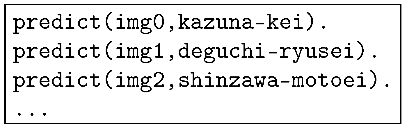
3.1.3. Logical Reasoning Mechanism

In this dataset, the logical inference machine identifies label noise data samples based on three rules as follows:

• Rule one: “One author only works for one publisher”.
• Rule two: “One author only draws manga towards one target reader”.
• Rule three: “One author only draws manga towards one genre”.

In this dataset, several authors do not satisfy these rules, and the logical inference machine not take into account them. The logical inference machine identifies label noise data samples by checking rules in first-order logic (FOL) format. To realize this, first of all, three databases: “author-publisher database”, “author-target database”, and “author-genre database” consisting of many predicates are built using SWI-Prolog [31]. The “author-publisher database” lists the publishers that each author works for, using the predicates company “company (authorA, companyB)”. The “author-target database” lists the target readers of each author (young man, girl,…), using the predicates target “target (authorA, targetB)”. The “author-genre database” lists the genre of each author (battle, sports, love-romance, etc.), using the predicates target “genre(authorA, genreB)”. Furthermore, each image in the non-expert training set also belongs to one publisher, target reader, and genre. Therefore, three other databases: “image-publisher database”, “image-target database”, and “image-genre database” are also built the same way as for authors.

During the training phase, the classification result of the temporary model, $Mode{l}_t$, is converted into predicates, as shown in Figure 6. The first argument, receiving values “img0, img1, img2”, corresponds the images included in the mini-batch data $X_t$, and the second argument, receiving values “kazuna-kei, deguchi-ryusei, shinzawa-motoei”, are the predicted names $Y_t$ of the authors that drew the corresponding images.

The Logic Inference Machine checks each image of mini-batch based on its predicted author to determine if that result violates any rules. Figure 7 shows an example for the rule one. First, the Logic Inference Machine finds the company, $Company$, that owns the image $IMG$ in the image-publisher database. It then checks if the predicted author, $Author$, works for different publishers by the predicate “workFor(Author, Company)”. This predicate returns $True$ if $Author$ works for another company, and the $IMG$ is considered violating the rule one. Other rules are similarly implemented. Each image is checked with each rule, and is added to $D_t$ if it violates one of the three rules.

3.2. Experiment on CIFAR-10

The CIFAR-10 dataset [26] includes 60,000 images belong to 1 of 10 classes (airplane, automobile, bird, cat, deer, dog, frog, horse, ship, truck). Each class includes 6000 images and be parted to 5000 images in training set and 1000 images in test set. The task is to classify the object in each image into one of the 10 classes above. The model used in image classification is ResNet14 [32].

To investigate the effective of our method, three additional labels are used to create rules: $is\_animal$ and $is\_mammal$. The detail of these label is shown in

Table 1. Additional labels for CIFAR-10 images.

	$\mathit{is}\_\mathit{animal}$	$\mathit{is}\_\mathit{mammal}$
airplane	0	0
automobile	0	0
bird	1	0
cat	1	1
deer	1	1
dog	1	1
frog	1	0
horse	1	1
ship	0	0
truck	0	0

.

The reason for that additional labels is that these images could come from various source and the place where they come from can be used as additional information. For example, the animal images come from animal albums, thus we use the label $is\_animal$ to determine whether it is animal image or not. A similar idea was used with label $is\_mammal$. An image is considered as violated sample if three additional labels of its predicted class differ with its true class.

4. Evaluation and Discussion

4.1. Accuracy

In this section, the accuracy metric is used to evaluate the performance of the aforementioned six algorithms. As shown in Equation (1), the accuracy is defined as the ratio of correct prediction samples over the whole tested data.

$$Accuracy=\frac{numberofcorrectpredictionsamples}{numberofsamples}$$

(1)

To ensure that the partitions in the train–test set do not bias the results, K-fold cross-validation (with K = 3) is used.

Table 2. Accuracy of 6 algorithms at different noise levels on Manga109.

	Noise Level	0%	20%	30%	40%	50%
Method
Normal		0.678	0.603	0.553	0.505	0.324
CF		0.679	0.597	0.422	0.411	0.303
LC-True		0.675	0.600	0.571	0.529	0.398
LC-Est		0.681	0.603	0.579	0.516	0.333
Rule-Remove		0.679	0.618	0.580	0.568	0.445
RW ($\alpha$ = 0.02)		0.679	0.619	0.568	0.551	0.419
RW ($\alpha$ = 0.1)		0.679	0.627	0.577	0.565	0.439
RW ($\alpha$ = 0.4)		0.679	0.616	0.580	0.568	0.459

and

Table 3. Accuracy of six algorithms at different noise levels on CIFAR-10.

	Noise Level	0%	20%	30%	40%	50%
Method
Normal		0.841	0.699	0.645	0.575	0.446
CF		0.824	0.678	0.625	0.565	0.435
LC-True		0.848	0.736	0.673	0.575	0.507
LC-Est		0.84	0.725	0.66	0.57	0.466
Rule-Remove		0.842	0.742	0.664	0.591	0.491
RW ($\alpha$ = 0.02)		0.835	0.739	0.666	0.585	0.466
RW ($\alpha$ = 0.1)		0.835	0.744	0.68	0.592	0.505
RW ($\alpha$ = 0.4)		0.835	0.744	0.688	0.597	0.516

show the accuracy of six algorithms when the non-expert training data contain label noise at some different level and tested with the test set.

As shown in Table 2, on Manga109 dataset, the accuracy of six algorithms decreases as the level of noise increases. When there are no noisy samples in the training set, the accuracy of all methods is nearly the same. The performances of Classification Filtering (CF) methods worsen more than the others when the noise level increases. When the noise level increases, the accuracy of Rule-Weight (SW) and Rule-Remove decreases less than the other algorithms and even better than the benchmark algorithm LC-True. The influence of the expert rules was clearly shown since the accuracy of our proposed methods denominated the Classification Filtering one.

Table 4. Label noise detection rate by expert rules on Manga109.

Noise Level	20%	30%	40%	50%
Detected label noise samples	14,704	24,561	38,799	43,060
Label noise samples	21,368	32,052	42,737	53,421
Ratio	0.689	0.766	0.907	0.806

shows the rate of label noise sample detected by the rules on Manga109 dataset. The rules can detect more than 68% of the data samples whose labels have been incorrectly assigned. This asserts that the Logic inference machine works well in detecting label noise. There was no significant difference in the accuracy between Rule-Weight and Rule-Remove. It proves that the detected label noise data samples have low weight and, thereby, low contribution to the performance of the final model.

Table 3 shows the accuracy of the algorithms for CIFAR-10 dataset. The accuracy of six algorithms decreases as the level of noise is higher and the accuracy of all methods is nearly the same when there are no noisy samples in the training set. The accuracy of Rule-Weight (SW) and Rule-Remove are the highest, and the Classification Filtering (CF) can still be the worst method as the noise level increases. These results are consistent with the ones for Manga109.

Table 5. Label noise detection rate by expert rules on CIFAR-10.

Noise Level	10%	20%	30%	40%
Detected label noise samples	1160	2357	4361	5457
Label noise samples	5000	10,000	15,000	20,000
Ratio	0.232	0.236	0.291	0.273

shows the rate of label noise sample detected by the rules on CIFAR-10 dataset. The rules just can detect 23% to 29% of the data samples whose labels have been incorrectly assigned. That explain there was no significant improvement in the performance of our proposed methods to the normal one like in Manga109 dataset.

4.2. Tuning Hyperparameters

To evaluate the effect of the learning rate ($\alpha$) of the Rule-Weight method, several values were chosen. Note that when $\alpha =0$, Rule-Weight became normal method, and Rule-Remove can be considered as a special case of RW ($\alpha =+\infty$). The results showed that at both datasets, RW ($\alpha =0.4$) outperform others, except the case there are 20% noisy label in CIFAR-10 dataset, the RW ($\alpha =0.4$) is the best. This concludes that to achieve the best performance, researchers must tune this hyperparameter base on the training phase settings (data, model) and the noise level.

4.3. Computational Complexity

The computational complexity of Rule-Remove is the same as normal method due to the cost of checking rules with first-order logic being negligible. In the Rule-Weight algorithm, because the computational cost of calculating Loss is negligible compared to the Training, the complexity of Rule-Weight is the same as the normal method.

5. Conclusions

In this paper, we propose a novel method to deal with the label noise in the dataset, which is the most important factor of a machine learning project. Using expert knowledge to detect label noise in training data, the performance of the final model is significantly improved. Two proposed algorithms can be used interchangeably to mitigate the effect of detected label noise data by adjusting the weight or removing it from the non-expert training data. In both cases, it has been that the model which is trained from the weighted dataset provides better accuracy than the original dataset. This framework can be widely applied for any machine learning algorithm without changing the structure of the model. Although the expert knowledge is in the form of first-order logic in this work, any other form of Inference Machine that can leverage expert knowledge can be used in this learning framework to detect label noise.

References

1. Frenay, B.; Verleysen, M. Classification in the Presence of Label Noise: A Survey. IEEE Trans. Neural Netw. Learn. Syst. 2014, 25, 845–869. [Google Scholar] [CrossRef] [PubMed]
2. Kuznetsova, A.; Rom, H.; Alldrin, N.; Uijlings, J.; Krasin, I.; Pont-Tuset, J.; Kamali, S.; Popov, S.; Malloci, M.; Kolesnikov, A.; et al. The Open Images Dataset V4. Int. J. Comput. Vis. 2020, 128, 1956–1981. [Google Scholar] [CrossRef] [Green Version]
3. Albarqouni, S.; Baur, C.; Achilles, F.; Belagiannis, V.; Demirci, S.; Navab, N. Aggnet: Deep learning from crowds for mitosis detection in breast cancer histology images. IEEE Trans. Med. Imaging 2016, 35, 1313–1321. [Google Scholar] [CrossRef] [PubMed]
4. Ravì, D.; Wong, C.; Deligianni, F.; Berthelot, M.; Andreu-Perez, J.; Lo, B.; Yang, G.-Z. Deep learning for health informatics. IEEE J. Biomed. Health Inform. 2016, 21, 4–21. [Google Scholar] [CrossRef] [PubMed] [Green Version]
5. Patrini, G.; Nielsen, F.; Nock, R.; Carioni, M. Loss factorization, weakly supervised learning and label noise robustness. In Proceedings of the 33rd International Conference on Machine Learning, New York, NY, USA, 20–22 June 2016; pp. 708–717. [Google Scholar]
6. Manwani, N.; Sastry, P. Noise tolerance under risk minimization. IEEE Trans. Cybern. 2013, 43, 1146–1151. [Google Scholar] [CrossRef] [PubMed] [Green Version]
7. Khardon, R.; Wachman, G. Noise tolerant variants of the perceptron algorithm. J. Mach. Learn. Res. 2007, 8, 227–248. [Google Scholar]
8. McDonald, R.A.; Hand, D.J.; Eckley, I.A. An empirical comparison of three boosting algorithms on real data sets with artificial class noise. In Proceedings of the 4th International Workshop Multiple Classifier Systems, Guilford, UK, 11–13 June 2003; pp. 35–44. [Google Scholar]
9. Melville, P.; Shah, N.; Mihalkova, L.; Mooney, R.J. Experiments on ensembles with missing and noisy data. In Proceedings of the 5th International Workshop Multi Classifier Systems, Cagliari, Italy, 9–11 June 2004; pp. 293–302. [Google Scholar]
10. Dietterich, T.G. An experimental comparison of three methods for constructing ensembles of decision trees: Bagging, boosting, and randomization. Mach. Learn. 2000, 40, 139–157. [Google Scholar] [CrossRef]
11. Zhang, C.; Wu, C.; Blanzieri, E.; Zhou, Y.; Wang, Y.; Du, W.; Liang, Y. Methods for labeling error detection in microarrays based on the effect of data perturbation on the regression model. Bioinformatics 2009, 25, 2708–2714. [Google Scholar] [CrossRef] [PubMed] [Green Version]
12. Malossini, A.; Blanzieri, E.; Ng, R.T. Detecting potential labeling errors in microarrays by data perturbation. Bioinformatics 2006, 22, 2114–2121. [Google Scholar] [CrossRef] [PubMed]
13. Kaster, F.O.; Menze, B.H.; Weber, M.-A.; Hamprecht, F.A. Comparative validation of graphical models for learning tumor segmentations from noisy manual annotations. In Proceedings of the MICCAI Workshop on Medical Computer Vision (MICCAI-MCV’10), Beijing, China, 20 September 2010; pp. 74–85. [Google Scholar]
14. Kim, H.-C.; Ghahramani, Z. Bayesian gaussian process classification with the em-ep algorithm. IEEE Trans. Pattern Anal. Mach. Intell. 2006, 28, 1948–1959. [Google Scholar] [PubMed]
15. Sun, J.-W.; Zhao, F.-Y.; Wang, C.-J.; Chen, S.-F. Identifying and correcting mislabeled training instances. In Proceedings of the Future Generation Communication and Networking, Jeju-Island, Korea, 6–8 December 2007; Volume 1, pp. 244–250. [Google Scholar]
16. Zhao, Z.; Cerf, S.; Birke, R.; Robu, B.; Bouchenak, S.; Mokhtar, S.B.; Chen, L.Y. Robust Anomaly Detection on Unreliable Data. In Proceedings of the 2019 49th Annual IEEE/IFIP International Conference on Dependable Systems and Networks (DSN), Portland, OR, USA, 24–27 June 2019; pp. 630–637. [Google Scholar] [CrossRef] [Green Version]
17. Zhu, X.; Wu, X. Class noise handling for effective cost-sensitive learning by cost-guided iterative classification filtering. IEEE Trans. Knowl. Data Eng. 2006, 18, 1435–1440. [Google Scholar]
18. Khoshgoftaar, T.M.; Rebours, P. Generating multiple noise elimination filters with the ensemble-partitioning filter. In Proceedings of the 2004 IEEE International Conference on Information Reuse and Integration, Las Vegas, NV, USA, 8–10 November 2004; pp. 369–375. [Google Scholar]
19. Brodley, C.E.; Friedl, M.A. Identifying mislabeled training data. J. Artif. Intell. Res. 1999, 11, 131–167. [Google Scholar] [CrossRef]
20. Brodley, C.E.; Friedl, M.A. Identifying and eliminating mislabeled training instances. In Proceedings of the 13th National Conference on Artificial Intelligence, Portland, OR, USA, 4–8 August 1996; pp. 799–805. [Google Scholar]
21. Ren, M.; Zeng, W.; Yang, B.; Urtasun, R. Learning to reweight examples for robust deep learning. arXiv 2018, arXiv:1803.09050. [Google Scholar]
22. Shen, Y.; Sanghavi, S. Learning with bad training data via iterative trimmed loss minimization. In Proceedings of the International Conference on Machine Learning, Long Beach, CA, USA, 9–15 June 2019; pp. 5739–5748. [Google Scholar]
23. Roychowdhury, S.; Diligenti, M.; Gori, M. Image Classification Using Deep Learning and Prior Knowledge. In Proceedings of the Workshops at the Thirty-Second AAAI Conference on Artificial Intelligence, New Orleans, LA, USA, 2–7 February 2018. [Google Scholar]
24. Matsui, Y.; Ito, K.; Aramaki, Y.; Fujimoto, A.; Ogawa, T.; Yamasaki, T.; Aizawa, K. Sketch-based manga retrieval using manga109 dataset. Multimed. Tools Appl. 2017, 76, 21811–21838. [Google Scholar] [CrossRef] [Green Version]
25. Ogawa, T.; Otsubo, A.; Narita, R.; Matsui, Y.; Yamasaki, T.; Aizawa, K. Object Detection for Comics Using Manga109 Annotations. March 2018. Available online: www.manga109.org/en/ (accessed on 9 November 2021).
26. Krizhevsky, A.; Hinton, G. Learning Multiple Layers of Features from Tiny Images; Technical Report; University of Toronto: Toronto, ON, Canada, 2009. [Google Scholar]
27. Patrini, G.; Rozza, A.; Krishna Menon, A.; Nock, R.; Qu, L. Making Deep Neural Networks Robust to Label Noise: A Loss Correction Approach. In Proceedings of the Computer Vision and Pattern Recognition (CVPR), Honolulu, HI, USA, 21–26 July 2017. [Google Scholar]
28. Thongkam, J.; Xu, G.; Zhang, Y.; Huang, F. Support Vector Machine for Outlier Detection in Breast Cancer Survivability Prediction. In Proceedings of the APWeb 2008 International Workshops, Shenyang, China, 26–18 April 2008. [Google Scholar]
29. Jeatrakul, P.; Wong, K.K.; Fung, L.C. Data Cleaning for Classification Using Misclassification Analysis. JACIII 2010, 14, 297–302. [Google Scholar] [CrossRef] [Green Version]
30. Simonyan, K.; Zisserman, A. Very Deep Convolutional Networks for Large-Scale Image Recognition. arXiv 2014, arXiv:1409.1556. [Google Scholar]
31. Wielemaker, J.; Anjewierden, A. SWI-Prolog. Available online: https://www.swi-prolog.org/ (accessed on 27 December 2019).
32. He, K.; Zhang, X.; Ren, S.; Sun, J. Deep Residual Learning for Image Recognition. In Proceedings of the 2016 IEEE Conference on Computer Vision and Pattern Recognition (CVPR), Las Vegas, NV, USA, 27–30 June 2016; pp. 770–778. [Google Scholar] [CrossRef] [Green Version]
Figure 1. Filter framework diagram.
Applsci 11 11040 g001
Figure 2. The diagram of label noise detection part and label noise processing part (Rule-Weight).
Applsci 11 11040 g002
Figure 3. The examples of Manga109 dataset. On the XML label file (a), four arguments xmin, xmax, ymin, ymax form a rectangle surrounding the object. On the image label file (b), the red, blue, yellow, and green rectangle correspond to face, body, text, and frame object.
Applsci 11 11040 g003
Figure 4. The distribution of number of samples each class in Manga109 dataset.
Applsci 11 11040 g004
Figure 5. Architecture of classification model.
Applsci 11 11040 g005
Figure 6. Logic program represents the prediction of a temporary model in first-order-logic form.
Applsci 11 11040 g006
Figure 7. Examples of rules set by expert.
Applsci 11 11040 g007