1. Introduction
The embedding of a word corresponds to a point in the continuous multidimensional real number space, and the numerical embedding brings a lot of convenience to calculation. Word embeddings contain semantics and other information learned from the large-scale corpora. Recent works have demonstrated substantial gains on many natural language processing (NLP) tasks and benchmarks by pre-training on a large corpus of text followed by fine-tuning on a specific task [
1,
2]. Thus, many machine learning methods use pre-trained word embeddings as input and achieve better performance in many NLP tasks [
3], such as the well-known text classification [
4,
5,
6] and neural machine translation [
7,
8,
9], among others.
One of the earliest studies on word representations dates back to 1986 and was conducted by Rumelhart, Hinton, and William [
10]. In the following decades, many word embedding models based on the bag-of-words (BOW) language model (LM) and neural network LM have been proposed. These word embedding models include the well-known LDA [
11], Word2Vec [
12], Glove [
13], ELMO [
14], and BERT [
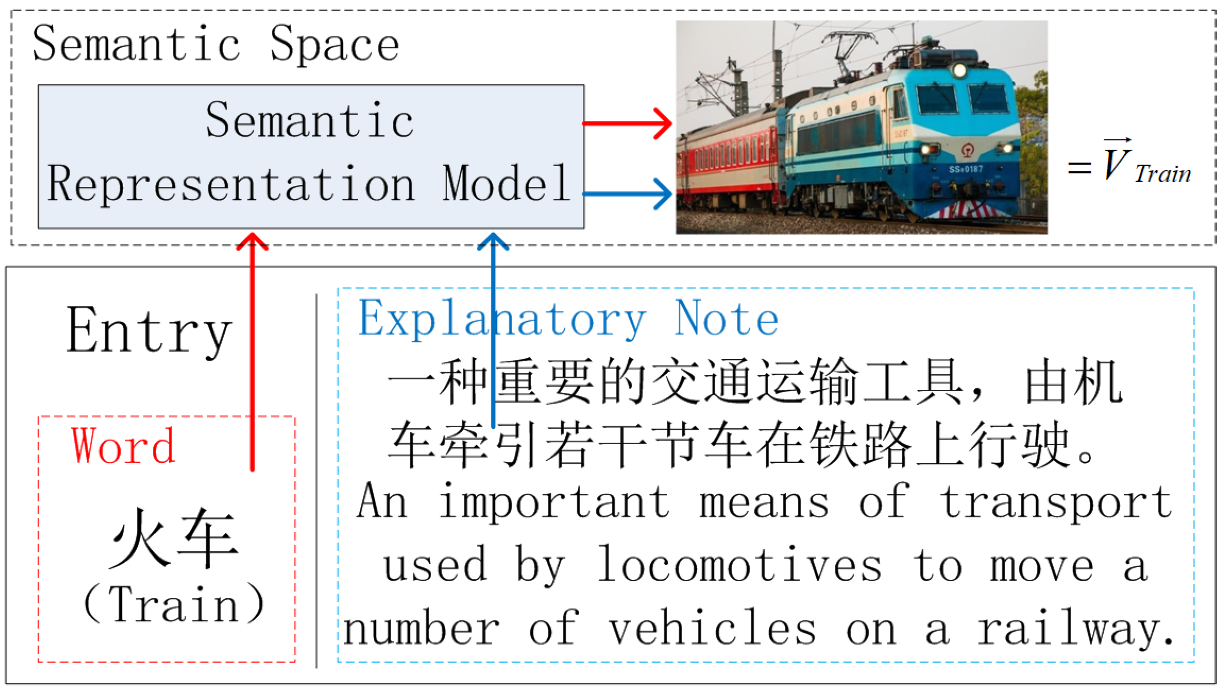
1]. As soon as BERT was proposed, it outperformed the state-of-the-art methods on eleven NLP tasks. Usually, these word embedding models are trained using a huge corpus. However, for some low-resource languages, it is infeasible to construct a large corpus. When using a small corpus to estimate word embeddings, sparsity is a major problem. Sparsity leads to out-of-vocabulary (OOV) everywhere. For some tasks that require word segmentation, the OOV phenomenon is more obvious. This is because word segmentation leads to more significant long-tail characteristics [
15,
16]. In addition, Zipf’s law applies to most languages. This makes word embedding models unable to fully learn the semantics of OOVs and low-frequency words [
16,
17]. Therefore, accurately estimating the embeddings of OOVs and low-frequency words becomes the research motivation of this paper. We take Chinese as an example and use a dictionary to estimate the embeddings of those words. Different from English texts, there are no explicit delimiters such as whitespace to separate words in Chinese texts [
15,
18], just like the explanatory note in
Figure 1. Therefore, Chinese word segmentation is important for some Chinese NLP tasks [
15,
18]. However, Chinese word segmentation will cause more serious sparsity problems, which makes the embeddings of OOVs and low-frequency words more difficult to be estimated [
16].
An entry in the dictionary contains a word and the corresponding explanatory note. They all point to the same point in the semantics space. As shown in
Figure 1, the explanatory note usually contains rich information which explains the meaning of the corresponding word exactly. Inspired by this, we designed a semantics extractor to extract semantics from explanatory notes. We use the semantics representation produced by the extractor as the representation of low-frequency words. For high-frequency words, we still retain their word representations estimated by other word embedding models, such as Word2Vec. By combining the two types of word embedding estimation methods, we will obtain higher quality word representations that will be fine-tuned in downstream tasks. As the extrinsic experimental results in this paper show, the higher the quality of the word representation, the better the performance we will obtain. Our main contributions are as follows:
2. Related Work
Our work mainly involves the estimation of OOVs and low-frequency words’ embeddings and designing a sentence representation model. In this section, we introduce the related works of these two aspects.
Whether it is static word embedding models such as Word2Vec, Glove, and fasttext [
12,
13,
21], or dynamic word embedding models such as BERT, ELMO, and GPT [
1,
2,
14], they all extract features from a large number of samples to generate word representations. For OOVs that have never appeared and low-frequency words, these models are unable to estimate their representation well [
17]. Researchers have studied how to improve the estimate of OOVs and low-frequency words’ representations. These methods mainly use the surface features of OOVs and their context to predict the meaning. Three types of embeddings (word, context clue, and subword embeddings) were jointly learned to enrich the OOVs’ representations [
22]. In [
17], an OOV embedding prediction model named hierarchical context encoder (HiCE) was proposed to capture the semantics of context as well as morphological features. Recently, a mimicking approach has been found to be a promising solution to the OOV problem. In [
23], an iterative mimicking framework that strikes a good balance between word-level and character-level representations of words was proposed to better capture the syntactic and semantic similarities. In [
24], a method was proposed to estimate OOVs’ embeddings by referring to pre-trained word embeddings for known words with similar surfaces to target OOVs. In [
25], the embeddings of OOVs were determined by the spelling and the contexts in which they appear. The above-mentioned word embedding models that use morphology to infer the representations of OOVs are effective for English. However, they are not necessarily effective for Chinese, because many words with similar forms have very different meanings.
An explanatory note in an entry is usually a complete sentence. We naturally think of using the sentence representation model to extract the semantics from the explanatory note and treat it as the semantics of the corresponding word. In recent years, many sentence representation models have been proposed and widely used. Facebook AI’s fasttext is a sentence representation model based continuous skip-gram model [
12,
21], which can estimate both word representations and sentence representations (
https://github.com/facebookresearch/fastText, accessed on 5 March 2021). In [
26], an unsupervised sentence embedding method (sent2vec) using compositional n-gram features was proposed to produce general-purpose sentence embeddings. Both fasttext and sent2vec are all BOW models, and we think that the BOW mechanism is just the simple combination of word embeddings. BERT is a landmark dynamic word embedding model. It learns sentence representations by performing two tasks: masked word prediction (MWP) and next sentence prediction (NSP) [
1]. The embedding of token [CLS] in the last layer of BERT is considered as the representation of the input sentence. SBERT-WK is a sentence representation model based on BERT. It calculates the importance of words in sentences through subspace analysis and then weights word embeddings to generate sentence representations [
27]. In [
28], the framework of neural machine translation (LASER) was adopted to jointly learn sentence representations across different languages. BERT uses a bidirectional self-attention encoder (the transformer) to encode sentences, and LASER uses a BiLSTM. In addition, there are more studies on sentence representations [
29,
30,
31].
There are many publicly available sentence representation models. [
1,
21,
26,
27,
32]. However, so far, there is no sentence representation model without any flaws. BERT only uses the embedding of [CLS] in the last layer of BERT to represent the input sequence [
1]. The embedding of [CLS] is mainly learned from NSP. However, a recent study shows that NSP does not contribute much to the sentence representation learning [
33]. SBERT-WK can make use of the existing semantics in BERT as much as possible, but it cannot increase the semantics in BERT. LASER is a universal multilingual sentence representation model covering more than 100 languages [
32], and it uses BiLSTM to encode sentences. We believe that there are some limitations to constructing a large and high-quality parallel corpus, and the encoding ability of BiLSTM is also inferior to Transformer. sent2vec and fasttext are BOW LMs, and they both use the n-gram features to represent the semantics of sentences [
21,
26]. Thus, in this article, we propose a new sentence representation model from a new perspective.
3. Lessons Learned from an Infeasible Heuristic Model
In this section, we introduce lessons learned from an infeasible heuristic model. The lessons guide us to construct our new sentence representation model.
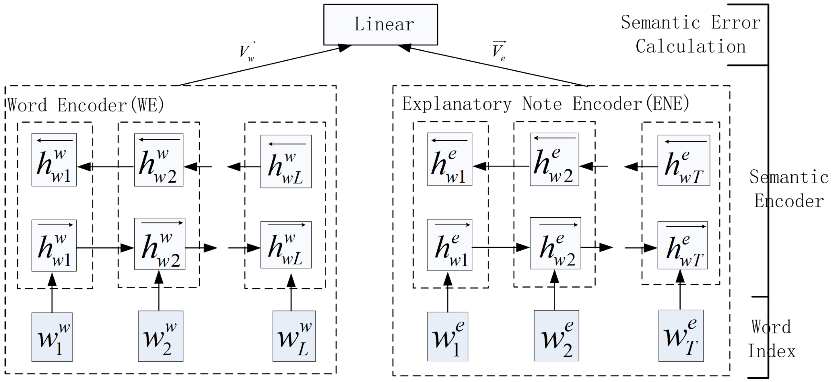
As
Figure 1 shows, an entry consists of a word and its explanatory note. A word and its explanatory note all point to the same point in the semantics space. The natural idea is to construct two different encoders to encode the word and its explanatory note. The two encoders shown in
Figure 2 are trained with the goal of minimizing the difference of the two outputted semantics vectors. WE and ENE do not share parameters, and they both use a BiLSTM or BiGRU to encode the token sequence. The detail of the encoder can be seen in [
34].
Suppose we have an entry
.
and
which represent a word and its explanatory note in an entry. We use
and
to denote the semantics vectors of the word and the explanatory note. We use the euclidean distance (or the cosine distance) to measure the semantics difference between the two vectors. To make the semantics difference as small as possible, we design the objective function defined by Equation (
1) and minimize it to train WE and ENE shown in
Figure 2.
So far, everything seems to be going according to our expectations. Unfortunately though, no matter how we jointly train WE and ENE, the parameters being trained always converge to
0. The output of WE and ENE also tend to
, that is, the semantics vector we finally obtain tends to
. Why? Because
0 is one of the feasible solutions of the model, and 0 is the minimum loss of the objective function defined by Equation (
1). With the effective search of optimization algorithm (we use Adam [
35] to optimize the model), the loss of the objective function tends to 0 finally, and the parameters being trained also tend to
0. Therefore, we can conclude that we cannot approximate an implicit objective that varies with optimization parameters because such implicit objectives make the loss function of the model have zero solutions, and when the loss function is equal to 0, all parameters are zero. This is why pre-trained LMs such as Word2Vec, BERT, XLNet, and GPT [
1,
2,
12,
19] all regard words in the vocabulary as prediction targets (the predicted words are fixed and will not vary with the trainable parameters). Based on this principle, we design a new sentence representation model.
4. The Proposed Sentence Representation Model
As
Figure 1 shows, an entry consists of a word and the corresponding explanatory note. Usually, an explanatory note is a complete sentence, so we extract the semantics of the explanatory note and treat it as the representation of the corresponding word.
We use
to represent a sentence with length
m. The sentence representation of
is denoted by
. We assume that the more tokens a sentence contains, the more semantics it conveys. Let us consider two token sequences,
and
.
has one more token
than
. According to the hypothesis,
contains more semantics than
. The added semantics of
than
is mainly caused by
, so we can use the added semantics to predict
, that is,
In Equation (
2), the sentence representation
is calculated by the self-attention mechanism. The self-attention mechanism in our sentence representation model shown in
Figure 3 is slightly different from the traditional self-attention mechanism [
1]. Suppose that
is the output of the encoder when the input token sequence is
.
is the encoding of
. The calculation process of the sentence representation of
is shown in
Figure 3.
In
Figure 3,
,
, and
b represent the query vector, the shape transformation matrix, and the bias, respectively. The
e,
, and ⊙ operations are all element-wise.
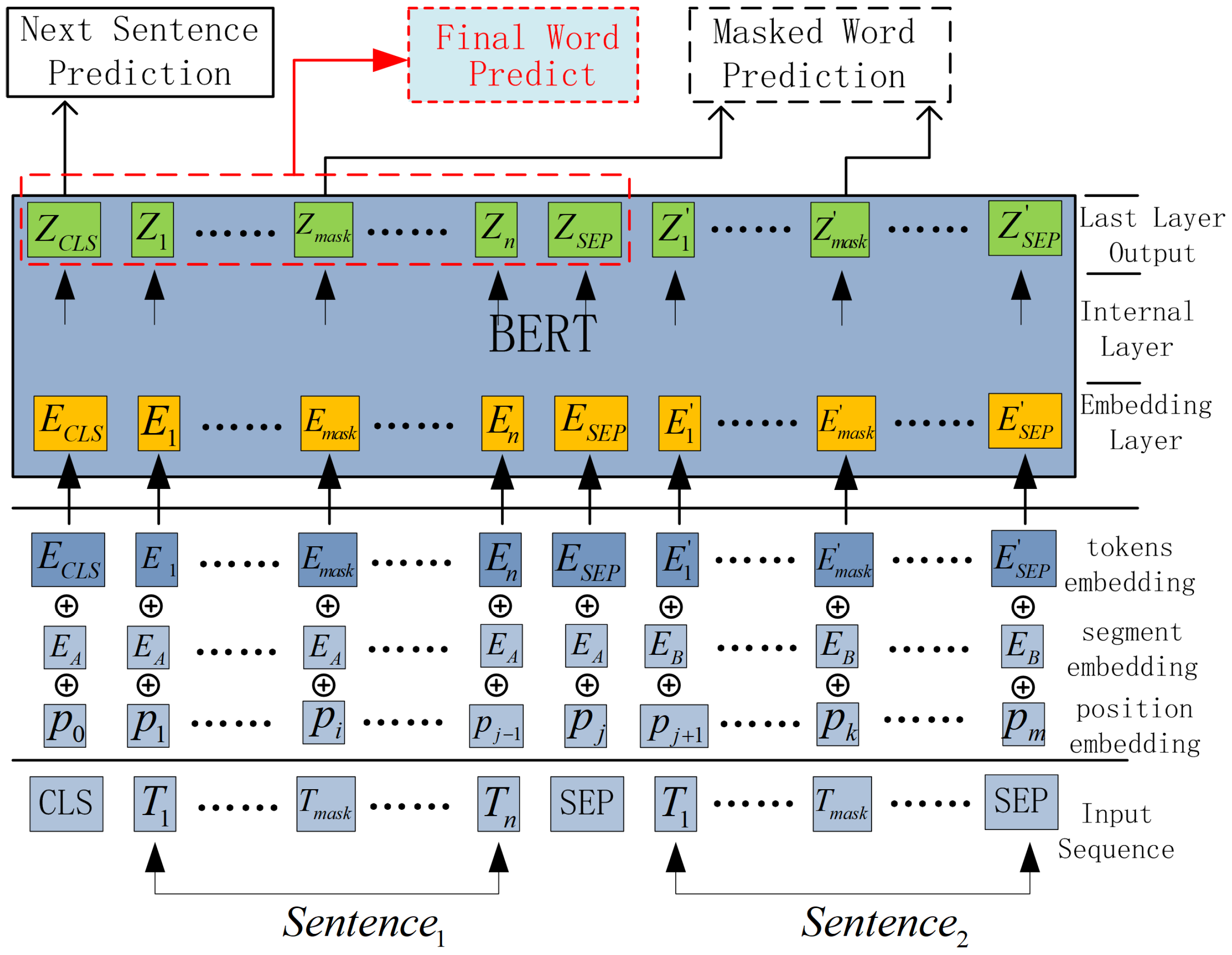
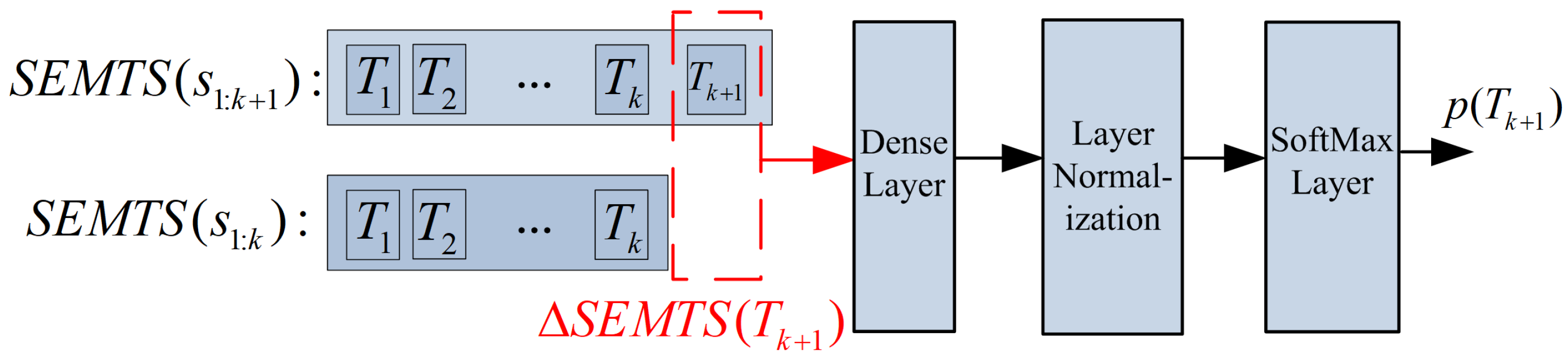
To make full use of the strong encoding ability of BERT, we use BERT as the backbone of our sentence representation model. Another benefit of building and fine-tuning the model based on BERT is that it can save a lot of computation power. Thus, we add our semantics computing module to BERT as a sub-task, and we call our semantics representation model SEMTS-BERT. The architecture of SEMTS-BERT is shown in
Figure 4. NSP and MWP are two sub-tasks of the original BERT [
1]. Final Word Prediction (FWP) sub-task corresponds to our semantics computing model, and its structure is shown in
Figure 5. The loss of FWP sub-task is defined as
where
is the probability of
defined in Equation (
2) when using the added semantics to predict
.
N is the number of predicted words in a batch.
is calculated by FWP, shown in
Figure 5. When we minimize the objective, the loss of FWP defined in this way makes the probability of predicted words as large as possible.
The total loss of SEMTS-BERT is the sum of
,
, and
, that is,
The detail of
and
can be seen in [
1].
5. Experiment
In this section, we choose Chinese as a study case and perform two types of experiments: intrinsic evaluation and extrinsic evaluation [
17]. The intrinsic evaluation is designed to evaluate the effectiveness of our proposed SEMTS-BERT. It includes three tasks: a probing task [
36], a text classification task, and a Natural Language Inference (NLI) task. The extrinsic evaluation is designed to verify the quality of OOVs and low-frequency words’ embeddings. In the extrinsic experiment, we replace OOVs and low-frequency words’ embeddings in two downstream tasks: sentence semantic equivalence identification (SSEI) and question matching (QM) [
37,
38]. We also evaluate the quality of low-frequency words’ embeddings by investigating the relative distance between similar words.
5.1. Experimental Settings
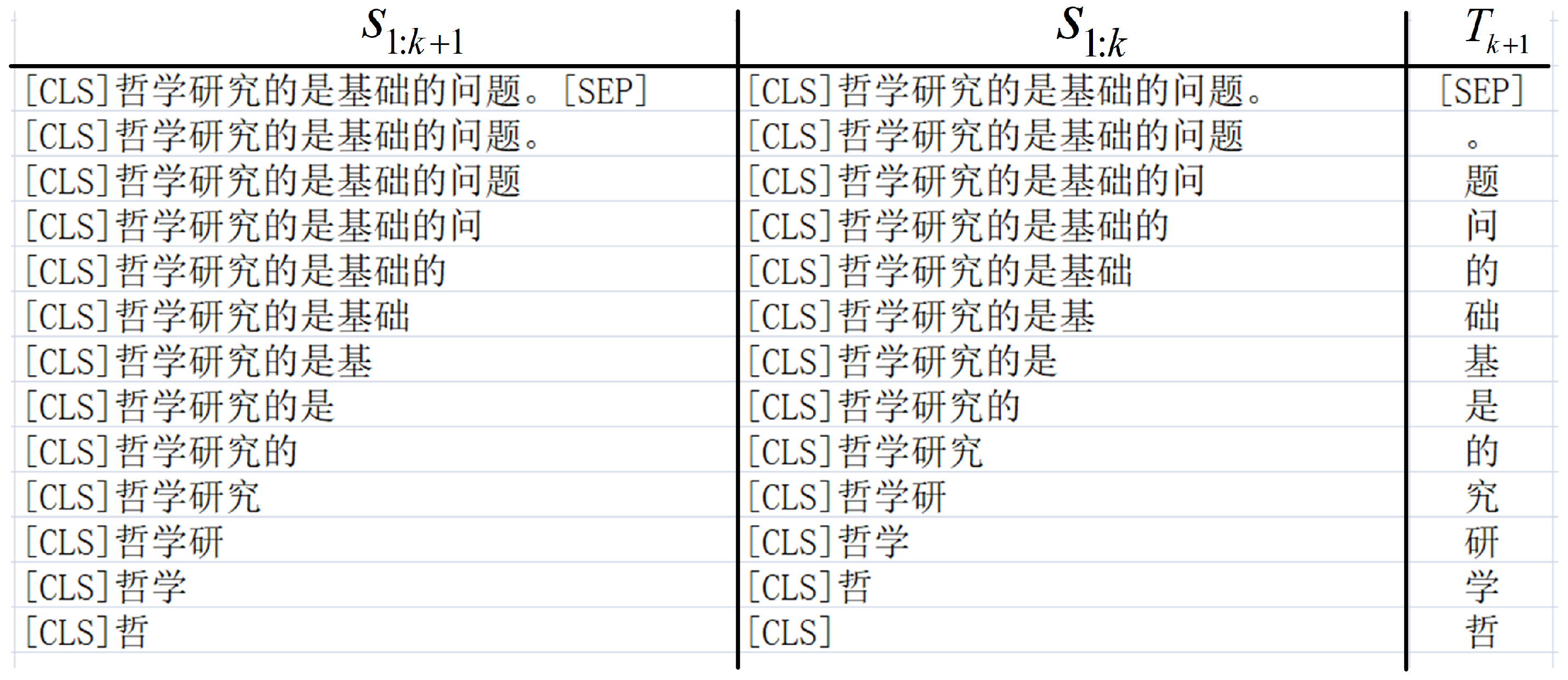
As shown in
Figure 4, our model is composed of FWP module and BERT. We initialize our model with the Chinese 12-layer, 768-hidden, 12-head, 110M parameter BERT-Base model (
https://github.com/google-research/bert, accessed on 10 March 2021) and train it with a dataset derived from texts (250M bytes) downloaded from Wikipedia (
https://dumps.wikimedia.org/zhwiki/, accessed on 1 June 2020). We take a Chinese sentence “哲学研究的是基础的问题。” (“Philosophy studies basic issues”) as an example to illustrate the construction of the dataset. We use the Adam optimizer (the initial learning-rate and the warm-up steps are set to
and 12,000) to train SEMTS-BERT 2 epochs [
35]. The batch size is 2 and the maximum sequence length is set to 128. As shown in
Figure 6, a sentence can derive many examples. We can obtain nearly 200 examples when the batch size and the maximum sequence length are set to 2 and 128. When SEMTS-BERT has been trained, we use the process shown in
Figure 3 to calculate sentences’ representation. For an entry in dictionaries, we input the explanatory note into SEMTS-BERT, and the output is the representation of the corresponding word.
5.2. Baselines
We choose the following models as baselines to evaluate the performance of SEMTS-BERT. The performance of sentence representation models directly determines the quality of low-frequency words’ embeddings.
BERT: In addition to estimating dynamic word embedding, BERT can also be used to calculate the embedding of a sentence (the encoding of [CLS] in the last layer is treated as the sentence representation) [
1].
fasttext
https://fasttext.cc/, accessed on 7 March 2021: fasttext is a pre-training BOW model for 157 different languages. It is a famous library for estimating both words and sentences [
21].
sent2vec
http://github.com/epfml/sent2vec, accessed on 7 March 2021: sent2vec is an efficient unsupervised BOW model, and it uses word embeddings and n-gram embeddings to estimate sentence representations [
26].
LASER
https://github.com/facebookresearch/LASER, accessed on 8 March 2021: LASER is a multilingual sentence representation model. It adopts BiLSTM as an encoder which was trained on a parallel corpus that covers 93 languages [
28].
SBERT-WK: SBERT-WK is a sentence representation model based on BERT. It calculates the importance of words in sentences through subspace analysis and then weights the word embeddings to obtain sentence representations [
27].
5.3. Intrinsic Evaluation 1: Evaluate SEMTS-BERT on Probing Tasks
Probing tasks are designed to evaluate the performance of models on capturing the simple linguistic properties of sentences [
39]. We use the Chinese CoNLL2017 (
http://universaldependencies.org/conll17/data.html, accessed on 7 June 2020) for this evaluation. The dataset is uneven, and its statistics are shown in
Table 1. We adopt some sub-tasks defined in [
36,
39] in our evaluation. They are:
Sentence_Len (sentence length): We divide sentences into two classes: class 0 (its length is shorter than the average length) and class 1 (its length is longer than the average length). In this test, the classifier is trained to tell whether a sentence belongs to class 0 or 1.
Voice: The goal of this binary classification task is to test how well the model can distinguish the active or passive voice of a sentence. In the case of complex sentences, only the voice of the main clause is detected.
SubjNum: In this binary classification task, sentences are classified by the grammatical number of nominal subjects of main predicates. There are two classes: sing and plur.
BShift: In the BShift dataset, we exchange the positions of two adjacent words in sentence. In this binary classification task, models must distinguish intact sentences from sentences whose word order is illegal.
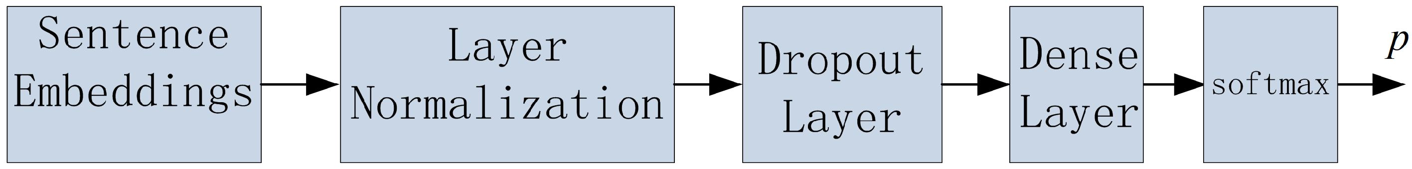
In this test, we fit a Multi-Layer Perception (MLP) with one hidden layer on the top of the sentence representation model to perform the classification [
40]. The architecture of MLP is illustrated in
Figure 7.
5.3.1. Experimental Results
The experimental results of probing tasks are shown in
Table 2. We use accuracy to express the performance since
in classification.
P,
R, and
F represent precision, recall, and
F-measure:
,
,
. We use the mean and standard deviation (number in brackets) to express the performance of models.
means that the encoding of the token [CLS] is treated as the representation of the input sentence.
means that the max-pooling of the encodings in BERT’s last layer is treated as the representation of the input sentence, and
means that the mean-pooling of the encodings in BERT’s last layer is treated as the representation of the input sentence.
and
are the same as
and
.
represents the native sentence representation model of fasttext. We input the embeddings of sentences into the classifier described in
Figure 7 to evaluate each sentence representation model.
From
Table 2, we can see that
performs best on Bshift and subjNum but worst on Sentence_Len. SEMTS-BERT and
perform best on Sentence_Len and Voice. In the Voice sub-task, all models achieve good performance. In Bshift, all models except
do not perform well. Among all the models, the standard deviation of
is the largest, which shows that its training results are unstable and tend to fall into the local extremum easily during the optimization process. We try to reduce the number of neurons in the hidden layer to reduce
’s standard deviation, but doing so will reduce its overall performance. Compared with the native sentence representation model, max and mean pooling operations sometimes achieve better performance.
5.3.2. Analysis and Conclusion
SEMTS-BERT has the best overall performance, followed by SBERT-WK and
. Compared with
,
, and
, the performance of
has been proven to be the best in probing tasks [
36]. This shows that SEMTS-BERT has good performance on probing tasks. Due to the self-attention mechanism, SEMTS-BERT cannot retain the positional relationship of tokens well, but its performance on Bshift is still better than
,
, and
.
performs best on Bshift because it can obtain the token position information from residual connections between layers and local features from the masked LM [
1]. From Bshift, we can draw a conclusion that the weighted operation cannot filter all the positional information.
and
are based on the BOW LM, so it is easy to understand that they do not perform well on this task. However, LASER uses BiLSTM to encode token sequences, and it should be sensitive to the word order, but the experimental results are not the same as our expectation.
5.4. Intrinsic Evaluation 2: Evaluate SEMTS-BERT on Text Classification
Text classification is a popular task used to evaluate the performance of models in NLP [
5]. In this section, we evaluate the performances of different sentence representation models on three Chinese text classification datasets.
Thucnews: A high-quality 14-category text classification dataset containing 0.74M news articles collected from Sina News:
https://news.sina.com.cn/, accessed on 1 May 2021. The dataset is provided by the NLP Laboratory of Tsinghua University:
http://thuctc.thunlp.org/, accessed on 1 May 2021.
Fudan Dataset (Fudan): Fudan dataset:
http://www.nlpir.org/?action-viewnews-itemid-103, accessed on 1 May 2021, is a 20-category text classification dataset that contains 9833 test documents and 9804 training documents. It is an uneven dataset since the number of documents of each category varies greatly.
TouTiao Dataset (TouTiao): TouTiao dataset is a 15-category short text classification dataset. Each example contains only a news headline and a subheading. It is noisy and collected from TouTiao news website:
www.toutiao.com, accessed on 1 May 2021.
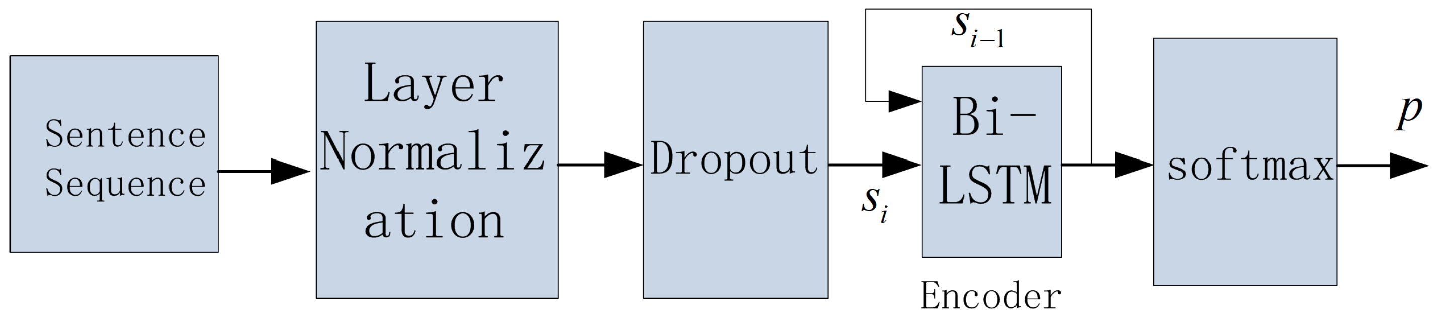
We first split paragraphs into sentences and the calculate the representations of sentences. We later use a BiLSTM encoder to encode the sentence representation sequence. Finally, the outputs of the encoder (document representations) are inputted into the softmax layer to perform text classification. The architecture of the text classifier is shown in
Figure 8. We use the Adam optimizer [
35] to train each model 50 epochs with early stop strategy on every dataset.
5.4.1. Experimental Results
We list the experimental results of this evaluation in
Table 3.
,
, and
have the same meaning as those in
Table 2. We can easily see that our SEMTS-BERT performs best. The variance of BERT and fasttext on Toutiao and Thucnews is very large, which shows that the text classification results of these two models are unstable. Due to the vagueness and ambiguity of some examples in Toutiao, the classification accuracy of all models on Toutiao is not high, and the results are not stable.
5.4.2. Analysis and Conclusions
Our model obtains the best performance on this test. This shows that our sentence encoding mechanism can represent the semantics of sentences well. The overall performance of BERT model is worst, which shows that BERT needs further fine-tuning to obtain better performance in downstream tasks (sentence embeddings are fixed in this text). has achieved second only to us, and its performance has surpassed LASER. This shows that in text classification, a simple BOW model can also perform well. Compared with BERT, SBERT-WK achieves better performance, which indicates that the sentence representation obtained by weighting the embeddings in each layer has better performance than using only the output of the last layer as the sentence representation.
5.5. Intrinsic Evaluation 3: Evaluate SEMTS-BERT on Natural Language Inference (NLI)
In NLI task, a classifier is trained to determine whether one sentence entails, contradicts another sentence, or neither [
41]. We use the Chinese XNLI corpus for this test [
41]. The Chinese XNLI dataset contains 2312 and 4666 sentence pairs in its development set and test set. We randomly re-divide them into train, development, and test sets. The classifier used in this test is shown in
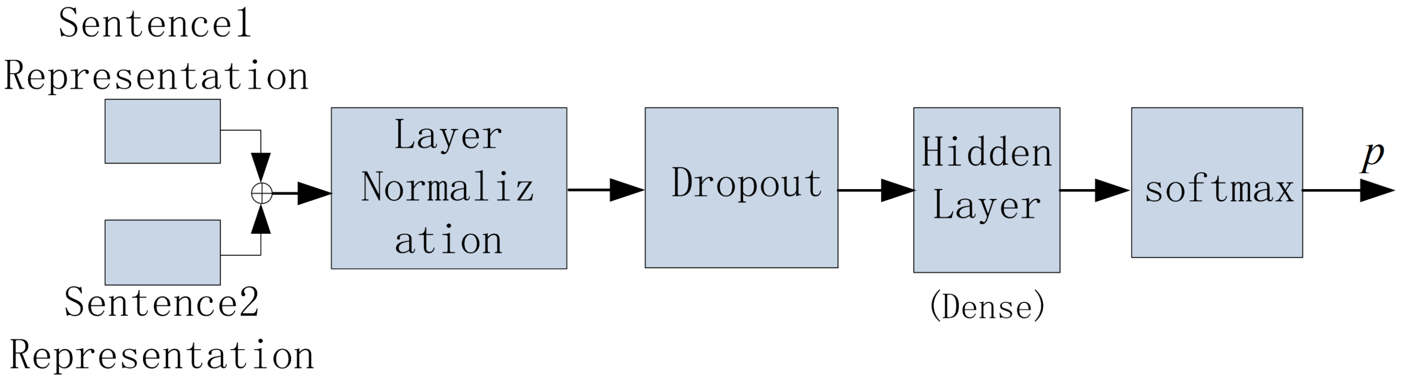
Figure 9. ⊕ represents the concatenation of the two vectors.
5.5.1. Experimental Results
The experimental results of the Chinese NLI are shown in
Table 4. The meanings of
,
, and
are the same as those in
Table 2. LASER performs the best, followed by our model. The standard deviation of
is very large, which shows that the classifier can easily fall into a local extremum during the training process. The
models of
and
perform better than
and
models. This shows that the native sentence models are more suitable to the NLI task than the pooling models. The
model performs better than the
model. The same conclusion is obtained in [
36].
5.5.2. Analysis and Conclusion
BiLSTM can encode sequences well [
42]. LASER uses a BiLSTM to encode token sequences, and it is trained on a large multilingual parallel corpus [
32]. Therefore, it is understandable that it performs best, and the same conclusion has also been drawn in [
36]. BERT uses a Transformer-based bidirectional encoder to encode the sequence [
1]. In this test, the performance of BERT is not as good as LASER. This is because the sentence embeddings are fixed, and BERT can not benefit from the larger, more expressive pre-training representations [
1]. However, our sentence representation model can improve this situation.
and
have the worst performance. They both use a BOW LM to represent the semantics of sentences [
21,
26]. The sequence encoding ability of BOW is obviously inferior to BiLSTM and Transformer [
36]. Surprisingly, the performance of SBERT-WK is not as good as
and
. This shows that the complex weighting operation in SBERT-WK cannot improve the NLI performance of BERT. Because we only use simple classifier and the sentence representations are fixed, the optimal performance in this test is not high. However, this is enough for us to compare the semantics representation abilities of different models.
5.6. Extrinsic Evaluation 1: Evaluate the Quality of Low-Frequency Words’ Embeddings by the Relative Distance
In this evaluation, we assume that in a set of words with similar meanings, if their embeddings are more concentrated, the quality of their embeddings will be better. We choose nine Chinese low-frequency words with similar meanings for this evaluation. They are 砂仁 (Fructus Amomi), 腽肭脐 (Testiset Penis Phocae), 枳壳 (Fructus Aurantii), 枳实 (Fructus), 紫河车 (Placenta Hominis), 阿胶 (Donkey-Hide Gelatin), 白药 (Baiyao, a white medicinal powder for treating hemorrhage, wounds, bruises, etc.), 膏药 (Plaster), 槐豆 (Locust Bean). These words are the names of some traditional Chinese medicines.
We use Word2Vec (trained on the Chinese text corpus downloaded from Wikidata) to estimate the embeddings of these words. We use SEMTS-BERT, SBERT-WK, and LASER to calculate the embedding of the explanatory note and regard the embedding as the embedding of the corresponding word. For example, the explanatory note of 砂仁 in the dictionary is “阳春砂或缩砂密的种子, 入中药, 有健胃、化滞、消食等作用”. We input this explanatory note into a sentence representation model, and the produced embedding is treated as the embedding of 砂仁.
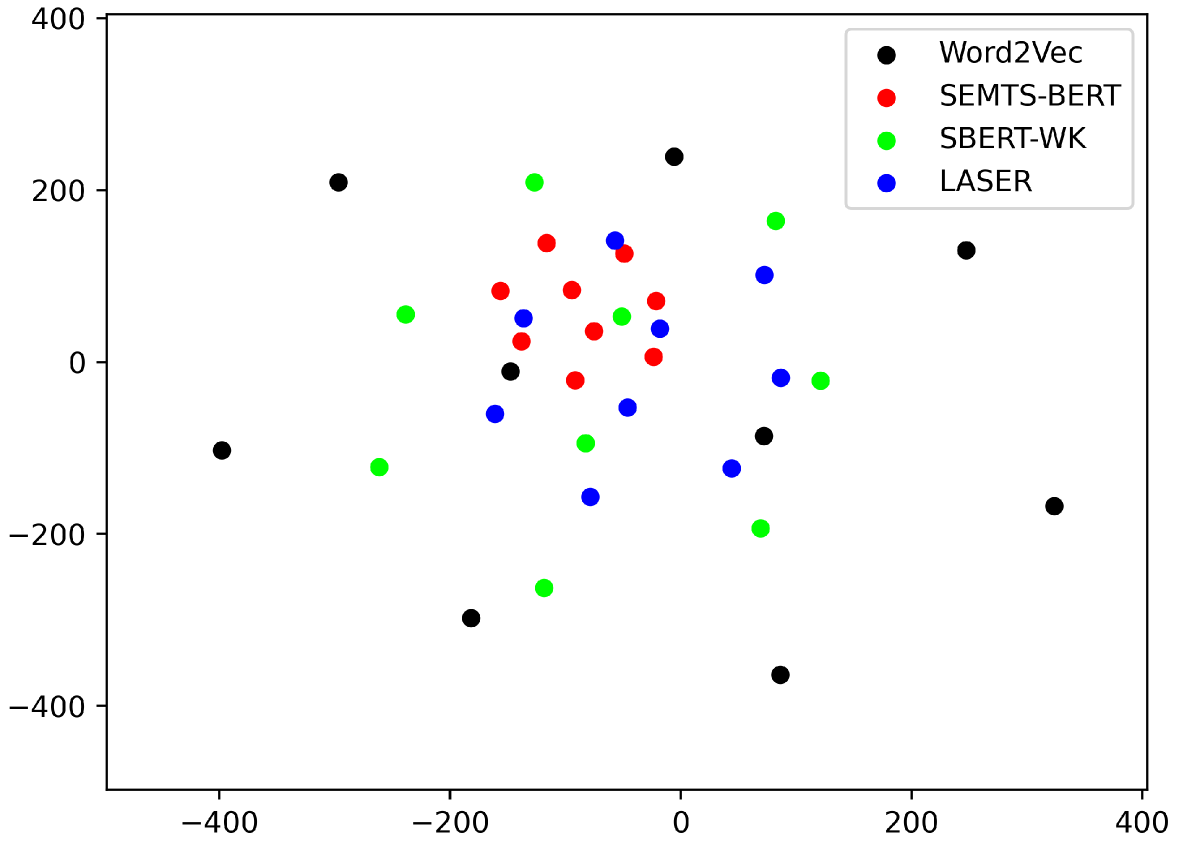
The relative distances between the nine Chinese low-frequency words are shown in
Figure 10. The embeddings estimated by our model have a smaller relative distance. Therefore, we think that our method can produce higher-quality low-frequency word embeddings.
5.7. Extrinsic Evaluation 2: Evaluate the Quality of Low-Frequency Words’ Embeddings on Downstream Tasks
We assume that the higher the quality of word embeddings, the better the performance we will obtain. Based on this assumption, we indirectly evaluate the quality of word embeddings through the performance of specific tasks. We adopt SSEI (sentence semantic equivalence identification) and QM (question matching) to evaluate the performance improvement caused by replacing the embeddings of low-frequency words [
37,
38]. By replacing the embeddings of OOVs and low-frequency words in train, development, and test sets, we can evaluate whether our proposed low-frequency word embedding estimation method can improve the performance of SSEI and QM as well as how much the performance has been improved. From the improvement, we can determine whether the quality of low-frequency words’ embeddings has been improved.
5.7.1. Experimental Design
We use the Chinese dictionary named XIANDAI HANYU CIDIAN and choose two NLP tasks (SSEI and QM) for this evaluation. SSEI is a fundamental task of NLP in question answering (QA), automatic customer service, and chatbots. In customer service systems, two questions are defined as semantically equivalent if they convey the same intent or they could be answered by the same answer. Because of rich expressions in natural languages, SSEI is a challenging NLP task [
37]. QM is also a fundamental task of QA, which is usually recognized as a semantic matching task, sometimes a paraphrase identification task. The goal of QM is to search questions that have similar intent as the input question from an existing database [
38].
Without replacing the OOVs and low-frequency words’ embeddings in train, development, and test sets, we first evaluate the performance of the baseline sentence matcher on the two datasets. We later replace low-frequency words’ embeddings in the same dataset, and we evaluate the performance of the baseline sentence matcher again. By comparing the two results, we can obtain the performance improvement and determine whether our proposed method improves the quality of low-frequency words’ embeddings. We use Word2Vec (
https://github.com/RaRe-Technologies/gensim, accessed on 10 June 2021) to estimate word embeddings on a large Chinese corpus downloaded from Wikidata [
12]. We use SEMTS-BERT, SBERT-WK, and LASER to estimate OOVs and low-frequency words’ embeddings. When we input the explanatory note of an entry (suhc as the one shown in
Figure 1) into a sentence representation model, the outputted sentence representation is considered as the embedding of the corresponding word. We choose LASER and SBERT-WK for the comparison because they have been proven high-performance [
27,
36].
5.7.2. Datasets
We use BQ [
37] and LCQMC [
38] datasets for this evaluation. Each example in BQ and LCQMC contains a sentence pair and a label. The label indicates whether the two sentences in sentence pairs match. The train, development, and test sets of BQ contain 100k, 10k, and 10k examples, respectively, and the train, development, and test sets of LCQMC contain 238k, 8.8k, and 12.5k examples, respectively. We use jieba (
https://pypi.python.org/pypi/jieba, accessed on 1 July 2021) to perform Chinese word segmentation. The distributions of low-frequency words of the two datasets are shown in
Table 5.
5.7.3. Baseline and Parameter Settings
We choose BiLSTM, Text-CNN, DCNN, DIIN, BiMPM, and other machine learning models as sentence matcher baselines [
44,
45,
46,
47,
48]. BiMPM is a character+word model [
46], and it obtains the best results on BQ and LCQMC. The embeddings of characters are tuned, and the embeddings of words can be dynamic (tuned) or static (not to be tuned) in the evaluation.
5.7.4. Experimental Results
The comparisons between our model and other models on BQ and LCQMC are shown in
Table 6 and
Table 7,
Appendix A and
Appendix B. “c” and “w” in the
Emb column represent the character-based and the word-based model. “Acc.” represents the classification accuracy. “+st.” and “+dy.” denote that word embeddings are fixed and to be tuned during the training. “+LASER”, “+SB-WK”, and “+SEMTS” mean that the embeddings used to replace the original embeddings of low-frequency words are calculated by LASER, SBERT-WK, and SEMTS-BERT, respectively. On both BQ and LCQMC, we all use the word-based BiMPM. On the BQ dataset, we obtain the similar performance to the benchmark obtained by a character-based model [
37]. Generally, the performance of character-based model is better than the performance of word-based model on small Chinese datasets due to sparsity [
16]. On the LCQMC dataset, we achieve better performance than the benchmark.
From
Table 6 and
Table 7,
Appendix A and
Appendix B, we can draw a conclusion that we achieve better performance when we replace the low-frequency words’ embeddings on the larger LCQMC dataset. The performance of the word-based model exceeds that of the character-based model after performing the replacement. This shows that we can obtain higher-quality word embeddings through the proposed method when the dataset is large. On the smaller BQ dataset, the replacement also promotes the word-based model. Sometimes, the performance of word-based models exceeds that of the character-based model after performing the replacement. In summary, the performance improvement indicates that our method can provide higher-quality low-frequency words’ embeddings.
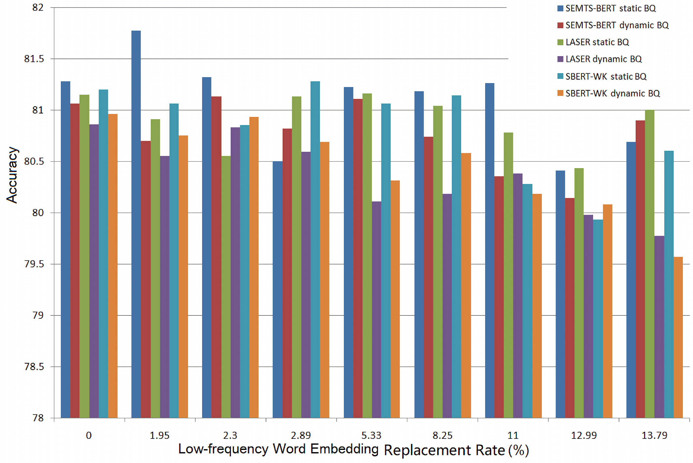
Figure 11 and
Figure 12 show the experimental results on BQ and LCQMC at different low-frequency word embedding replacement rates. The bars “SEMTS-BERT *” represent the accuracy of BiMPM at different low-frequency word embedding replacement rates when SEMTS-BERT is used to estimate the embeddings. The bars “LASER *” and “SBERT-WK *” also have similar meanings. “Static” and “dynamic” indicate that word embeddings are fixed and to be tuned during the training. When the low-frequency word embedding replacement rate is 0, we did not use the word embeddings calculated by the sentence representation model to replace the original word embeddings estimated by Word2Vec.
It can be seen from
Figure 11 that when using LASER and SBERT-WK to estimate OOVs and low-frequency words’ embeddings, the replacement cannot improve the accuracy of BiMPM on BQ, no matter if the embeddings of words are static or dynamic. When using SEMTS-BERT to estimate OOVs and low-frequency words’ embeddings and the embeddings of words are fixed during the evaluation, the replacement of low-frequency words’ embeddings can improve the accuracy of the word-based BiMPM at the replacement rate of 1.95% (from 81.28% to 81.77%). When word embeddings are dynamic, SEMTS-BERT can not improve the performance of the word-based BiMPM on BQ either.
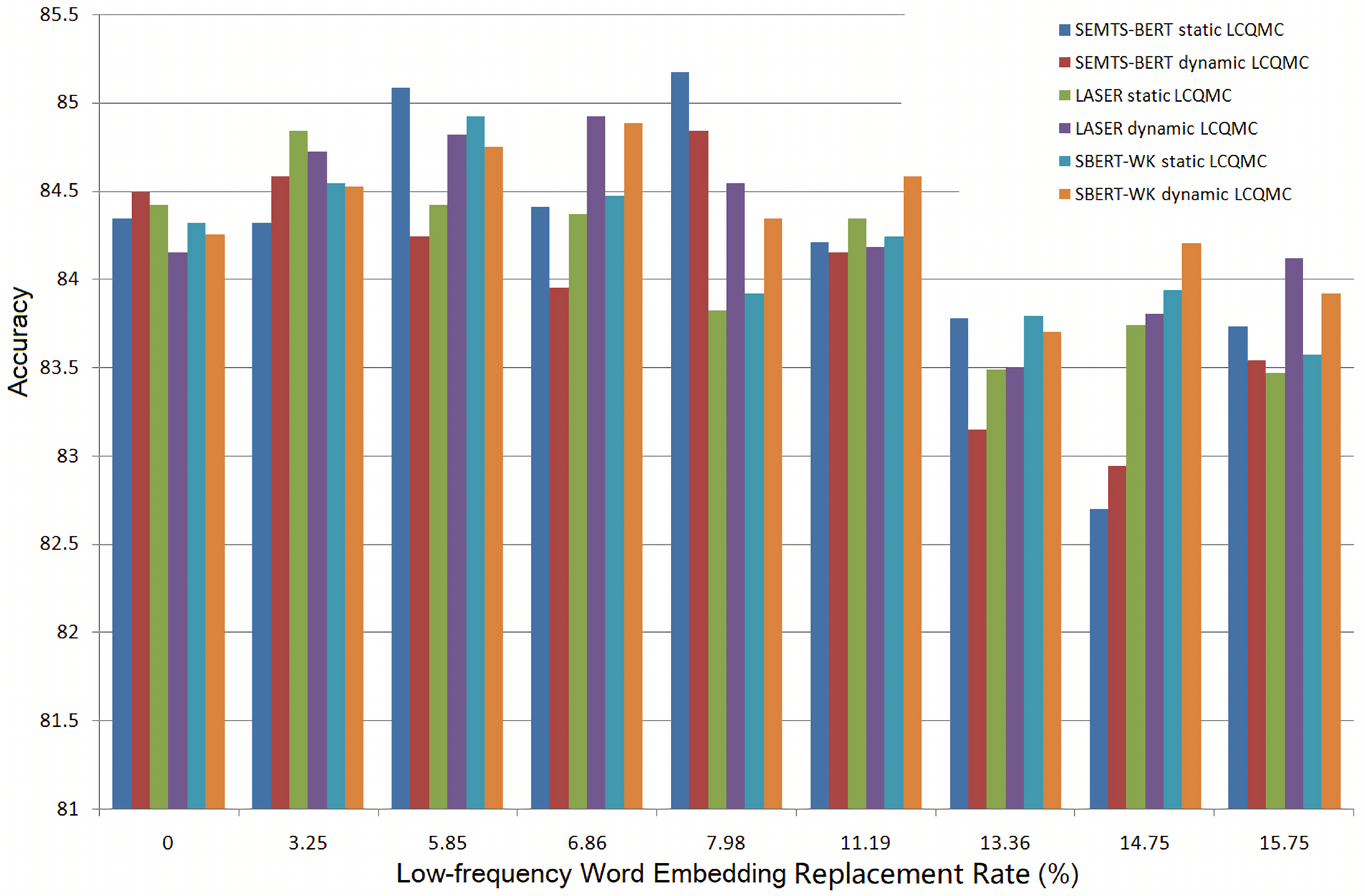
The situation in
Figure 12 is slightly different. On LCQMC, whether the word embeddings are dynamic or static, replacing low-frequency words’ embeddings can improve the performance of the word-based BiMPM. However, as the replacement rate increases, the performance of word-based BiMPM decreases significantly. When using LASER to estimate low-frequency words’ embeddings, the replacement can improve the accuracy of BiMPM at the rates of 3.25% (word embeddings are fixed) and 6.86% (word embedding are dynamic). We can draw the similar conclusion from the bars of SBERT-WK. When using SEMTS-BERT to estimate low-frequency words’ embeddings and the word embeddings are static, the replacement can effectively improve the accuracy of BiMPM from 84.34% to 85.08% and from 84.34% to 85.17% at the replacement rate of 5.85% and 7.98%. The best accuracy of BiMPM on LCQMC in [
38] is 83.34%, obtained by the character-based model. Our result is much better than the benchmark. When the word embeddings are dynamic, we can also draw a similar conclusion.
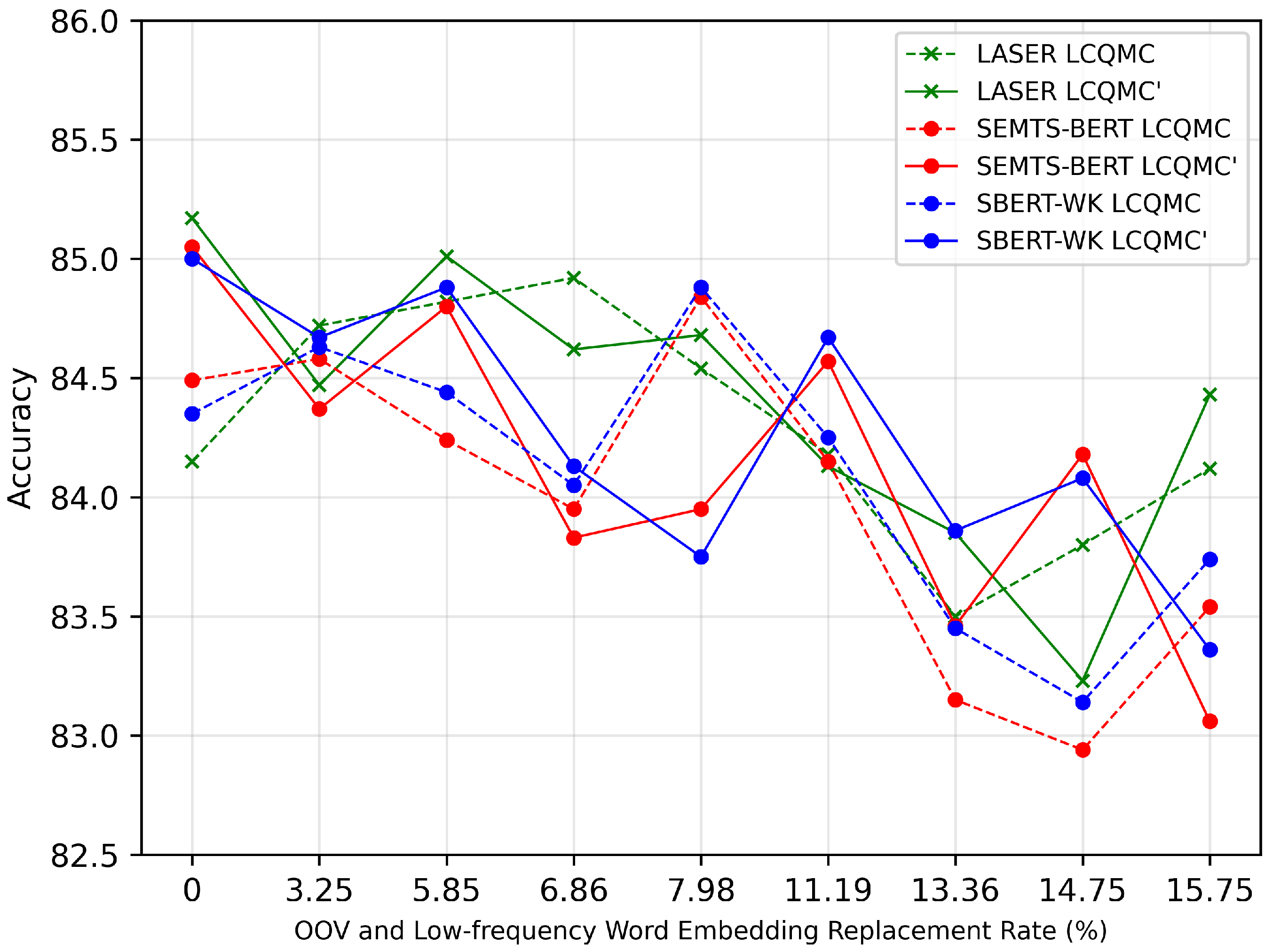
In addition, we obtain an interesting conclusion, which is shown in
Figure 13. When low-frequency words’ embeddings are not replaced, if the model has achieved good performance through the careful fine-tuning of hyper-parameters (the solid broken lines), then replacing low-frequency words’ embeddings can no longer improve the performance. On the contrary, if the performance of the model is relatively poor when no low-frequency words’ embeddings are replaced (the dashed broken lines), the replacement can improve the performance at some replacement rates. This conclusion can not only guide us to adjust hyper-parameters, but also enable us to obtain better performance by replacing the low-frequency words’ embeddings. This is because either we have obtained good performance or we will obtain better performance by replacing the embeddings of low-frequency words.
5.7.5. Analysis and Conclusion
Except for the condition that the word embeddings are static, replacing low-frequency words’ embeddings can hardly improve the performance on the smaller BQ dataset (take the benchmark as a reference). This may be caused by sparsity. On the larger LCQMC, the sparsity has been greatly alleviated. Regardless of whether the word embeddings are dynamic or static in the evaluation, replacing low-frequency words’ embeddings estimated by all sentence representation models can improve the performances of word-based BiMPM, and we achieve new benchmark on LCQMC.
However, only a suitable low-frequency word embedding replacement rate can improve the performance. The performance will be reduced when the replacement rate is too high. From our experimental results, the smaller the dataset, the more limited the performance improvement obtained by the replacement of low-frequency words’ embeddings. We think this is not only caused by sparsity, but also by the lack of coupling between the two different semantics spaces (the way that sentence representation models calculate word embeddings is different from the way that Word2Vec calculates word embeddings). In addition, if the model has achieved good performance when no low-frequency words’ embeddings are replaced, the replacement cannot improve the performance. On the contrary, if the performance is not good when no low-frequency words’ embeddings are replaced, the replacement will improve the performance.
In summary, we can draw two conclusions from the extrinsic evaluation. The first is that we can obtain higher-quality low-frequency word embeddings through our proposed method. When the dataset is large, replacing the original embeddings of low-frequency words in an appropriate proportion can improve the performance. The second is that SEMTS-BERT can represent the semantics of sentences well. This is because, on the BQ dataset, only SEMTS-BERT improves the performance of the word-based BiMPM, and on LCQMC, we achieve a new benchmark by using the embeddings estimated by SEMTS-BERT to replace the original embeddings of low-frequency words.
6. Discussion
The sparsity makes the semantics of words and phrases not fully learned, which in turn harms the performance of NLP tasks [
16,
17,
22,
25]. To reduce the sparsity, researchers have designed effective algorithms to split long words into short fragments. These algorithms include BPE and WordPiece [
1,
2,
20]. There is also a study pointing out that using character-level models in Chinese NLP tasks can achieve better performance [
16]. In this article, we use the dictionary to estimate the embeddings of low-frequency words. In extrinsic tasks, we obtain better performance by using word embeddings estimated by our proposed method to replace the original low-frequency words’ embeddings (estimated by Word2Vec). This shows that our method can provide higher-quality low-frequency word embedding. However, from the experimental results, we can see that too-high a replacement rate will harm the performance of tasks. In addition, performing such a replacement on a larger dataset will lead to higher performance improvement.
In this article, we design a new sentence representation model and expect to extract the semantics of explanatory notes more efficiently. Our sentence representation model achieves the best performance in many tasks in both the intrinsic and extrinsic experiments.
In summary, dealing with OOVs and low-frequency words is one of the challenges in NLP tasks. OOVs and low-frequency words are universal. Therefore, we think that it is very difficult to eliminate the OOV problem. Although the method proposed in this paper reduces the impact of the OOV problem on performance to a certain extent, there are still many problems worthy of further study. In the future, we will conduct in-depth research in the following aspects:
Use relationships between the rich nodes in knowledge bases to estimate the embedding of low-frequency words.
Construct more high-performance sentence representation models to extract semantics from sentences.
Since there are two different word embedding estimation methods, we will study measures to make two semantics spaces better coupled.
Use the correspondence between words in multilingual dictionaries to estimate the embeddings of low-resource language words.


